phic OSCAR-robot manipulator above an object which is arbitrary placed on a table. The ... Figure 1: OSCAR-robot manipulator. ..... Gram-Schmidt Neural Nets.
Predictive Robot Control with Neural Networks 1 2 G. Schram3 F.X. van der Linden B.J.A. Krose F.C.A. Groen Faculty of Mathematics and Computer Science, University of Amsterdam Kruislaan 403, NL-1098 SJ Amsterdam. Email:
Abstract
Neural controllers are able to position the hand-held camera of the (3DOF) anthropomorphic OSCAR-robot manipulator above an object which is arbitrary placed on a table. The desired camera-joint mapping is approximated by feedforward neural networks. However, if the object is moving, the manipulator lags behind because of the required time to preprocess the visual information and to move the manipulator. Through the use of time derivatives of the position of the object and of the manipulator, the controller can inherently predict the next position of the object. In this paper several `predictive' controllers are proposed, and successfully applied to track a moving object.
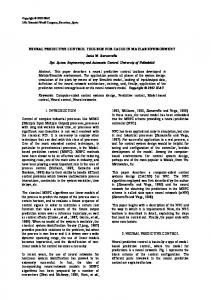
1 Introduction In [1] a real-time learning neural controller is described for the control of the (3DOF) anthropomorphic OSCAR-robot manipulator. An object, which is arbitrary placed on a table, is observed by a hand-held camera. Figure 1 shows a line drawing representation of the robot arm. θ3 θ4
θ2
θ5 θ6 camera
θ1
object
Figure 1: OSCAR-robot manipulator. In order to position the camera above the object, a feedforward network learns the camerajoint mapping. During operation, learning samples, one for each move, are obtained by the `input-adjustment-method' [2]. The learning samples are used to adapt the neural network. The task is restricted to 2D movements with the camera always looking down from a constant altitude. With this restriction just two joints angles, ~� = (�1 ; �2 ), have to be controlled. The joint angles �3 and �5 are expressed in terms of �1 and �2 , and the joint angles �4 and �6 are not used. Simulations show that the neural controller learns to position the camera above the object within 20 manipulator moves. However, if the object is moving on the table, the manipulator always lags behind because of the required time to preprocess the visual information and to move the manipulator. If time derivatives of the position of the object and of the manipulator are used, the controller may The project was partially sponsored by the Japanese RWC-project \Active Perception and Cognition". Submitted to Int. Conf. on Intelligent Autonomous Systems IAS-4, March 27-30 1995, Karlsruhe, Germany. 3 Currently working at the Delft University of Technology, Department of Electrical Engineering, Mekelweg 4, P.O.Box 5031, 2600 GA Delft, The Netherlands. 1 2
inherently predict the next object position. In this paper, a series of new `predictive' controllers is proposed and nally applied to the OSCAR-robot manipulator to track a moving object.
2 Predictive robot control The task of the controller is to minimize the position ~p = (x; y) of the object relative to the centre of the camera. The commands are de ned as joint displacements. Furthermore, we assume that the controller operates with a xed frequency: commands are generated equidistant in time. Suppose the controller generates a new command �~�k = (��1;k ; ��2;k ) at time step k. Then, for a moving object, a unique relationship exists between the desired joint displacements, and the position as well as its time derivatives of the object and of the manipulator: �~�k = F (p~k ; ~p_k ; ~pk ; ::; �~k ; ~�_k ; ~�k ; ::): Because of the structure of the OSCAR-robot manipulator, the position information of just one joint angle, �2 , is su�cient to describe the current state of the robot in the 2D case. This yields the following unique relationship: �~�k = F (p~k ; ~p_k ; ~pk ; ::; �2;k ; ~�_k ; ~�k ; ::): In fact, the time derivatives in the function F are used to predict inherently the next position of the object on the table. If the function F is approximated by neglecting the higher derivatives, we obtain several `predictive' controllers. Hereby, we expect that the more derivatives are used, the more accurate the approximation will be. If the manipulator is able to nish its move before a new command is given, the arm stands still each time a new observation is made. As a result, the angular velocities and accelerations of the robot arm are zero, and the time derivatives of the object position in the camera view correspond to those on the table. For this case, a series of three controllers with increasing complexity is directly found4: �~�k = �~�k = �~�k =
F0 (p ~k ; �2;k ); F1 (p ~k ; ~p_ ; �2;k );
k
F2 (p ~k ; ~p_ k ; ~pk ; �2;k ):
In practice however, it will be di�cult to measure explicitly the velocity and acceleration of the object from the noisy visual information. This problem can be circumvented by using previous positions of the object as inputs for the network. Together with the use of previous joint displacements, the controller should be able again to predict the next position of the object on the table. Also here we expect that the more previous positions and joint displacements are used, the more accurate the prediction of the object position and consequently the approximation of F will be. An extra advantage of this approach is that we can ignore the assumption of standing still each moment a new command is generated. Two controllers with increasing complexity are obtained: �~�k = F3 (p~k ; p~k 1 ; �2;k ; �~�k 1 ); �~�k = F4 (p~k ; p~k 1 ; p~k 2 ; �2;k ; �~�k 1 ; �~�k 2 ): Finally, we will investigate whether the task of predicting the next position of the object may be simpli ed by using the di�erence between two successive positions �p~k = ~pk p~k 1 as inputs 4
Note that F0 represents the original controller for positioning the camera above inert objects.
for the network. In fact, the di�erence serves as a primitive estimate of the velocity of the object in the image. Rewriting the controllers F3 and F4 with the slighty di�erent inputs yields: �~�k = �~�k =
F5 (p ~k ; �p ~k ; �2;k ; �~ �k F6 (p ~k ; �p ~k ; �p ~k
1 );
1; �2;k ; �~�k 1 ; �~�k 2):
3 Generation of learning samples The above mappings will be approximated by feed-forward neural networks. In order to build up a set of training samples for the networks, the `input-adjustment-method' [2] is used. The idea of the input-adjustment-method is to reconstruct those inputs that should have resulted in the desired performance. Suppose that one of the (not-perfect) networks F0 , F1 and F2 generates the output �~�k at time step k. After moving the robot, the object is observed again: ~pk+1. In the meantime, the camera is translated and rotated which can be expressed by a translation vector ~tk+1 and a rotation matrix Rk+1 of the second camera image with respect to the rst image. Figure 2 shows two successive camera images. image(k+1) Pk+1
) image(k
δ k+1 Pk
t k+1
Πk
Figure 2: Two successive images in order to reconstruct the inputs ~�k . The displacement of the object in the camera image ~�k+1 , expressed in the coordinates of the rst image, is obtained from the gure: ~ �k+1
=
h
�
Rk+1 p ~k+1
+ ~tk+1
i
p ~k :
The control task is to generate the joint displacements �~� which result in ~pk+1 = 0. If so, the displacement of the object in the image is expressed by ~�k+1 = ~tk+1 p~k . However, during learning this is not (yet) the case. What we can do, is reconstructing those inputs ~�k which had resulted in a perfect move: ~ �k
= ~tk+1 ~�h�k+1 � = ~tk+1 Rk+1 � ~ pk+1 + ~tk+1 = ~pk Rk+1 � ~pk+1:
pk ~
i
In other words, if a noving object was observed at position ~�, the joint displacement �~�k would have resulted in a ~pk+1 = 0. The reconstructed inputs together with the outputs �~�k yield a
learning sample. For the controllers F0 , F1 and F2 respectively, the input-output examples are written by: (~�k ; �2;k ) ! (�~�k ); (~�k ; ~p_k ; �2;k ) ! (�~�k ); (~�;k ; ~p_k ; ~pk ; �2;k ) ! (�~�k ): For the controller F3 , also the inputs p~k 1 have to be reconstructed. Using gure 3, the reconstructed inputs are obtained: ~�k 1 = ~pk 1 Rk � [Rk+1 � p~k+1 ]. image(k+1) Pk+1
) image(k
Pk
1)
ge(k
ima
Πk
Pk-1
Π k-1
Figure 3: Three successive images in order to reconstruct the inputs ~�k and ~�k 1 . A nearly similar reconstruction of the inputs ~pk 2 for controller F4 is not shown here. The reconstruction yields the following input-output examples for the controllers F3 and F4 , respectively: (~�k ; ~�k 1 ; �2;k ; �~�k 1) ! (�~�k ); (~�k ; ~�k 1 ; ~�k 2 ; �2;k ; �~�k 1 ; �~�k 2 ) ! (�~�k ): Finally, the inputs �p~k and �p~k 1 have to be reconstructed for the controllers F5 and F6 . Figure 3 shows that the reconstructed inputs �~�k are equal to ~�k ~�k 15 . Similarly, �~�k 1 = ~ �k 1 ~ �k 2 . The following input-output examples are obtained: (~�k ; �~�k ; �2;k ; �~�k 1 ) ! (�~�k ); (~�k ; �~�k ; �~�k 1; �2;k ; �~�k 1 ; �~�k 2) ! (�~�k ):
4 Simulations In order to compare the predictive controllers, a rst series of experiments was carried out with a simulation of the OSCAR-robot manipulator. For the simulations the test-environment `Simderella' is used [3]. Two object movements on the table serve as test cases; one follows the `daisy'-trajectory and one a random trajectory. The daisy is a `epicyclical' trajectory: two superposed circular movements. The random trajectory is generated as a small moving mass which is 5
Note that �~�k is not equal to �p~k .
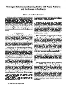
e�ected by a random force at each time step. Figure 4 shows the trajectories on the table. Both movements cover an area of about 40 by 40 cm. The base of the OSCAR-robot is situated at (0,0). y_table (cm)
y_table (cm)
20.00 20.00
10.00
10.00
0.00
0.00
-10.00
-10.00
-20.00 -20.00 50.00
55.00
60.00
65.00
70.00
75.00
x_table (cm) 80.00 85.00
x_table (cm) 50.00
55.00
60.00
65.00
70.00
75.00
80.00
85.00
Figure 4: Left: 200 points daisy trajectory, mean velocity is 3 cm/move. Right: 1000 points random trajectory, mean velocity is about 1 cm/move. The neural controllers consist of three (F0 ), ve (F1 ), seven (F2 , F3 , F5 ) or eleven inputs (F4 , F6 ), twenty hidden units with sigmoid activation functions, and two output units. The weights of the networks are adapted on-line by a conjugate gradient optimisation technique [4]. The algorithm is performed over the set of training examples which is build up using the inputadjustment-method. Simulations are done for 1000 moves of the manipulator. Each move lasts 0.5 seconds. The manipulator is in principle fast enough to follow the object. In table 1, the results of the simulations are given. The table shows the mean distance to the object in the image domain over the last 100 moves, averaged over three di�erent trials. controller F0 F1 F2 F3 F4 F5 F6
daisy random mean (cm) st.dev.(cm) mean (cm) st.dev.(cm) 5.0 1.3 1.08 0.05 0.79 0.07 0.24 0.03 0.16 0.07 0.20 0.02 1.09 0.12 0.47 0.01 0.27 0.03 0.52 0.09 1.08 0.05 0.29 0.01 0.26 0.05 0.59 0.08
Table 1: Results of simulations with daisy and random trajectory: mean distance to object over last 100 moves during learning, averaged over three trials. The predictive controllers follow the moving objects much better than the original controller F0 for inert objects. The results of F1 and F2 are of course the best, although these controllers are not practical because of the assumption of perfect velocity and acceleration measurements. In general, we see that the more derivatives or the more previous positions are used, the better the tracking performance. This agrees with our expectations of section 2. The bound of this
statement is immediately illustrated by the exceptions F4 and F6 for the random trajectory. Since the acceleration of the object is randomly generated and the mass of the object is rather small, the correlation between four successive positions (between ~pk 2 and ~pk+1) is neglectible. Therefore the inputs ~pk 2 did not contribute to a more accurate prediction of the next object position. The nal results of F5 relative to F3 , and F6 relative to F4 hardly di�er for the daisy trajectory. This is not surprising since the available information is not changed. Remarkable is the outstanding performance of F5 relative to F3 in case of the random trajectory. Obviously, the primitive estimate of the velocity has simpli ed the learning task. This is con rmed by the learning performance of the controllers. The distance to the object converged a factor 2 to 3 faster for F5 relative to F3 and for F6 relative to F4 . Figure 5 shows the learning curves of F3 up to F6 of one trial for the daisy test case. dist (cm)
dist (cm)
10.00
10.00
controller F3
8.00
controller F4
8.00
6.00
6.00
4.00
4.00
2.00
2.00
0.00
0.00 0.00
0.20
0.40
0.60
0.80
10^3 moves 1.00
dist (cm)
0.00
0.20
0.40
0.60
0.80
10^3 moves 1.00
dist (cm)
10.00
10.00
controller F5 8.00
8.00
6.00
6.00
4.00
4.00
2.00
2.00
0.00
controller F6
0.00 0.00
0.20
0.40
0.60
0.80
10^3 moves 1.00
0.00
0.20
0.40
0.60
0.80
10^3 moves 1.00
Figure 5: Results of simulation with daisy trajectory: faster convergence of distance to object for F5 relative to F3 and for F6 relative to F4 . The fast convergence can be explained by the decorrelation of the inputs of the network. In general, decorrelating the inputs results in faster convergence for linear combiners [5]. This can be understood by noting that, if the inputs are strongly correlated, the combiner has to linearly combine a lot of redundant information, and will be slow in learning the statistics of the input data. Since the units in the rst layer of our network are linear combiners followed by a sigmoid function, this theory holds also for our ndings [6]. A measure of correlation is the spread of the eigenvalues �max =�min of the correlation matrix
= E [~u~uT ] of the input vector ~u. The smallerPthe spread, the faster the network adapts. The correlation matrix can be estimated by R^ = patterns ~u~uT . For the controllers F3 and F5 the correlation matrix is estimated over 500 moves of which the spread of the eigenvalues is determined. The results, averaged over three trials, show that the spread is indeed decreased by approximately a factor two (table 2). R
controller F3 F5
daisy random mean st.dev. mean st.dev. 368.5 74.8 54.3 6.5 205.4 29.5 27.9 7.4
Table 2: Spread of eigenvalues �max =�min for daisy and random trajectory, averaged over three trials.
5 Experiments with OSCAR-robot Finally, in order to illustrate the bene ts of the predictive controllers, two experiments are carried out with the real OSCAR-robot manipulator. The task of the manipulator is to track a moving cart on the table. The control cycle is xed at 1 s. The cart arbitrary moves with a velocity of approximately 5 cm/s within an area of about 45 by 45 cm. The manipulator is in principle fast enough to follow the cart. For the original controller F0 and the predictive controller F5 , the distance from the object to the centre of the camera image during learning is plotted in gure 6. The distance is expressed in camera units; 3 camera units correspond to approximately 2 cm on the table. For F0 and F5 the mean distance to the object is, averaged over the last 100 moves, 7.1 and 1.2 camera units, respectively, corresponding to 4.8 and 0.8 cm. It is clear that the new approach improved the tracking performance considerably. dist (camera units)
dist (camera units)
20.00
20.00
16.00
16.00
12.00
12.00
8.00
8.00
4.00
4.00
0.00
0.00 moves 0.00
100.00
200.00
300.00
0.00
100.00
200.00
moves
300.00
Figure 6: Results of experiments with OSCAR-robot: distance to object for original (left) and predictive (right) controller. 3 camera units correspond to � 2 cm on the table. In gure 7 the position of the object in the camera image is plotted. The gure shows that the original controller lags behind: the cart is moving with a velocity of about 5 cm/s � 7.5 camera units/move. In constrast, the predictive controller is able to anticipate the movement of the object.
y (camera units)
y (camera units) 10.00
10.00
6.00
6.00
2.00
2.00
-2.00
-2.00
-6.00
-6.00
-10.00
-10.00
-10.00
-5.00
0.00
5.00
x (camera units) 10.00
-10.00
-5.00
0.00
5.00
x (camera units) 10.00
Figure 7: Results of experiments with OSCAR-robot: camera view of object for original (left) and predictive (right) controller. 3 camera units correspond to � 2 cm on the table.
6 Conclusions Through the use of time derivatives of the position of the object and of manipulator, neural controllers are obtained which can inherently predict the next position of the object. Generally, the more time derivatives are used, the more accurate the neural controller will be, as long as the object movement can be predicted in principle. Instead of taking time derivatives, also previous positions of the object and manipulator yield predictive controllers. If the correlation between these inputs can be decreased by using the di�erences between successive positions, faster convergence is obtained for the network. The new approach resulted in a real-time learning `predictive' controller for the OSCAR-robot manipulator. The manipulator learned to track a moving object succesfully.
References [1] Smagt PP van der, Krose BJA (1991). A real-time learning neural robot controller. In Proc. ICANN-91. Eds Kohonen T, Makisara K, Simula O, Kangas J. Espoo, Finland. pp 351-356. [2] Krose BJA, van der Korst MJ, Groen FCA (1990). Learning strategies for a vision based neural controller for a robot arm. In: IEEE international workshop on intelligent motor control. Eds Kaynak O. Istanbul. pp 199-203. [3] Smagt PP van der (1994). Simderella: a robot simulator for neuro-controller design. Neurocomputing, vol 6, no 2. [4] Smagt PP van der (1994). Minimisation methods for training feed-forward neural networks. Neural Networks, vol 7, no 1. pp 1-11. [5] Widrow B, Stearns SD (1985), Adaptive Signal Processing. Prentice-Hall Inc, Englewood Cli�s. [6] Orfanidis SJ (1990). Gram-Schmidt Neural Nets. Neural Computation, vol 2, pp 116-126.