Preferential Flow in the Field Soils - scipress

Original Paper __________________________________________________________ Forma, 17, 31–53, 2002

Preferential Flow in the Field Soils Susumu O GAWA1*, Philippe BAVEYE 2, Jean-Yves P ARLANGE2 and Tammo STEENHUIS2 1

Graduate School of Environmental Systems, Faculty of Geo-Environmental Science, Rissho University, 1700 Magechi, Kumagaya, Saitama 360-0194, Japan 2 Department of Agricultural and Biological Engineering, Cornell University, Ithaca, NY 14853, U.S.A. *E-mail address: [email protected]

(Received April 8, 2002; Accepted August 20, 2002)

Keywords: Fractal, Image Processing, Dyed Images, Infiltration Abstract.

Preferential flow has been increasingly recognized as a process of great practical significance for the transport of water and contamination in field soils. Recently, fractal has been applied to characterize the geometry of stain patterns of soil profiles. The field experiment involved loamy and sandy soils. The sequence of images of horizontal cross-sections of stain patterns in the two soils suggest that fingering occurred in the loamy soil, not in the sandy soil. Yet, the surface fractal dimensions of the stain patterns are very similar in both cases. This similarity suggests that these dimensions provide information not so much on the geometry of the stain patterns but more directly on the fractal properties of the pore network in the soil. This viewpoint is confirmed partially by the evidence of a good correlation between the surface fractal dimension and the exponent of a Van Genuchten expression applied to the particle size distribution of the soil.

1. Introduction Preferential flow involves the transport of water and solutes via preferred pathways through a porous medium (HELLING and G ISH, 1991; S TEENHUIS et al., 1995). During preferential flow, local wetting fronts may propagate to considerable depths in a soil profile, essentially bypassing the matrix pore space (BEVEN, 1991). Although the term preferential flow does not imply any particular mechanism, it usually refers to one (or more) of three physically distinct processes: macropore flow, fingering (unstable flow), and funneled flow. Macropore flow involves transport through noncapillary cracks or channels within a profile, reflecting soil structure, root decay, or the presence of wormholes and ant or termite tunnels. A well-structured soil, for example, has two more or less interconnected flow regions for liquids applied at the surface: (1) through the cracks between blocks (interpedal transport), and (2) through the finer pore sequences inside the blocks (intrapedal, or matrix transport). Fingering, which occurs as a result of wetting front instability, may cause water and solutes to move in columnar structures through the vadose zone at velocities approaching saturated pore velocity (GLASS et al., 1988). Fingering may occur for a number of reasons, including changes in hydraulic conductivity with depth and compression of air ahead of the 31

32

S. O GAWA et al.

wetting front (HELLING and GISH, 1991). Funneled flow, finally, occurs when sloping geological layers cause pore water to move laterally, accumulating in a low region. If the underlying region is coarser-textured than the material above, fingering may develop. In a number of studies, the occurrence of preferential flow has been deduced indirectly from the inability of traditional transport equations (e.g., the Richards equation) to predict the outcome of breakthrough experiments in undisturbed soil columns, lysimeters or tiledrained field plots (e.g., RADULOVICH et al., 1992; MC COY et al., 1994). Various experimental techniques have been used to get insight into the processes that control preferential flow and in particular to identify the soil characteristics (e.g., macropores, cracks, etc.) that are responsible for preferential flow. Examples of such experimental techniques include X-ray computed tomography (GREVERS et al., 1989; PEYTON et al., 1994) or micromorphological analysis of soil thin sections (GREVERS et al., 1989; AGUILAR et al., 1990). Most of the studies on preferential flow, however, have relied on the use of dyes to visualize the preferential flow of water and solutes in soils, in laboratory experiments or under field conditions (e.g., BOUMA and DEKKER, 1978; HATANO et al., 1983; RADULOVICH and S OLLINS, 1987; GHODRATI and J URY, 1990; F LURY et al., 1994; F LURY and FLÜHLER , 1995; NATSCH et al., 1996). Color or black-and-white pictures of dye-stained soil profiles may be analyzed to provide the percentage of stained areas in vertical or horizontal cuts in the soil (e.g., NATSCH et al., 1996). As useful as the information contained in these percentages may be to predict the extent and the kinetics of preferential flow in soils, one would undoubtedly want a more detailed description of the geometry of stain patterns and some way to relate this geometry to know morphological features of the soils. In this respect, the close similarity that is often apparent between these stain patterns and the very intricate details exhibited by fractals has encouraged a number of researchers to apply the concepts of fractal geometry to characterize preferential flow pathways. This approach was pioneered by H ATANO et al. (1992) and HATANO and BOOLTINK (1992). These authors reported that the geometry of stain patterns in two-dimensional images of soil profiles may be characterized very accurately with two numbers; a fractal dimension associated with the perimeter of the stain patterns and another fractal dimension, relative to their surface area. The first fractal dimension varied little among-, or with depth within, the five soils tested by HATANO et al. (1992). However, the second fractal dimension, known as a “mass fractal dimension” in the literature on fractals, varied appreciably both among soils and with depth for a given soil, with a total range extending from 0.59 to 2.0. One way to consider these results is that the mass fractal dimension, being apparently the most sensitive descriptor of the geometry of preferential flow pathways, contains more information on the processes that influence these pathways, than the comparatively more constant “perimeter” or “surface” fractal dimension. From this viewpoint, the mass fractal dimension would serve as a good basis for comparison among soils. The fact that, in H ATANO et al.’s (1992) experiments, the mass fractal dimension assumes values as low as 0.59, when intuitively one would expect it to be equal to 2 in twodimensional cross sections, suggests that something is astray in the evaluation of this dimension and that a detailed examination of the methodology in use is warranted. The determination of fractal dimensions of objects, based on the analysis of digitized images, unavoidably involves a number of subjective choices. Examples are the type of camera

Preferential Flow in the Field Soils

33

used to take pictures, the sensitivity of the film, the angle and field of view, the resolution of the scanner used to digitize the image, the choice of a threshold to transform the images from grayscale to binary (e.g., dye and non-dye), and finally the choice of a fractal dimension from among the infinitely many dimensions available. Each and every one of these subjective choices might cause the resulting fractal dimension to wander outside the range of physically plausible values and may lead different observers to obtain very different estimates of the fractal dimension of a given stain pattern in a soil. This situation is in no way unique to the application of fractal geometry to preferential flow processes, as stressed recently by DUBUC and DUBUC (1996): “...different methods as well as different scale ranges and resolutions can lead to estimate of dimension that are drastically different. Estimates of fractal dimension will never be valuable until one fully understands the importance of the various error factors involved in the estimation process.” In particular, whenever fractal dimensions are evaluated on the basis of digitized images (e.g., BARTOLI et al., 1991; CRAWFORD et al., 1993a, b; CHIANG et al., 1994; M OORE and DONALDSON , 1995; A NDERSON et al., 1996), subjective, operator-dependent, choices have to be made. At present, the effect of these choices on the evaluation of fractal dimensions is not known, nor even acknowledged until very recently. Furthermore, the theoretical framework necessary to interpret the influence of some of these choices, particularly the effect of image resolution, is lacking. A field experiment was carried out to determine how the surface fractal dimension of a stain pattern varies with depth, in the presence and absence of preferential flow. A secondary motivation of this experiment was to gain insight into the physical meaning of the fractal dimensions of stain patterns. 2. Materials and Method 2.1. Field site The field site is located in the old Cornell University orchard and in a neighbouring pasture, in Ithaca (New York). Soils in this orchard are moderately well-drained, were formed on a lacustrine deposit, and have been classified alternatively as a fine, illitic, mesic, Glossaquic Hapludalf (V ECCHIO et al., 1984) or as a mixed, mesic Udic Hapludalf (MERWIN and STILES, 1994). The orchard was originally planted in 1927, but the trees were removed in 1977–78. Between 1979 and 1983, a variety of test crops, including tobacco, sunflower and vegetables were grown on the plot. In 1985, the site was deeply plowed with 12 T/ha of dolomite lime, and ryegrass and red fescue were planted (MERWIN and S TILES, 1994). In April 1986, dwarf apple trees were planted 3 m apart in rows spaced 6 m. Sod grass ground cover has since been maintained between the tree rows and has been regularly mowed to a height of 6–10 cm. Most soils in the pasture are Arkport fine sandy loam. The Arkport series consists of well drained sandy soils (CLINE and BLOOM, 1965). The topography of this unit consists of small knolls and slight depressions. The upper part of the soil to a depth ranging from 50 to 90 cm has been leached and has been weathered slightly, leaving a thin yellowish

34

S. O GAWA et al.

brown coating of iron and organic matter on the sand grains. It has the moderate available moisture capacity typical of fine sandy loam materials. Below this layer and extending to a depth ranging from 1.2 to 2.4 m is a zone within which small amounts of silicate clay have been segregated in dark brown bands 3 to 25 mm thick and 10 to 44 cm apart. These coherent bands retard downward movement of water and contribute to higher water supplying capacity than typical of the dominant loamy fine sand or fine sand texture of the zone. Beneath the banded zone are layers of sand of varying fineness, locally with thin lenses of silt. 2.2. Dye experiment The pictures for this paper were obtained on July 30, August 11, 14, and 19, 1997. Twenty liters of a 1% solution (10 g/l) of blue food coloring (F&DC Blue#1) and calcium chloride were poured into a metal cylinder with 30 cm in diameter. In the case of Orchard 1, ten liters of the same solution was used. Fifteen minutes to one hour later, a trench was dug by 1.8 m in depth, tangential to the outer surface of the metal ring. Initial digging was done with a backhoe, followed by carefully removing soil with shovels in order to obtain as horizontally as possible a soil profile. Color pictures were taken of the exposed soil facies with a camera fixed to the steel stand with 2 m in height. Then a 2 cm-thick slice of soil was further excavated on the surface of soils. This same procedure was repeated 20 to 60 times, at about 2 cm intervals, to obtain evidence of dye preferential transport at various points underneath the metal ring. 2.3. Image manipulation Twenty to sixty different pictures of a single soil facies were used for this paper. The slides were scanned and resulting (2048 × 3072) digitized images were stored in RGB (redgreen-blue) color-coding format on a Kodak CD-ROM. The software Adobe PhotoshopTM was used to manipulate and analyze soil images. To ensure that all digitized images would receive identical treatments, precisely the same field of view was “cropped” (i.e., delineated and cut) in each case. In addition, to maximize the contrast between stained and background soil material, the storage format of the cropped images was changed from RGB to CYMK (cyan-yellow-magenta-black), and the cyan channel was retained for further analysis. This channel corresponds very closely with the color of the dye used in the field experiment, a feature that makes the stain patterns much more sharply contrasted than for any of the other channels available in Adobe PhotoshopTM. For the remainder of the work, the cyan channel of each image was converted to a grayscale image. However, in this case, the Lab color system was used instead of CYMK to obtain grayscale images. The Lab color system is similar to hue mode and is defined relative to two axes, a and b, and intensity. While the axis a covers green to pink, the axis b covers blue to yellow. These axes have two sharp Gaussian peaks corresponding to blue dyed and soil parts. 2.4. Thresholding algorithms To threshold or “segment” a digitized image, one could in principle proceed by trial and error until one achieves a thresholding that appears reasonable, i.e., coincides with


35

some a priori idea one may have about the two categories of pixels one attempts to separate. Unfortunately, this procedure is very subjective and may lead to biases when one is trying to compare images, or in the analysis of time sequences of images of a given object (e.g., under evolving lighting conditions). To palliate these difficulties, numerous automatic, non-subjective thresholding algorithms have been developed (e.g., G LASBEY and HORGAN , 1995). Two of the most commonly used were adopted in the research described in the present article. Both are iterative. The Intermeans algorithm is initiated with a starting “guess” for the threshold. Then the mean pixel value of the set of pixels with grayscale level greater than the initial threshold is calculated, and likewise for the set of pixels with grayscale level less than or equal to the initial threshold. The average of these two means is calculated, and truncated to an integer, to give the next “guess” for the threshold. This process is continued, iteratively, until it converges, i.e., until there is no change in the threshold from one iteration to the next. In the Minimum-Error algorithm, the histogram is visualized as consisting of two (usually overlapping) Gaussian distributions. As with the Intermeans algorithm, a starting “guess” for the threshold is made. The fraction of the pixels in each of the two sets of pixels defined by this threshold is calculated, as are the mean and variance of each of the sets. Then, in effect, a composite histogram is formulated, which is a weighted sum of two Gaussian distributions, each with mean and variance as just calculated, and weighted by the calculated fraction. The (not necessarily integer) grayscale level at which these two Gaussian distributions are equal is calculated (involving solution of a quadratic equation). This grayscale level, truncated to an integer, gives the next “guess” for the threshold. Again, the process is continued, iteratively, until it converges. Both thresholding algorithms suffer from the fact that the choice of the starting guess used to initiate the iterative calculation influences the convergence to a final threshold value. The resulting indeterminacy was avoided by using an objective approach developed by BOAST and BAVEYE (1997). 2.5. Removal of islands and lakes After thresholding the images of soil profiles with one of the algorithms described above, the resulting geometrical structure is generally very disconnected; besides two or three large “continents” that extend downward from the soil surface, there is a myriad of “islands” of various sizes and shapes. Some of these islands may in fact be peninsulas, artificially separated from the continents by the coarse-graining associated with the generation of images at a specified resolution. Some of the islands, however, may be truly disconnected from the continents, and may be manifestations of 3-dimensional flow, not strictly in the plane of the images. For the purpose of describing one-dimensional preferential flow in field soils, one may want to restrict application of fractal geometry to the part of a stain pattern that is connected to the inlet surface. This can be achieved with Adobe Photoshop by selecting the continents with the magic wand tool, inverting the selection (i.e., selecting everything but the continents), and making the latter selection uniformly white by adjusting its contrast and brightness. This procedure effectively eliminates islands.

36

S. O GAWA et al.

In a similar manner, even though a physical justification is less obvious in this case, it is possible to remove the “lakes”, or patches of unstained soil within the continents. However, the lakes and islands in the images used for this paper were not mainly removed. 2.6. Calculation of fractal dimensions The box-counting, information and correlation dimensions were calculated using the C++ code “fd3” written by John Saraille and Peter Di Falco (California State University at Stanislas). This code, widely available on the Internet at, e.g., http://hpux.ced.tudelft.nl/ hpux/Physics/fd3-0.3.html, is based on an algorithm originally proposed by LIEBOVITCH and TOTH (1989). As do virtually all other algorithms that are meant to evaluate fractal dimensions of geometrical structures in a plane, fd3 only considers the centroids of the various pixels constituting the images of these structures. The side of the smallest square that fully covers the given set of points is successively halved 32 times, yielding box coverages with progressively smaller boxes. The two largest box sizes are considered too coarse and are therefore not taken into account in the calculation of the box-counting, information, and correlation dimensions. Similarly, at the low end of boxes is equal to the total number of points (=number of pixels in the image), are ignored. The box-counting dimensions of several of the stain patterns were also calculated using a Pascal code written especially for the present work. 2.7. Soil tests 2.7.1 Water content and bulk density Water content is measured via the gravimetric method, which involves weighing the wet sample, removing the water by oven drying, and reweighing the sample to determine the amount of water removed. Water content is often obtained by dividing the difference between wet and dry masses by the volume of the sample cylinder to give the ratio of the volume of water to the volume of the whole soil (KLUTE, 1986). Bulk density is determined on the same samples by dividing the oven-dry mass by the volume. Sampling cylinder size is 54 mm in diameter and normally 30 mm in height, except when finer depth-resolution was necessary, in which case cylinders with a 10 mm height were used. An oven is controlling the temperature of 100°C. The oven time is 24 hours for each sample. 2.7.2 Porosity Calculating porosity from density measurements simply involves converting data from densities to volume. That is, from dry bulk density D b and the particle density, porosity is calculated with the next relationship (KLUTE, 1986).

(

)

φ = 1 − Db / ρ p .

(1)

2.7.3 Conductivity Hydraulic conductivity of saturated samples is measured by constant head method with steady upward flow (KLUTE, 1986). Sampling cylinder size is 76 mm in diameter and 76 mm in height. The steady upward flow into soils is controlled at a constant flow rate by a chemical pump. The samples are saturated with water before the test.


37

2.7.4 Particle size distribution The samples are dried in an oven for 24 hours at 100°C and are reduced to a powder state in a mortar. For each sample, the various size fractions are collected on screens of successively smaller size, and the amount in each fraction is determined by weighing. To separate and classify fine particles (less than 0.05 mm), the sedimentation method is used, based on measuring the relative settling velocity of particles of various sizes from the aqueous suspension according to Stoke’s law (KLUTE, 1986). 2.7.5 Soil moisture characteristic curves Soil moisture characteristic curves are obtained with a small Hele-Shaw-type chamber (BAUTERS et al., 1997). The chamber size is 57 cm in height, 45 cm in length, and 6 mm in width. The chamber is filled with the soil, at a bulk density realistically close to the field bulk density. A dry state is obtained from an initially saturated state via upward adsorption in about one week. After that, water content at each height is measured and the drying and wetting moisture characteristic curves are established. 2.7.6 Chloride test The concentration of calcium chloride in soils is measured with the silver chloride method. Sampling cylinder size is 54 mm in diameter and 10 mm in height. The sample is dried in an oven for 24 hours, weighed, and dissolved into deionized water. The solution of calcium chloride is tested with the silver chloride method. In this case, digital chloridometer (Buchler Instruments) is used for the identification of the concentration of calcium chloride. Finally, the concentration of calcium chloride is expressed as the ratio of its mass to the mass of the dry soil (in mg/g). 3. Theory Many soil properties have been described with fractal geometry. First, water retention curves for the BROOKS and COREY (1964) or CAMPBELL (1974) power function were parameterized with fractal dimension (TYLER and WHEATCRAFT, 1990).

ψ = ψ e (θ / θ s )

−1 / ( 3 − D )

(2 )

where ψ and ψe are water retention and air entry pressure, and θ and θs are water content and saturated water content. The fractal dimension D relates to the original exponent as

(3)

D = 3−λ

where λ is the exponent (BROOKS and COREY, 1964). In the same way, soil particle-size distributions were also described using fractal concepts (TURCOTTE, 1986; TYLER and WHEATCRAFT, 1992).

M ( r < d ) / MT = ( d / d L )

3− D

( 4)

where M and MT are the mass of particles with r < d and the total mass, respectively, and

38

S. O GAWA et al.

d, r, and dL are grain size, a specific measuring scale, and a constant, respectively. The former fractal dimension is less than the latter (TYLER and WHEATCRAFT, 1992). Actual soil particle-size distributions obey to Van Genuchten model (VAN G ENUCHTEN, 1980) very well (HAVERKAMP and PARLANGE, 1986). F=

1   dg  n  1 +      d  

m

(5)

where F is the cumulative particle-size distribution function, and dg, m, and n are constants. The constants m and n have the next relationship. m = 1 – 1/n

(6)

n = λ + 1.

(7)

and

Therefore, from the Van Genuchten model, a fractal dimension may be obtained. On the other hand, from the water retention curves some soil properties were obtained theoretically (CAMPBELL, 1985). Among them hydraulic conductivity is the most important.

k = ks (θ / θ s )

2b + 2

(8)

and

ks =

σ w2 θ s2 2 ρνψ e2 (2 b + 1)(2 b + 2)

( 9)

where ks is saturated conductivity, σ w the surface tension of water, ρ water density, ν kinematic viscosity, and b an exponent of water retention curves. The exponent b relates with the exponent λ and fractal dimension. b = 1 / λ = 1 / (3 − D).

(10)

Thus, from Eqs. (8), (9), and (10), the next relationship are obtained. 8−2 D

k = ks (θ / θ s ) 3 − D and

(11)


ks =

σ w2 θ s2 (3 − D) 2 ρνψ e2 (5 − D)( 4 − D)

39

(12)

the exponent b denotes the slope of the pore size distribution. Empirically the following equations were obtained (CAMPBELL, 1985).

ψ es = −0.5d −1.2

(13)

b = d −1.2 + 0.2σ

(14)

and

where ψes is the air entry potential for standard dry soils in J/kg, d is the geometric mean in mm, and σ is the geometric standard deviation of soil particle size (dimensionless). Therefore, some soil properties are described with the use of fractal dimensions. Fractal dimension is also calculated from soil particle-size distributions and water retention curves. The images of preferential flow in soils might reflect one or more soil properties that are described with fractal dimensions.

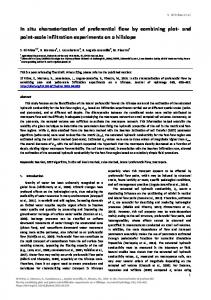
Fig. 1. Dyed images of cross sections in Orchard 1 (a) at depth 2.8 cm, (b) at 11.3 cm, (c) at 19.2 cm, and (d) at 28.3 cm.

40

S. O GAWA et al.

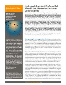
4. Results 4.1. Preferential flow images and their fractal dimension Four cases showed some characteristic images, islands, lakes, networks and dispersion (Figs. 1, 2, 3, and 4). Islands are black small areas in Figs. 1, 2, and 4, and show fingers in preferential flow. Lakes are white small areas in Figs. 3 and 4 and show spotted clay soils. Networks are black connected pathways in Fig. 2 and show the body of preferential flow. Dispersion is black traces in Fig. 2 and show front edge of flow. Table 1 shows the fractal dimension of these patterns. One case in Fig. 2 (Orchard 2) showed typical preferential patterns. Fractal dimension changes from 1.2 to 1.48. Fractal dimension is larger than 1.3 for islands and lakes, and larger than 1.4 for networks and dispersion. Preferential flow is the phenomenon of bifurcation of flow pathways. Fractal dimensions increase corresponding to this bifurcation, preferential flow. Preferential flow occurred in Fig. 2 because the hydraulic conductivity might increase with depth. 4.2. Soil tests Some soil tests were carried out for these cases (Table 2). Orchards 1 and 2 are sandy clay including wormholes and cracks. Pastures 1 and 2 are sandy loam and sandy clay loam (at the surface). Each soil texture is almost uniform except its surface. While Pasture 1 and Orchard 1 are in dry state, Pasture 2 and Orchard 2 are in wet state.

Fig. 2. Dyed images of cross sections in Orchard 2 (a) at depth 4.2 cm, (b) at 27.1 cm, (c) at 51.5 cm, and (d) at 81.1 cm.


41

Fig. 3. Dyed images of cross sections in Pasture 1 (a) at depth 5.1 cm, (b) at 16.3 cm, (c) at 32.7 cm, and (d) at 44.2 cm.

Fig. 4. Dyed images of cross sections in Pasture 2 (a) at depth 2.2 cm, (b) at 26.1 cm, (c) at 42.6 cm, and (d) at 62.9 cm.

42

S. O GAWA et al.

Table 1. Fractal dimension for cross section images in preferential flow. D represents fractal dimension, or capacity dimension. The figures show the range of the fractal dimension.

Location Fractal dimension Image patterns

Orchard 1

Orchard 2

Pasture 1

Pasture 2

1.2 ≤ D ≤ 1.5

1.2 ≤ D ≤ 1.5

1.2 ≤ D ≤ 1.5

1.2 ≤ D ≤ 1.5

Islands (D ≥ 1.3) Networks (D ≥ 1.4) Dispersion (D ≥ 1.4)

Lakes(D ≥ 1.3)

Islands (D ≥ 1.3)

Islands (D ≥ 1.3) Lakes(D ≥ 1.3)

Fig. 5. Soil size distribution for Orchard 2. The fitting curves are the van Genuchten type. Each sample depth is (o1) 5.4 cm, (o2) 5.4 cm, (o3) 7.2 cm, (o4) 16.1 cm, (o5) 26.8 cm, (o6) 37.5 cm, (o7) 48.2 cm, (o8) 49.2 cm, (o10) 84.1 cm, and (o11) 114.3 cm, respectively.

Table 2 shows the averages for these results. The soil at Orchard 2 has low infiltration rate, high porosity, and a low λ value. Figures 5 and 6 show soil particle-size distributions for Orchard 2 and Pasture 2. Most points fit Van Genuchten curves. Figure 7 shows soil texture; soils in Orchard are sandy clay and soils in Pasture are sandy loam. Both soil textures look continuous with depth. The saturated conductivity increases with depth in any cases as shown in Fig. 8. Figures 9 and 10 show water content and porosity change with depth. In all the cases, unsaturated flow occurred and degree of saturation was around 50%. The initial water content and the final water content were very near. The images of cross sections in wet state are broader than in dry state. Figure 11 shows calcium chloride and 7.5


43

Table 2. Field soil test results. Infiltration rates show the time-averages of the infiltration rates. The rest values are the average of the total soil test results each case. The value λ is an exponent of the modified Van Genuchten curve for soil particle-size distribution. Chloride means the concentration of calcium chloride in dry state soils (in mg/g). Location Infiltration rate (cm/s) Initial water content Porosity Mean particle size (mm) Conductivity (cm/s) λ Chloride (mg/g)

Orchard 1 0.0243 0.0736 0.468 0.0368 0.152 0.352 —

Orchard 2

Pasture 1

Pasture 2

0.00475 0.301 0.501 0.0452 0.0259 0.354 0.705

0.0187 0.0537 0.441 0.240 0.0442 1.84 0.634

0.0104 0.141 0.442 0.240 0.0103 1.21 0.514

Fig. 6. Soil size distribution for Pasture 2. The fitting curves are the van Genuchten type. Each sample depth is (p1) 6.5 cm, (p2) 19.5 cm, (p3) 32.5 cm, (p4) 44.0 cm, (p5) 54.0 cm, (p6) 63.8 cm, (p7) 71.3 cm, and (p8) 78.8 cm, respectively.

mg/g is saturated state in soils, the result shows that solution decreases exponentially. Tables 3 and 4 show soil test results in the cases of Orchard 2 and Pasture 2. Mean particle sizes in both cases are quite different. The mean particle size in Orchard 2 increases with depth while that in Pasture 2 keeps almost constant. This increase of the mean particle size in Orchard 2 makes the increase of hydraulic conductivity, which may cause preferential flow.

44

S. O GAWA et al.

Fig. 7. Soil texture. Pasture sample depths are at (1) 5.1 cm, (2) 6.5 cm, (3) 19.5 cm, (4) 32.5 cm, (5) 44.0 cm, (6) 54.0 cm, (7) 54.2 cm, (8) 63.8 cm, (9) 71.3 cm, (10) 78.8 cm, respectively. Orchard sample depths are at (1) 5.4 cm, (2) 7.2 cm, (3) 16.1 cm, (4) 26.8 cm, (5) 29.7 cm, (6) 37.5 cm, (7) 48.2 cm, (8) 49.2 cm, (9) 59.2 cm, (10) 84.2 cm, (11) 114.3 cm, respectively.

Fig. 8. Hydraulic conductivity change with depth.


45

Fig. 9. Water content and porosity change with depth for Orchard 2. Initial water content was sampled outside dyed soils. Final water content was sampled at the center of dyed soils.

Fig. 10. Water content and porosity change with depth for Pasture 2. Initial water content was sampled outside dyed soils. Final water content was sampled at the center of dyed soils.

46

S. O GAWA et al.

Fig. 11. Chloride concentration change with depth. Chloride concentration is the mass of calcium chloride in dry soils.

4.3. Multivariate analysis Multivariate analysis was carried out using soil data. The principal component analysis shows that fractal dimension correlates with porosity, particle size and λ values. From these components, the regression line is obtained. D = 0.0525(2 − λ ) + 0.677φ − 0.095d + 0.960

(r

2

)

= 0.391

(15)

where D is fractal dimension, λ is an exponent for size distribution, φ is porosity and d is the average particle size. The parameter (2 – λ) shows the fractal dimension of aggregate size distribution and the embedding dimension is two. Moreover, more simplified regression line is obtained because the average particle size contributes a little to D. D = 0.0745(2 − λ ) + 0.732φ + 0.893

(r

2

)

= 0.385 .

(16)

This regression line should be applied for Orchard 2 case if the occurrence of preferential flow is judged by fractal dimension. The regression line for Orchard 2 is obtained. D = 0.830(2 − λ ) + 0.134

(r

2

)

= 0.526 .

(17)


47

Table 3. Soil test results in Pasture 2. Geometric standard deviations are the standard deviations of logarithmic normal distributions for soil particle size (dimensionless). The value λ is an exponent of the modified Van Genuchten curve for a soil particle-size distribution. Chloride means the concentration of calcium chloride in dry state soil (in mg/g). Depth

Initial water content

Final water content

Porosity

(cm) 0 10 20 30 40 50 60 70 80 90 100 110 120

0.319 0.299

0.233

0.266 0.308 0.368 0.381

0.344 0.390 0.441 0.393 0.320 0.300

0.364

0.362

0.691 0.579 0.459 0.405 0.384 0.476 0.489 0.487 0.556 0.567 0.528 0.478 0.506

Hydraulic conductivity (cm/s) 0.0082 0.0060 0.0025 0.0017 0.0085 0.027 0.13

Mean particle size (mm)

Geometric standard deviation

0.0405 0.0335 0.0331 0.0407 0.0455 0.0765 0.0696 0.0600 0.0589 0.0569 0.0550

41.4 46.3 48.6 43.5 43.2 27.8 29.1 30.5 31.5 32.3 33.1

λ

Chloride (mg/g)

0.389 0.337 0.321 0.326 0.362 0.376 0.410 0.444 0.451 0.439 0.427

2.50 1.87 1.31 0.881 0.484 0.383 0.147 0.0688 0.0506

0.023

Table 4. Soil test results in Orchard 2. Geometric standard deviations are the standard deviations of logarithmic normal distributions for soil particle size (dimensionless). The value λ is an exponent of the modified VAN GENUCHTEN curve for a soil particle-size distribution. Chloride means the concentration of calcium chloride in dry state soil (in mg/g). Depth

Initial water content

Final water content

Porosity

(cm) 0 10 20 30 40 50 60 70 80 90

0.190 0.150

0.193

0.060

0.375 0.162 0.179 0.169 0.152 0.133 0.137 0.199 0.245

0.513 0.414 0.372 0.396 0.405 0.420 0.405 0.463 0.476 0.564

Hydraulic conductivity (cm/s)

Mean particle size (mm)

Geometric standard deviation

0.0033 0.0041 0.012 0.009 0.0043 0.0058 0.0311 0.0093

0.0894 0.236 0.222 0.126 0.282 0.362 0.322 0.283

23.4 13.2 16.0 13.5 6.14 4.09 5.22 4.48

λ

Chloride (mg/g)

0.497 0.556 0.454 0.622 0.942 1.36 1.547 2.952

1.70 0.488 0.465 0.512 0.390 0.285 0.474 0.767

In this case, since the contribution of porosity is further less than the previous case, this parameter could be omitted. Figures 12 and 13 show the correlation of these parameters on fractal dimension. Fractal dimension increases with the decrease of λ values and the increase of porosity as shown in Eq. (16). In Fig. 12, in the case of occurrence of preferential flow, fractal dimension increases a bit around 1.4 with depth. The increase of porosity and mean particle size with depth accelerates hydraulic conductivity and leads to preferential flow generally.

48

S. O GAWA et al.

Fig. 12. Fractal dimensions and soil data for Orchard 2. Fractal dimension is box-counting or capacity dimension. The notation 2-λ is fractal dimension calculated from the exponent λ of a Van Genuchten-type size distribution.

Fig. 13. Fractal dimensions and soil data for Pasture 2. Fractal dimension is box-counting or capacity dimension. The notation 2- λ is fractal dimension calculated from the exponent λ of a Van Genuchten-type size distribution.


49

Fig. 14. Fractal dimensions and soil size distribution for Orchard 2. Three surface fractal dimensions are capacity, information, and correlation dimensions. The notation 2- λ is fractal dimension calculated from the exponent λ of a Van Genuchten-type size distribution.

Fig. 15. Fractal dimensions and soil size distribution for Pasture 2. Three surface fractal dimensions are capacity, information, and correlation dimensions. The notation 2- λ is fractal dimension calculated from the exponent λ of a Van Genuchten-type size distribution.

50

S. O GAWA et al.

The decrease of λ values means the increase of the distribution of particle size and the existence of bigger porosity locally, which also leads to preferential flow. In Fig. 13, in the case without preferential flow, the λ values increase with depth. The increase of this value means the decrease of the distribution of particle size and disturbs the occurrence of preferential flow. 4.4. Capacity, information, and correlation dimensions Multifractal concept offers many kinds of fractal dimensions. Among them, capacity, information, and correlation dimensions are very important. Capacity dimension is calculated with the box counting method. The others are calculated with multifractal method. When log-log plot is linear, the order of these dimensions is: Capacity dimension ≥ Information dimension ≥ Correlation dimension. If log-log plot is nonlinear, this order does not hold. Among them the correlation dimension was nearest the fractal dimension derived from soil size distribution. Figures 14 and 15 show the correlation between these dimensions and 2 – λ. Correlation dimension fits 2 – λ very well. 5. Discussion 5.1. Alternative fractal dimension Fractal dimension expresses preferential flow patterns. It becomes more than 1.3 when the patterns of preferential flow appear. If the increase of fractal dimension corresponds to the occurrence of preferential flow, the fractal dimension could predict its occurrence. It is very important that λ values contribute to the fractal dimension of the patterns in preferential flow because 2 – λ equals to the fractal dimension of the aggregate size distribution. The decrease of λ values means dispersive size distribution: percolation flows into large size pores, avoiding small size pores. Reversely the increase of λ values means narrow distribution: percolation flows uniformly into every pore. Therefore, preferential flow does not occur in this case. In the case of the decrease of λ values, the effect of porosity increase is reasonable to the mass balance of flow. Since percolation flows into limited pores, porosity should increase satisfying the mass balance of flow. Thus, preferential flow could occur in the case of the decrease of λ values and the increase of porosity. In this case, fingering might occur as a result of wetting front instability for one or some above reasons. As shown in the result of multivariate analysis, the degree of contribution of these factors for fractal dimension may indicate the degree of contribution for wetting front instability. 5.2. Soil parameters A soil water retention curve is expressed with fractal dimension (TYLER and WHEATCRAFT, 1990). This fractal dimension is different from that of aggregate size distribution. The former expression can be developed to porosity, hydraulic conductivity, and water content. The fractal dimension can be estimated using empirical equations (BROOKS and C OREY, 1964; CAMPBELL, 1974). The range of this dimension is 2.5 to 3.0


51

for normal soils. On the other hand, the fractal dimension of aggregate size distribution is less than the former fractal dimension (TYLER and WHEATCRAFT, 1992). The image of dyed soils shows dyed aggregates and pores. Then, the fractal dimension of dyed soils should be between those dimensions. Therefore, when the fractal dimension of aggregate size distribution becomes more than 2.3 and increases with depth, preferential flow could occur. 6. Conclusions Preferential flow experiments in the field were carried out with dye in almost uniform soils. The cross section images were analyzed with fractal geometry. The fractal dimension of images fitted the fractal dimension derived from soil size distribution. The occurrence of preferential flow might be predicted using aggregate size distribution. (1) The exponent of soil size distribution yields a estimate of a fractal dimension. This fractal dimension corresponds closely to the surface fractal dimension of the stain patterns in the cross sections of dyed soils. When the exponent of soil size distribution decreases with depth, the preferential flow might occur in soils. When it increases, preferential flow does not seem to occur. (2) The large exponent value for soil particle-size distribution might restrain preferential flow. In the case of the increase of this exponent, preferential flow would not occur. (3) Among three kinds of fractal dimensions (capacity, information, and correlation dimensions), the correlation dimension fits best the fractal dimension derived from soil size distributions. REFERENCES AGUILAR , J., FERNÁNDEZ, J., ORTEGA , E., DE HARO, S. and R ODRÍGUEZ, T. (1990) Micromorphological characteristics of soils producing olives under nonploughing compared with traditional tillage methods, in Soil Micromorphology: A Basic and Applied Science (ed. L. A. Douglas), pp. 25–32, Elsevier, Amsterdam. ANDERSON , A. N., M CB RATNEY, A. B. and F ITZP TRICK , E. A. (1996) Soil mass, surface, and spectral fractal dimensions estimated from thin sectionphotographs, Soil Sci. Soc. Amer. J., 60, 962–969. B ARTOLI , F., P HILIPPY, R., DOIRISSE, M., NIQUET , S. and DUBUIT , M. (1991) Structure and self-similarity in silty and sandy soils: The fractal approach, J. Soil Sci., 42, 167–185. B AUTERS, T. W., DI C ARLO, A. D., STEENHUIS , T. and PARLANGE , J.-Y. (1997) Preferential flow in water repellent sands, Soil Sci. Soc. Amer. J. (to be submitted). B EVEN, K. (1991) Modeling preferential flow, in Preferential Flow: Proceedings of National Symposium (eds. T. J. Gish and A. Shirmohammadi), American Society of Agricultural Engineers, St. Joseph, Minnesota, 1. B OAST, C. W. and B AVEYE, P. (1997) Avoiding indeterminancy in iterative image thresholding algorithms, Pattern Recognition (to be submitted). B OUMA , J. and DEKKER, L. W. (1978) A case study on infiltration into dry clay soil, I., Morphological observations, Geoderma, 20, 27–40. B ROOKS, R. H. and COREY, A. T. (1964) Hydraulic properties of porous media, Hydrol. Pap., 3, Colorado State Univ., Fort Collins. C AMPBELL , G. S. (1974) A simple method for determining unsaturated hydraulic conductivity from moisture retention data, Soil Sci., 117, 311–314. C AMPBELL , G. S. (1985) Soil Physics with Basic, Elsevier Science Publishers, B.V. C HIANG , W.-L., B IGGAR , J. W. and NIELSEN , D. (1994) Fractal description of wetting front instability in layered soils, Water Resour. Res., 30(1), 125–132.

52

S. O GAWA et al.

C LINE, M. G. and B LOOM , A. L. (1965) Soil Survey of Cornell University Property and Adjacent Areas, p. 8, Cornell Miscellaneous Bulletin 68, Cornell University, New York. C RAWFORD, J. W., R ITZ , K. and YOUNG, I. M. (1993a) Quantification of fungal morphorogy, gaseous transport and microbial dynamics in soil: an integrated framework utilizing fractal geometry, Geoderma, 56, 157– 172. C RAWFORD, J. W., SLEEMAN, B. D. and YOUNG, I. M. (1993b) On the relation between number-size distributions and the fractal dimension of aggregates, J. Soil Sci., 44, 555–565. DUBUC , B. and D UBUC, S. (1996) Error bound on the estimation of fractal dimension, SIAM J. Numer. Anal., 33(2), 602–626. F LURY, M. and FLÜHLER , H. (1995) Tracer characteristics of Brilliant Blue FCF, Soil Sci. Soc. Amer. J., 59, 22– 27. F LURY, M., FLÜHLER, H., J URY, W. A. and LEUENBERGER , J. (1994) Susceptibility of soils to preferential flow of water: a field study, Water Resour. Res., 30, 1945–1954. GHODRATI , M. and J URY , W. A. (1990) A field study using dyes to characterize preferential flow of water, Soil Sci. Soc. Amer. J., 54, 1558–1563. GLASBEY , C. A. and HORGAN , G. W. (1995) Image Analysis for the Biological Sciences, John Wiley & Sons, Chichester, U.K. GLASS , R. J., S TEENHUIS, T. S. and PARLANGE , J.-Y. (1988) Wetting front instability as a rapid and far-reaching hydrologic process in the vadose zone, J. Contam. Hydrol., 3, 207. GREVERS , M. C. J., DE JONG , E. and St. ARNAUD, R. J. (1989) The characterization of soil macroporosity with CT scanning, Can. J. Soil Sci., 69, 629–637. HATANO , R. and B OOLTINK, H. W. G. (1992) Using fractal dimensions of stained flow patterns in a clay soil to predict bypass flow, J. Hydrol., 135, 121–131. HATANO , R., SAKUMA , T. and OKAJIMA , H. (1983) Observations on macropores stained by methylene blue in a variety of field soils, Jpn. J. Soil Sci. Plant Nutr., 54, 490–498 (in Japanese). HATANO , R., KAWAMURA, N., IKEDA, J. and SAKUMA, T. (1992) Evaluation of the effect of morphological features of flow paths on solute transport by using fractal dimensions of methylene blue staining pattern, Geoderma, 53, 31–44. HAVERKAMP, R. and PARLANGE , J.-Y. (1986) Predicting the water retention curve from particle-size distribution: 1. Sandy soils without organic matter, Soil Sci., 142(6), 325–339. HELLING , C. S. and GISH , T. J. (1991) Physical and chemical processes affecting preferential flow, in Preferential Flow: Proceedings of a National Symposium (eds. T. J. Gish and A. Shirmohammadi), p. 77, American Society of Agricultural Engineers, St. Joseph, Minesota. KLUTE , A. (editor) (1986) Methods of Soil Analysis, American Society of Agronomy, Inc., Publisher, Wisconsin. L IEBOVITCH, L. S. and T OTH, T. (1989) A fast algorithm to determine fractal dimensions by box counting, Phys. Lett. A, 141(8, 9), 386–390. M CC OY, E. L., B OAST, C. W., S TEHOUWER, R. C. and KLADIVKO , E. J. (1994) Macropore hydraulics: Taking a sledgehammer to classical theory, in Soil Processes and Water Quality (eds. R. Lal and B. A. Stewart), pp. 303–348, Lewis Publishers, Boca Raton, Florida. M ERWIN , I. A. and STILES , W. C. (1994) Orchard groundcover management impacts on apple tree growth and yield, and nutrient availability and uptake, J. Amer. Soc. Hort. Sci., 119(2), 209–215. M OORE, C. A. and DONALDSON, C. F. (1995) Quantifying soil microstructure using fractals, Géotechnique, 45(1), 105–116. NATSCH , A., KEEL , C., T ROXLER , J., Z ALA , M., VON ALBERTINI , N. and DÉFAGO , G. (1996) Importance of preferential flow and soil manegement in vertical transport of a biocontrol strain of Pseudomonas fluorescens in structured field soil, Appl. Environ. Microb., 62(1), 33–40. P EYTON , R. L., GANTZER , C. J., ANDERSON , S. H., HAEFFNER, B. A. and PFEIFER, P. (1994) Fractal dimension to describe soil macropore structure using X-ray computed tomography, Water Resour. Res., 30(3), 691– 700. R ADULOVICH , R. and SOLLINS, P. (1987) Improved performance of zero-tension lysimeters, Soil Sci. Soc. Amer. J., 51, 1386–1388. R ADULOVICH , R., SOLLINS , P., BAVEYE , P. and S OLORZANO, E. (1992) Bypass water flow through unsaturated microaggregated tropical soils, Soil Sci. Soc. Amer. J., 56, 721–726.


53

S TEENHUIS, T. S., PARLANGE , J.-Y. and ABURIME, S. A. (1995) Preferential flow in structured and sandy soils: Consequences for modeling and monitoring, in Handbook of Vadose Zone Characterization and Monitoring (eds. L. G. Wilson, L. G. Everett and S. J. Cullen), pp. 629–638, Lewis Publishers, Boca Raton. T URCOTTE , D. L. (1986) Fractals and fragmentation, J. Geophys. Res., 91(B2), 1921–1926. T YLER, S. W. and W HEATCRAFT , S. W. (1990) Fractal process in soil water retention, Water Resour. Res., 26(5), 1047–1054. T YLER, S. W. and W HEATCRAFT, S. W. (1992) Fractal scaling of soil particle-size distributions: Analysis and limitations, Soil Sci. Soc. Amer. J., 56, 362–369. VAN G ENUCHTEN, M. Th. (1980) A closed-form equation for predicting the hydraulic conductivity of unsaturated soils, Soil Sci. Soc. Amer. J., 44, 892–898. VECCHIO , F. A., ARMBRUSTER, G. and LISK , D. J. (1984) Quality characteristics of New Yorker and Heinz 1350 tomatos grown in soil amended with a municipal sewage sludge, J. Agric. Food Chem., 32, 364–368.