Conceptualizing lateral preferential flow and flow networks - lterdev

Click Here

WATER RESOURCES RESEARCH, VOL. 43, W03403, doi:10.1029/2006WR004867, 2007

for

Full Article

Conceptualizing lateral preferential flow and flow networks and simulating the effects on gauged and ungauged hillslopes Markus Weiler1 and J. J. McDonnell2 Received 7 January 2006; revised 11 July 2006; accepted 25 October 2006; published 3 March 2007.

[1] One of the greatest challenges in the field of hillslope hydrology is conceptualizing

and parameterizing the effects of lateral preferential flow. Our current physically based and conceptual models often ignore such behavior. However, for addressing issues of land use change, water quality, and other predictions where flow amount and components of flow are imperative, dominant runoff processes like preferential subsurface flow need to be accounted for in the model structure. This paper provides a new approach to formalize the qualitative yet complex explanation of preferential flow into a numerical model structure. We base our examples on field studies of the wellstudied Maimai watershed (New Zealand). We then use the model as a learning tool for improved clarity into the old water paradox and reasons for the seemingly contradictory findings of lateral preferential flow of old water where applied line sources of tracer appear very quickly in the stream following application. We evaluate the model with multiple criteria, including ability to capture flow, hydrograph composition, and tracer breakthrough. We generate output ensembles with different pipe network geometries for model calibration and validation analysis. Surprisingly, the range of runoff response among the ensembles is narrow, indicating insensitivity to specific pipe placement. Our new model structure shows that high transport velocities for artificial line source tracers can be reconciled with the dominance of preevent water during runoff events even when lateral pipe flow dominates response. The work suggests overall that preferential flow can be parameterized within a process-based model structure via the structured dialog between experimentalist and modeler. Citation: Weiler, M., and J. J. McDonnell (2007), Conceptualizing lateral preferential flow and flow networks and simulating the effects on gauged and ungauged hillslopes, Water Resour. Res., 43, W03403, doi:10.1029/2006WR004867.

1. Introduction [2] Hillslope hydrology is still poorly understood despite numerous hillslope trenching campaigns (J. J. McDonnell et al., Slope Intercomparison Experiment: Forging a new hillslope hydrology, submitted to Hydrological Processes, 2006, hereinafter referred to as McDonnell et al., submitted manuscript, 2006), some dating back almost one hundred years [Engler, 1919]. Hursh and Brater [1941] were among the first studies to quantify the role of subsurface stormflow. Their seminal work showed that the stream hydrograph response to storm rainfall at the forested Coweeta experimental watershed was composed of two main components: channel precipitation and subsurface stormflow. Later, Hoover and Hursh [1943] showed that soil depth, topography, and hydrologic characteristics associated with different elevations influenced peak discharge. While the rate of progress in understanding subsurface stormflow increased substantially through many field campaigns during the 1 Department of Forest Resources Management and Department of Geography, University of British Columbia, Vancouver, British Columbia, Canada. 2 Department of Forest Engineering, Oregon State University, Corvallis, Oregon, USA.

Copyright 2007 by the American Geophysical Union. 0043-1397/07/2006WR004867$09.00

International Hydrological Decade (IHD) [e.g., Whipkey, 1965; Dunne and Black, 1970; Weyman, 1973], we have entered the new IAHS Decade on Prediction in Ungauged Basins with little ability to make nontrivial predictions of subsurface stormflow behavior on slopes that have not yet been trenched and gauged. Even when we do have a detailed trenched hillslope, extrapolation to a neighboring site in the same catchment is often impossible. [3] Progress is being made in developing new theory [Troch et al., 2002] and new field diagnostics [Scherrer and Naef, 2003] of hillslope hydrology. However, these approaches often ignore what many hillslope investigations since (and including) Engler [1919] have observed: lateral preferential flow domination of stormflow response. These preferential lateral flow networks have been described anecdotally in studies around the world, from semiarid hillslopes [Newman et al., 1998] to subtropical sites [Freer et al., 2002], from steep forested Pacific Rim sites [Tani, 1997] to grassland sites in the Swiss Alps [Weiler et al., 1998]. Recent intercomparison studies have shown that lateral preferential flow is often highly threshold dependent, with a certain local rainfall amount threshold necessary to activate lateral preferential flow [Uchida et al., 2005]. One particularly vexing issue in the context of this network-like hillslope response [Tsuboyama et al., 1994] to storm rainfall (and snowmelt) is the often paradoxical accompanying

W03403

1 of 13

W03403

WEILER AND MCDONNELL: LATERAL PREFERENTIAL FLOW NETWORKS

finding that most of the water emanating from these preferential flow networks at the slope base is water that was stored in the soil profile prior to the rain event [McDonnell, 1990]. While the chemistry of this water is often variable (sometimes showing flushing of soluble products in the soil, sometimes not), this finding of old (preevent) water domination of lateral preferential flow is widespread in humid regions [Sklash et al., 1986; Uchida et al., 2006]. [4] The grand challenges for the field of hillslope hydrology have been summarized recently by McDonnell et al. (submitted manuscript, 2006) stemming from the first Slope Intercomparison Experiment (SLICE, http://sinus. unibe.ch/boden/slice/). These challenges include: intercomparison and classification of hillslope behaviors; distinguishing and resolving hillslope pressure wave response, quantifying the local effects of bedrock permeability of hillslope discharge, developing new theory for hillslope network behavior and developing new measurements strategies at the hillslope scale. One of the greatest challenges to the field currently is conceptualizing and parameterizing the effects of lateral preferential flow on gauged and ungauged hillslopes. Our current physically based and conceptually based models often ignore such behavior. However, for addressing issues of land use change, water quality and other predictions where flow amount and components of flow (even time and geographical source components of flow), dominant runoff processes like preferential subsurface flow need to be accounted for in the model structure. [5] So how might we describe lateral preferential flow in our models? Faeh et al. [1997] used a layer of higher conductivity and a kinematic wave approximation to implement preferential flow in their numerical hillslope model QSOIL. Bronstert [1999] used a similar approach in his HILLFLOW model. Beckers and Alila [2004] recently implemented a preferential flow routine into the distributed hydrology soil vegetation model (DHSVM). Their approach subdivides the soil into two storage components where flow is driven by Darcy’s law assuming different flow velocities. They implemented a threshold parameter for when the preferential flow storage component is filled. There are also many attempts to model vertical macropore flow [Beven and Clarke, 1986; Germann and Beven, 1985; Weiler, 2005], which may serve as an additional guideline to describe lateral preferential flow. While a useful start, most approaches did not incorporate knowledge about commonly observed features of preferential flow pathways and new experimental findings of water flow in preferential pathways, and they typically did not model solute transport to further validate their models. To do this requires original thinking in terms of how to embed site specifics with model structure generality. Beven [2000] discussed this in the context of the uniqueness of field measurements as a limitation on model representations. Phillips [2003] outlined a philosophical approach that may be a possible way forward for conceptualizing and parameterizing the effects of lateral preferential flow on hillslope hydrology. This involves bridging the qualitative (idiographic) approach with the quantitative (nomothetic) approach that seeks explanation based on the application of laws and relationships that are valid everywhere and always. While Phillips [2003] advocates that particularities of place and time can

W03403

be treated as boundary conditions in this way, our current models of hillslope and catchment hydrology to date ignore the particularities of place and time. We argue that this onesize-fits-all model structure approach exacerbates the equifinality problem as outlined by Beven and Freer [2001]. Our experimental evidence from field studies in trenched watersheds, especially in the context of lateral preferential flow, suggests that preferential flow processes vary considerably from site to site. In this paper we embrace the peculiarities of site as a necessary part to explain how such a site might respond to precipitation. This paper is an attempt to combine the quantitative (idiographic) with the qualitative (nomothetic) approach (the basic laws of flow in porous media with observations of Pacific Rim hillslope conditions where lateral preferential flow often controls hillslope response) into a model structure that can be used as a learning tool for further understanding of lateral preferential flow. Our approach attempts to conceptualize the effects of preferential flow of old water in humid catchments, particularly in the Pacific Rim, by bringing lateral preferential flow into a formal model structure. Doing so forces the alliance between traditional flow models in porous media with the often qualitative and complex field descriptions of preferential flow behavior. This also forces a dialog between experimentalist and modeler by necessitating the simplest possible description of preferential flow by the field scientist and the simplest and most parsimonious description of preferential flow in the numerical code by the modeler. The goal of our work is to produce a model structure that minimizes calibration. We use the process observations to guide a physically based model approach with the objective of combining flow and transport to form a tool for better understanding and resolving the old water paradox. The specific objectives are (1) formalize the highly qualitative yet highly complex explanation of preferential flow into a model structure and (2) use the model as a learning tool for improved clarity into the old water paradox and reasons for the seemingly contradictory findings of lateral preferential flow of old water, at high runoff response ratios but where applied line sources of tracer appear very quickly in the stream following application.

2. Maimai Catchment [6] A watershed exemplar of the old water paradox in steep, wet, preferential flow dominated terrain is the Maimai catchment in New Zealand (see review by McGlynn et al. [2002]). Here studies have debated over the years the precise mechanisms for water delivery to the channel because of the seemingly conflicting results from different study approaches. Mosley [1979, 1982] found a close coincidence in the time of the discharge peak in the stream and the time of the subsurface stormflow peaks from a series of small trenches on the steep, wet hillsides in the Maimai M8 catchment, implying rapid movement of rainwater vertically in the soil profile and in lateral downslope via connected soil pipes. Mosley’s perceptual model considered macropore flow to be a ‘‘short-circuiting’’ process by which water could move through the soil at rates up to 300 times greater than the measured mineral soil saturated hydraulic conductivity and contribute to coincident hillslope and catchment hydrographs. Pearce et al. [1986] and Sklash

2 of 13

W03403


et al. [1986] followed with work in the same catchment by collecting samples of rainfall, soil water and streamflow and analyzed for electrical conductivity, chloride, deuterium, and 18O composition. Using this tracer-based methodology, they found no evidence to support the macropore shortcircuiting perceptual model and rather, posed an alternative perceptual model of subsurface water discharge to the stream as an isotopically uniform mixture of stored water. While no causal mechanism for this old water delivery was determined in situ, Sklash et al. [1986] invoked groundwater ridging theory [Gillham, 1984] to explain how such large old water signatures might appear in the channel so quickly and in such large amounts. McDonnell [1989, 1990] and McDonnell et al. [1991a] combined isotope and chemical tracing with detailed soil matric potential measurements in an effort to explain the discrepancies between the earlier perceptual models. McDonnell [1990] proposed a new conceptual model where, as infiltrating new water moved to depth, water perched at the soil-bedrock interface and ‘‘backed up’’ into the matrix, where it mixed with a much larger volume of stored, old matrix soil water. This water table was dissipated by the moderately well-connected system of pipes at the mineral soil-bedrock interface. Follow-on work by Brammer [1996] and McDonnell et al. [1996] used line source tracer applications on a Maimai hillslope to trace preferential flow more directly than the bulk subsurface stormflow mixture described by old water. Surprisingly, bromide applied 30 m upslope of a large trench [Woods and Rowe, 1996] appeared within 6 hr of application (during a rainfall event). The lateral preferential flow of old water (>90% based on isotopic mixing analysis) was laced with bromide that made its way vertically from the line source and then into the narrow ribbons of highly mobile flow at the soil bedrock interface. Over the succeeding 3 months of rainfall events, >80% of the bromide tracer was recovered, each time with a combination of pulses appearing at the trench face at the peak of events along with the slower diffusive wave moving downslope through the matrix, ultimately reaching the slope base after 90 days. The perceptual model of McDonnell [1990] has been used to explain behavior of hillslopes in other hydroclimate settings in Georgia [Freer et al., 2002], Ontario [Peters et al., 1995], and Japan [Tani, 1997] where transmissive soils overlie largely impermeable bedrock. [7] Mean annual precipitation in the M8 watershed at Maimai averages 2600 mm, and produces approximately 1550 mm of runoff. A moderately weathered, nearly impermeable early Pleistocene conglomerate underlies siltloamy Blackball Hill soils. Study profiles showed an infiltration rate of 6100 mm h1 for the thick (17 cm) organic humus layer and 250 mm h1 for the mineral soils. Water retention curves show a low drainable porosity between 0.08 and 0.12. Mosley [1979] found that soil profiles at vertical pit faces in the Maimai M8 catchment revealed extensive lateral and vertical preferential flow pathways which formed along cracks and holes in the soil and along live and dead root channels. Preferential flow was observed regularly along soil horizon planes and along the soil-bedrock interface in this study and in more recent research. In the Maimai M8 catchment, Woods and Rowe [1996] excavated a 60 m long trench face at the base of a planar hillslope in the Maimai M8 catchment. They mea-

W03403

sured subsurface flow with an array of troughs. Rainfall and subsurface flow data from this study (10 min time step, 25.01.1993 to 14.05.1993), from a study afterward by Brammer [1996] that measured rainfall and subsurface flow, water table response in the hillslope as well as performed a bromide tracer experiment (24 March 1995 to 10 May 1995), together with additional results from studies reviewed by McGlynn et al. [2002] are used in this paper.

3. Theory and Methods [8] Our methodology represents the dialog between experimentalist and modeler where Maimai serves as the ‘‘place’’ for these discussions. Key questions for conceptualizing and parameterizing the effects of preferential flow in a functional sense are: Where would one place the soil pipes in the model elements? What size would they be? How continuous would they be? How variable would their characteristics be and how might they vary in space on the slope? How would water mix between the soil pipe and the matrix? Here, we build upon our recent work that explores the dialog between experimentalist and modeler [Seibert and McDonnell, 2002] and notions of virtual experiments [Weiler and McDonnell, 2004, 2005] where the modeler and experimentalist work together to better understand a natural system. In this discussion we use the term macropore to describe predominantly vertically oriented preferential pathways with lengths comparable to the soil depths [Weiler and Naef, 2003] and pipes as slope parallel preferential flow pathways. These pipes can either be formed by soil fauna (mole and mouse burrows) or more frequently in forest soils by dead root channels (sometimes eroded). In this study we do not consider the continuous, large pipe networks that were frequently observed in peat and loess watersheds [Jones and Connelly, 2002]. 3.1. Model: Hill-vi [9] We use a physically based hillslope model Hill-vi as the foundation for discussion between experimentalist and modeler. Field observations of soil pipe density, geometry and pipe length were conceptually implemented into the model Hill-vi. The basic concepts of Hill-vi are described by Weiler and McDonnell [2004]. Here we review only the basics of the model structure as the foundation for this new pipe flow analysis. The model is based on the concept of two storages that define the saturated and unsaturated zone for each hillslope grid cell, which is based on DEM and soil depth information. The unsaturated zone is defined by the depth from the soil surface to the water table and its time variable water content. The saturated zone is defined by the depth of the water table above the soil-bedrock interface and the porosity n. Lateral subsurface flow is calculated using the Dupuit-Forchheimer assumption and is allowed to occur only within the saturated zone. Routing is based on the grid cell by grid cell approach [Wigmosta and Lettenmaier, 1999]. The local hydraulic conductivity in the soil profile is described by a depth function [Ambroise et al., 1996]. The transmissivity T is then given by a parabolic decline with depth of the saturated hydraulic conductivity: ZD T ð zÞ ¼

Ks ð zÞdz ¼ z

3 of 13

K0 D z m 1 m D

ð1Þ

W03403


where Ko is the saturated hydraulic conductivity at the soil surface, m is the power law exponent, z is the depth into the soil profile (positive downward) and D is the total depth of the soil profile. [10] While these assumptions and model implementations are similar to existing models like DHSVM [Wigmosta et al., 1994] and RHESSys [Tague and Band, 2001], Weiler and McDonnell [2005] introduced a depth function for drainable porosity nd taking into consideration that the drainable porosity usually declines with depth: z nd ð zÞ ¼ n0 exp b

ð2Þ

where n0 is the drainable porosity at the soil surface and b is a depth scale. Hill-vi calculates the water balance of the unsaturated zone by the precipitation input, the vertical drainage loss into the saturated zone, and the actual evapotranspiration. Actual evaporation is calculated based on the relative water content in the unsaturated zone and the potential evaporation [Seibert et al., 2003]. Drainage from the unsaturated zone to the saturated zone is controlled by a power law relation of relative saturation within the unsaturated zone and the saturated hydraulic conductivity at water table depth z and a power law exponent c [Weiler and McDonnell, 2005]. The water balance of the saturated zone is defined by the drainage input from the unsaturated zone, the lateral inflow from upslope (in terms of water table) cells, outflow to downslope cells by lateral subsurface flow and the corresponding change of water table height. The effect of the vegetation cover on precipitation is described by applying a slightly modified version of the throughfall equation developed for coastal forest of the Pacific Rim in the USA by Rothacher [1963]. [11] Hill-vi includes a solute transport routine as described by Weiler and McDonnell [2004, 2005]. This is an important added constraint for evaluating model output reasonability and another model performance validation tool. Key observations from the experimentalist like new/ old water ratios, line source breakthrough, or residence time calculations can be reproduced with Hill-vi. We assume complete mixing in and only advective transport between the saturated and unsaturated zone and in and between grid cells (numerical dispersion cannot be prevented). The effective porosity for solute transport is assumed to be 80% of the total porosity. Further details can be found in the work of Weiler and McDonnell [2004]. 3.2. Implementation of Pipe Flow Concepts Into Hill-vi [12] Our approach for adding lateral pipe flow to the Hill-vi structure was to first determine what common features need to be conceptualized as defined by the numerous field investigations of pipe flow in the Pacific Rim (reviewed by Uchida et al. [2001]). These include the following: (1) Measured pipe diameter is often within a narrow range [Uchida et al., 2001] and pipe diameter does not usually restrict flow rate in the pipes [Weiler, 2005]. (2) Pipe length and connectivity mapping in natural slopes often shows very discontinuous pipe sections, with maximum lengths less than 2 – 5 m [Anderson and Weiler, 2005; Kitahara, 1993]. (3) The location of major pipes within the soil profiles is mostly within a narrow band above the soilbedrock interface or above a soil layer interface [Uchida et

W03403

al., 2002]. (4) Water flow in the soil pipes is proportional to the hydraulic head (transient water table depth) above the pipe and a constant that is related to hydraulic conductivity of the soil matrix, internal pipe roughness and tortuosity, hydraulic gradient, and pipe dimensions [Sidle et al., 1995]. [13] On the basis of this distillation of the experimental evidence from the literature, lateral pipe flow simulation within Hill-vi is approached with the assumption that pipe geometry and distribution in the hillslope is defined by the pipe density (fraction of grid cells where a pipe starts) and the mean and standard deviation of the height of the pipes above the bedrock. On the basis of the selected pipe density, grid cells within the simulated hillslope are randomly chosen and then the height of the pipe above bedrock within each grid cell is set randomly based on the defined normal distribution. From each starting location, one pipe can potentially transmit water only to neighboring cells, thus constraining the pipe length to the grid spacing (2 m for the Maimai hillslope). This is in keeping with pipe mapping results in New Zealand and Japan, where pipes are rarely observed to be continuous for more than some meters [Tsuboyama et al., 1994]. The single, final direction of pipe flow is chosen randomly from all possible downslope directions based on the bedrock topographic surface. The pipe height within the starting cell location is again randomly chosen from a Gaussian probability distribution defined by the mean and standard deviation of the height of the pipes above the local bedrock. This approach implements numerically, our current ‘‘best generalized’’ understanding of pipe geometry and uses randomly defined parameters for all the details of what we do not know well or are impossible to measure. Pipe flow within each grid cell is calculated by a qp ðtÞ ¼ kp A0:5 wðt Þ zp

ð3Þ

where qp is pipe flow, kp is the empirical conductivity parameter for pipe flow initiation (includes hydraulic conductivity of the soil matrix, internal pipe roughness and pipe tortuosity and hydraulic gradient), A is the grid cell area, w the water table height, zp is the location of the pipe above the same datum and a the slope of the log linear regression between hydraulic head and pipe flow [Sidle et al., 1995]. We assume that the outflow of the pipe within the defined end location of each pipe is equal to the pipe flow. Solute transport by pipe flow is based on the concentration of the solute in the saturated zone at the starting cell location and the simulated pipe flow. The transported mass by pipe flow for each time step is then added to the saturated zone of the cell where the pipe ends. 3.3. Parameterization [14] A digital elevation model of the soil surface and the surface of the soil-bedrock interface were derived with a grid spacing of 2 m using the detailed survey data already available [Woods and Rowe, 1996]. For the Maimai hillslope, over 790 survey points and 99 soil depth measurements were available. Mean soil depth of the simulated hillslope is 0.74 m with a standard deviation of 0.29 m. The simulated part of the hillslope is 52 m long and 40 m wide (trench section 1 to 20). Initial conditions for each simulation were determined by matching the simulated and mea-

4 of 13


W03403

W03403

Table 1. Parameter Values in Hill-vi for All Simulations Symbol

Parameter

Values

N

porosity

0.45

n0

drainable porosity at the soil surface

0.11

b Ko, m h1 m c Epot, mm h1

depth scale saturated hydraulic conductivity at the soil surface power law exponent power law exponent (drainage) potential evapotranspiration

3.5 6.0 2.5 35.0a 0.24

zp, m

location of the pipe above bedrock

0.05 ± 0.03a

kp

empirical conductivity parameter

0.45a

r, m m2

pipe density

1.0

a

slope between hydraulic head and pipe flow

0.4

Source (Approximate Value) difference between saturated and residual water content using water retention curve (0.4 – 0.45) in situ measurement of matric potential (tensiometer) and water content (TDR) in various depths (0.10 – 0.12) see above (3.0 – 5.0) soil core measurements in the topsoil (6.0) see above (2.5 – 3.0) estimated from water retention curves (10.0 – 40.0) estimation for Maimai during summer [Seibert and McDonnell, 2002] pipes are mainly located within 10 cm above soil-bedrock interface. We assumed a standard deviation of 3 cm representing the natural variability. fitting parameter for pipe flow initiation flow (see equation (3)) measurements of pipe occurrence and length in the hillslope during a staining and excavation experiment laboratory experiments determined a range from 0.320 to 0.424 [Sidle et al., 1995].

a

Optimized parameter within the range of experimental evidence.

sured subsurface flow prior to the rainfall event by changing uniformly the water content in the unsaturated zone. [15] The extensive experimental research already completed at the study sites facilitated parameterization of Hill-vi. Nevertheless, some parameters could not be determined or only estimated within a possible range. We used Monte Carlo analysis to optimize these parameters (see more details in Table 1) for our focal event on 25.01.1993 using the NashSutcliffe efficiency as optimization criteria. First parameters were optimized for the model without pipe flow and then with pipe flow without changing the initially calibrated parameters. The initial soil moisture content was calibrated for the focal event, but not changed thereafter. The initial water table height was set to 0.02 m above the bedrock for all events and all cells. Table 1 shows the final parameter values used in the simulations along with the data sources from the experimental studies.

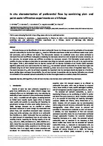
4. Results 4.1. Subsurface Flow Response With and Without Pipe Flow [16] We used the rainfall-runoff event on 25 January 1993 to calibrate Hill-vi including the pipe flow routine. This event produced 23.2 mm of runoff at the hillslope trench after 55.8 mm rainfall. The maximum rainfall intensity of a nearby tipping bucket rain gauge was 10 mm h1 and generated a peak subsurface flow of 3.4 mm h1. This corresponded to specific discharge of 944 l s1 km2 and shows the extreme flashy nature of this hillslope, with very high peak discharge production. Hill-vi was not able to reproduce the measured discharge without activating pipe flow routine using a realistic range of parameters for peak runoff reproduction (Table 2 and Figure 1). The overall model performance was calculated with the Nash-Sutcliffe efficiency and the root mean square error (RMSE) (Table 2). Since the definition of the pipe flow system involved three random variables (as described in Section 3.2), 20 realizations were simulated with the same parameters but with different pipe network geometries in each realization. These ensembles were analyzed statistically (mean and coefficient

of variation) and are shown as a minimum and maximum range in the Figure 1 to view the impact of the pipe flow network geometry on hillslope flow and transport. [17] The simulated runoff from the model that included pipe flow in the model structure adequately captured the measured hydrograph response in terms of peak flow, total runoff, high efficiency and low RMSE (Table 2 and Figure 1). For this event, pipe flow contributed a significant amount of 45% to peak flow and 49% to total runoff. Hillslope runoff is plotted on a logarithmic scale in Figure 1b and shows that the simulation with pipe flow was able to capture the extreme runoff response stretching over three orders of magnitude and the following hydrograph recession. [18] The model was validated on two other events (7 April 1993 and 24 March 1995) and on a continuous time series of several weeks (24 March 1995 to 10 May 1995). This validation procedure ensured that the model was able to simulate the hillslope response for different rainfall event characteristics and for different runoff responses. For the event on 7 April 1993, peak flow was delayed slightly and underestimated. Notwithstanding, peak flow simulations were still nearly twice as high as the simulations using the model without pipe flow. The model Table 2. Model Calibration Event on 25 January 1993a Simulation With Pipes Criteria RMSE, mm h1 Efficiency Efficiency (log(q)) Peak flow, mm h1 Total Pipe Runoff, mm Total Pipe Preevent water, % Peak flow Total flow

5 of 13

a

Simulation Without Pipes

x

CV, %

-

0.39 0.732 0.929

0.11 0.979 0.964

4.29 0.18 0.22

3.43 -

1.98 0.0

3.09 1.40

0.97 7.01

23.18 -

22.65 0.0

23.55 11.58

0.19 7.31

-

80.6 83.1

82.2 85.1

0.32 0.32

Observations

Duration 60 hours and 55.8 mm rainfall.

W03403


Figure 1. Comparison of measured and simulated subsurface flow for the calibrated storm event on 25 January 1993. performance for the simulations with pipe flow was adequate (Table 3) and the overall response was well captured (Figure 2a). [19] The simulation of the second event (24 March 1995) with 43.2 mm of rainfall produced a relatively small runoff response compared to the calibration event shown in Figure 2b. The performance results are listed in Table 4. The simulations without pipe flow again significantly under predicted peak flow and resulted in low performance measures. The simulations with pipe flow captured the runoff response in terms of overall model performance and peak response. Analysis of the simulated continuous time series (24 March 1995 to 10 May 1995) including pipe flow showed that the model performed well (RMSE = 0.12 mm h1 and E = 0.77) in particular compared to the simulation without pipe flow (RMSE = 0.19 mm h1 and E = 0.49). A graphical comparison (not shown due to space restrictions) also confirmed that the low flow in between events and the response to smaller events was well captured. [20] Another interesting aspect of the model calibration and validation analysis is shown by the ensembles generated with the different pipe network geometries. In Figures 1 and 2, the range of runoff response among the ensembles was narrow, indicating insensitivity to specific pipe placement. The coefficient of variation for the model performance measures and for the total runoff and peak flow in Tables 2–4 was always very low (