Preliminary Tests of Multiscale Modeling with a Two-Dimensional ...

MARCH 2005

JUNG AND ARAKAWA

649

Preliminary Tests of Multiscale Modeling with a Two-Dimensional Framework: Sensitivity to Coupling Methods JOON-HEE JUNG*

AND

AKIO ARAKAWA

Department of Atmospheric Sciences, University of California, Los Angeles, Los Angeles, California (Manuscript received 7 October 2003, in final form 10 August 2004) ABSTRACT Preliminary tests of the multiscale modeling approach, also known as the cloud-resolving convective parameterization, or superparameterization, are performed using an idealized framework. In this approach, a two-dimensional cloud-system resolving model (CSRM) is embedded within each vertical column of a general circulation model (GCM) replacing conventional cloud parameterization. The purpose of this study is to investigate the coupling between the GCM and CSRMs and suggest a revised method of coupling that abandons the cyclic lateral boundary condition for each CSRM used in the original cloud-resolving convective parameterization. In this way, the CSRM extends into neighboring GCM grid boxes while sharing approximately the same mass fluxes with the GCM at the borders of the grid boxes. With the original and revised methods of coupling, numerical simulations of the evolution of cloud systems are conducted using a two-dimensional model that couples CSRMs with a lower-resolution version of the CSRM with no physics [large-scale dynamics model (LSDM)]. The results with the revised method show that cloud systems can propagate from one LSDM grid column to the next as expected. Comparisons with a straightforward application of a single CSRM to the entire domain (CONTROL) show that the biases of the large-scale thermodynamic fields simulated by the coupled model are significantly smaller with the revised method. The results also show that the biases are near the smallest when the velocity fields of the LSDM and CSRM are nudged to each other with the time scale of a few hours and the thermodynamic field of the LSDM is instantaneously updated at each time step with the domain-averaged CSRM field.

1. Introduction It has been well recognized that cumulus convection plays a central role in the maintenance and evolution of the atmosphere. To represent the statistical effects of the cumulus convection, a number of parameterization schemes have been proposed during the last decades for use in weather prediction and climate simulation models [see, e.g., Emanuel and Raymond (1993) for a review]. In spite of the accumulated achievements, however, there are still a number of uncertainties in modeling cloud and associated processes and in formulating their overall effects on the large-scale environment (e.g., Arakawa 2000, 2004; Randall et al. 2003). Moreover, as emphasized by Arakawa (2004) and Jung and Arakawa (2004), there are even conceptual problems in existing formulations of model physics in * Current affiliation: Department of Atmospheric Science, Colorado State University, Fort Collins, Colorado. Corresponding author address: Dr. Joon-Hee Jung, Department of Atmospheric Science, Colorado State University, Fort Collins, CO 80521-9990. E-mail: [email protected]

© 2005 American Meteorological Society

MWR2878

large-scale models. One is that different physical processes can interact only through grid-scale prognostic variables of the models because of their modular structure, missing most of small-scale direct interactions between the processes. Another is that existing formulations of model physics do not converge to the local and instantaneous real physics as the resolution is refined. This is because the governing equations are modified, rather than approximated, through the use of parameterized expressions for model physics. One of the future emphases in climate modeling should therefore be on developing a unified formulation of the entire spectrum of the interactions between different physical processes, with which the convergence problem is eliminated. Arakawa (2000, 2004) discussed two possible approaches to unify the model physics: the “parameterize everything” approach, in which all formulations of model physics are made in the continuous form before discretization is introduced so that the concept of subgrid-scale parameterization is abandoned, and the “resolve everything” approach, in which the entire globe is covered by a large-eddy simulation (LES) model of turbulence with detailed formulations of cloud microphysics and radiation. To be practical, however, we can think of a compromised target

650

MONTHLY WEATHER REVIEW

along the line of the resolve everything approach: that is, covering the entire globe with a cloud-system resolving model (CSRM) in which all sub-cloud-scale processes such as cloud microphysics, radiation, and turbulence are still parameterized. Recently, Grabowski and Smolarkiewicz (1999) and Grabowski (2001) proposed an approach called cloudresolving convective parameterization (CRCP) for GCMs, which is close to the resolve everything approach in spirit. In this approach, subgrid scales are represented by a two-dimensional CSRM embedded within each column of a GCM. As in existing convection parameterizations, the GCM provides large-scale advective tendencies as forcing to the CSRMs, while the CSRMs calculate the convective response to the forcing. The thermodynamic fields of GCM are then updated with the domain averages of the predicted fields of CSRM. Khairoutdinov and Randall (2001; see also Randall et al. 2003) applied this parameterization, called by them superparameterization, to the climate simulation problem. The results presented by them are very encouraging especially because almost no tuning was done. The simulation needed two orders of magnitude more computer time than with conventional parameterization even though the CSRM used was highly simplified. Yet the approach is promising for future climate models because it will eventually play the role of a “physics coupler” that enables us to treat all interacting physical processes within a unified framework, which we call a multiscale modeling framework (MMF). Despite the great promise of the new approach, there are a number of problems to be solved (Randall et al. 2003) before its merit can be fully appreciated. In particular, we note that the cloud-resolving convective parameterization, or superparameterization, as originally proposed has the following weaknesses: 1) Because of the use of a cyclic lateral boundary condition for each CSRM, CSRMs for neighboring GCM grid boxes can communicate only through the GCM. 2) Also because of the use of a cyclic lateral boundary condition, each CSRM converges to a 1D cloud model as the GCM grid size approaches the CSRM grid size, with no CSRM vertical velocity on which CSRM physics is based. 3) The two-dimensionality of the CSRM on which the parameterization is based is obviously an artificial constraint. Problem 1 was recognized in Grabowski (2001). In that paper, Grabowski compared CRCP simulations using different horizontal resolutions of the large-scale model (and different sizes of the CRCP domain) against the fully cloud-resolving counterpart. Based on these results, he speculated that the limitation of CRCP in the mesoscale range is caused by the inability of

VOLUME 133

small-scale features to propagate coherently from one large-scale model column to another. Because the new MMF approach is extremely computer demanding, we believe that a simple framework should be used as much as possible to find the most satisfactory way of implementing it. In this paper we suggest a revised coupling method that can overcome weaknesses 1 and 2 of the original method. There is the possibility of using the revised method in the quasi-3D MMF (see Arakawa 2004 and Randall et al. 2003 for more details) that partially overcomes weakness 3. We then investigate the sensitivity of the results to coupling methods using an idealized framework. The paper is organized as follows. Section 2 describes the original and revised methods of coupling. Section 3 describes an idealized coupled model that can illustrate the MMF approach and control experiments that are used for initialization and validation of the coupled model. Sections 4 and 5 present the results of the experiments and discuss the sensitivity of the results to coupling methods. Finally, section 6 presents a summary and conclusions.

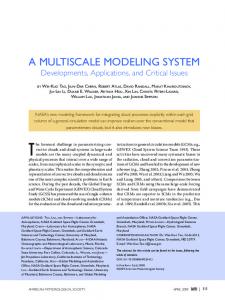
2. Methods of coupling between a GCM and CSRMs a. Original method: Confined CSRMs Grabowski and Smolarkiewicz (1999) and Grabowski (2001) discussed the coupling formalism of the original method in detail. Here we describe only its main features. In this coupling, a 2D CSRM is embedded within each GCM column with a cyclic lateral boundary condition. Figure 1a presents a schematic illustration of the coupling method. In the coupled system, the GCM equation is represented by D⌿ ⫽ S⌿ ⫹ F⌿, Dt

共1兲

where ⌿ is an arbitrary prognostic variable of the GCM, D/Dt ⬅ ⳵/⳵t ⫹ U · 䉮, U ⫽ (U,V,W ) is the largescale flow resolved by the GCM, S⌿ is the source of ⌿ explicitly represented by the GCM, and F⌿ is the source of ⌿ due to processes that can only be resolved by the CSRM. Similarly, the CSRM equation is represented by

FIG. 1. Schematic illustrations of the coupling methods between GCM and CSRM in the MMF. See text for further explanation.

MARCH 2005

d␺ ⫽ s␺ ⫹ f␺, dt

共2兲

where ␺ is an arbitrary prognostic variable of the CSRM, d/dt ⬅ ⳵/⳵t ⫹ u · 䉮, u ⴔ (u,v,w) is the smallscale flow resolved by the CSRM, s␺ is the source due to all physical processes in the CSRM, and f␺ represents the forcing of the CSRM by the GCM. For a thermodynamic variable (Q or q; temperature, water vapor or hydrometeors), the source of Q in the GCM due to small-scale processes is given by FQ ⫽

冓 冔

dq , dt

共3兲

where dq/dt is given by (2) and the 具典 denotes the horizontal average over each CSRM domain. The forcing of the CSRM by the GCM for the variable q is, on the other hand, given by fq ⫽ ⫺U · ⵜQ.

共4兲

In Fig. 1(a), the upward thin solid arrows represent FQ and the downward heavy solid arrows represent fq. In practice, they implemented this coupling through updating the large-scale thermodynamic fields by the horizontal averages of the CSRM fields (Grabowski and Smolarkiewicz 1999). For the zonal velocity (U or u), the sources in the GCM and CSRM are given by FU ⫽ ⫺

651

JUNG AND ARAKAWA

U ⫺ 具u典 具u典 ⫺ U and fu ⫽ ⫺ , ␶m ␶m

共5兲

respectively, where ␶m is the nudging time scale. In the figure, the dashed arrows represent nudging of the velocity components of the GCM and the domainaveraged velocity components of the CSRMs with each other. In this method, the communication between the GCM and CSRMs occurs only at the center of the GCM column, and there is no direct communication between the CSRMs in neighboring GCM grid boxes because of the cyclic lateral boundary condition imposed on them.

b. Revised method: Extended CSRMs Figure 1b presents a schematic illustration of the revised method we test in this paper. In this coupling, the cyclic lateral boundary condition of the CSRMs is abandoned so that the CSRMs at neighboring GCM grid boxes are coupled at the open dot points in the figure. Accordingly, convective systems can propagate from one GCM grid box to the next. In the revised method, the thermodynamic variables of the GCM are nudged to those of the CSRM with a time scale (␶t): FQ ⫽ ⫺

Q ⫺ 具q典 . ␶t

共6兲

Thus, the instantaneous updating used in the original method can be interpreted as the limiting case ␶t → 0. The velocity components of the GCM and CSRMs are coupled through FU ⫽ ⫺

U ⫺ 具u典 u ⫺ U* and fu ⫽ ⫺ , ␶m ␶m

共7兲

where U* is the GCM velocity component interpolated to each CSRM grid point. The coupling through FU and fu is shown by the dashed arrows in Fig. 1b. If this coupling is very strong, communication between the CSRMs at neighboring GCM grid boxes is through the GCM, rather than by the CSRMs themselves; this is a situation analogous to the original method. The main point of the revised method is that the GCM and CSRMs share approximately the same horizontal mass fluxes at the open dot points in Fig. 1b so that CSRMs can directly recognize large-scale horizontal velocity, including its convergence, predicted by the GCM. Also, since the cyclic lateral boundary condition is abandoned, CSRMs recognize large-scale gradients of thermodynamic variables beyond the GCM grid size. In this way, the CSRMs can recognize large-scale thermodynamic advective forcing by themselves, not through the forcing by the GCM given by fq. (Thus, fq is not relevant in this method.)

3. The model and control experiments a. The model To test the coupling methods described in section 2, we set up a two-dimensional framework that couples CSRMs with a lower-resolution version of the CSRM with no physics [large-scale dynamics model (LSDM)], which mimics the role of a GCM in actual implementations of the MMF framework. The CSRM we use is a nonhydrostatic anelastic model originally developed by Krueger (1988). The physical parameterizations in the model include a thirdmoment turbulence closure (Krueger 1988), a diagnostically determined turbulence length scale (Xu and Krueger 1991), a scheme for turbulence-scale condensation (Chen 1991), a three-phase microphysical parameterization (Krueger et al. 1995a; Lord et al. 1984), and an advanced radiative transfer parameterization (Fu et al. 1995; Krueger et al. 1995b). The model has been extensively applied to a variety of cloud regimes including stratocumulus, altocumulus, cumulonimbus, and cirrus clouds (see, e.g., Krueger 2000). The model has also been used to investigate the resolution dependence of model physics required for low-resolution models to accurately predict averaged fields (Jung and Arakawa 2004).

b. Control experiments In this study, we first apply the CSRM with a 2-km horizontal grid size to a 512-km horizontal domain. In

652

MONTHLY WEATHER REVIEW

the vertical, the model has 34 levels based on a stretched grid with a top at 18 km. The vertical grid size ranges from about 100 m near the surface to about 1000 m near the model top. The upper and lower boundaries are rigid and the lateral boundaries are cyclic. Two types of idealized surface conditions are used: land and ocean. Over land, diurnal cycles are included with the ground wetness set to 75%. There is no diurnal variation over ocean with a prescribed temperature of 299.7 K. In this case, the cosine of the solar zenith angle is fixed to 0.5, representing a typical daytime condition in the Tropics. The initial thermodynamic state and horizontal wind fields are based on the Global Atmospheric Research Program (GARP) Atlantic Tropical Experiment (GATE) Phase-III mean sounding. Clouds are initiated by small random temperature perturbations introduced into the lowest model layer over the 15-min period after the first 5 min of the integration. The Coriolis parameter for 15°N is used. Large-scale forcing representing climatological background is imposed on the model in one of two ways depending on the experiments we performed. One way is through prescribed cooling and moistening rates (Fig. 2a) and the other is through prescribing large-scale vertical velocity. The prescribed vertical velocity varies in the model domain as w共x, z兲 ⫽ 1.7 · A共z兲 · cos 2␲

冉

冊

x ⫹ XⲐ2 , X

共8兲

where X is the horizontal domain size and A(z) is shown in Fig. 2b. As control experiments (Control), we perform integrations of the CSRM under the land surface condition with prescribed advective cooling and moistening (CTL-A) and under the ocean surface condition with prescribed vertical velocity (CTL-B). Each of them is

FIG. 2. Vertical profiles of the prescribed (a) large-scale advective cooling and moistening rates used in the experiments discussed in sections 3, 4, and 5a and (b) the amplitude of large-scale vertical velocity used in the experiment discussed in section 5b. Here, the moistening rate is multiplied by L/cp where L and cp are the latent heat of condensation and the specific heat of dry air, respectively.

VOLUME 133

13 days long with a 10-s time step. Selected snapshots from the last 10-day integrations of CTL-A and CTL-B are used for initialization and validation of the MMF experiments. As an example of Control, development of cloud systems for a 1-h period from CTL-A is presented in Fig. 3. More results from Control are presented in sections 4 and 5 along with those from the MMF experiments. Figure 3 shows cross sections of cloudiness (light gray), precipitation (dark gray), and wind (arrows) at 1200 and 1300 local time. In the figure the zonal average of the zonal wind component is removed from the wind field. The figure exhibits aligned shallow clouds in the lower troposphere, stratiform clouds in the upper troposphere, and precipitating convective systems penetrating through the troposphere. During this period the deep convective systems near x ⫽ 64 and 448 km decay and a new system develops near x ⫽ 384 km. These evolutions of cloud systems are compared with those of the MMF experiments described in section 4.

4. MMF experiments: Sensitivity to the coupling methods In this section, we compare the MMF results obtained with each of the two different coupling methods described in section 2. The main purpose of the experiments described here is to see the impact of the cyclic lateral boundary condition imposed to each CSRM in the original method. The CSRMs used in the MMF are the same as that used in Control, with the horizontal grid size of 2 km, except that they are embedded in LSDM grids. The LSDM used in the MMF is configured in the following way: The model domain is 512 km ⫻ 18 km as in Control. Horizontal grid size is either 16 or 64 km. Like the CSRM, the LSDM has 34 levels based on a stretched vertical grid ranging from about 100 m near the surface to about 1000 m near the model top. The upper and lower boundaries are rigid and the lateral boundaries are cyclic. The LSDM has no physics. The MMF is initialized using a selected realization from CTL-A and run for a 1-day period. In both coupling methods, the time scale for nudging the horizontal velocity fields is set to 1 h and the thermodynamic variables of the LSDM are instantly updated by horizontal averages of the CSRM fields. To visualize the sensitivity of MMF simulations to the coupling methods, we first present results from short integrations from the realization of CTL-A shown in the upper panel of Fig. 3. Figure 4a shows the vertical cross sections of moist static energy from CTL-A after 1 h, which corresponds to the lower panel of Fig. 3. It appears that the area with high moist static energy in the lower troposphere is associated with the aligned shallow clouds, and the area of high moist static energy connecting the lower and upper troposphere is associ-

MARCH 2005

JUNG AND ARAKAWA

653

FIG. 3. Vertical cross sections of cloudiness, precipitation, and wind at (a) 1200 and (b) 1300 local time obtained from the control simulation with 2-km horizontal grid size (CTL-A). The areas of higher cloudiness than 0.5 are shaded light gray, and the mixing ratios of rain, snow, and graupel larger than 0.1 g kg⫺1 are indicated with dark gray. Winds are shown with arrows.

ated with the deep convective system that appears in the lower panel of Fig. 3 near x ⫽ 384 km. Corresponding results from MMF integrations with the original method are shown in Fig. 4b. In these results, the newly developed deep convective system near x ⫽ 384 km is simulated very poorly for both 16- and 64-km grid sizes of the LSDM, while the broad area with high moist static energy in the lower troposphere is relatively well simulated. With the revised method shown in Fig. 4c, on the other hand, the deep convective system is well simulated even with the 64-km grid size of the LSDM. Next, we present the vertical cross sections of upward mass fluxes obtained from CTL-A and the MMF integrations with the two coupling methods (Fig. 5). These are the results of 20-min integrations from a late afternoon realization of CTL-A. Figure 5a for CTL-A shows that strong upward mass fluxes are present only in narrow regions of the model domain. Weak downward fluxes are generally present in the rest of the domain. With the original method (Fig. 5b), upward mass fluxes are either more evenly distributed as in the case of 64-km LSDM grid size or weaker than those of CTL-A as in the case of 16-km LSDM grid size. The cyclic lateral boundary condition imposed to each CSRM in the original method requires that the mean vertical mass flux over each LSDM grid interval be zero, that is, the upward and downward mass fluxes must be bal-

anced within each interval. Then, since the CSRM physics recognizes mass fluxes simulated by the CSRM rather than GCM mass fluxes, the convective system tends to be horizontally trapped within a single LSDM grid interval and less developed as we can see in Fig. 4b. Such an effect becomes more visible as the LSDM grid size decreases. In the revised method, on the contrary, the horizontal resolution of the LSDM hardly affects the performance of the simulation. Figure 6 shows Hovmöller diagrams (x–t) of the cloud-top temperature for a simulated day. Following Xu and Krueger (1991), the cloud top is defined as the layer where the path of liquid water and ice [i.e., 兰(ql ⫹ qi) ␳dz] first exceeds 0.1 kg m⫺2 when integrated downward from the model top, where ql is the mixing ratio of liquid water and qi is that of ice. In the figure, cirrus anvils associated with cumulonimbi appear white and there are no optically thick clouds in dark areas. In CTL-A (Fig. 6a), we see organized cloud systems propagating westward. In the MMF integration using the original method (Fig. 6b), on the other hand, the organized cloud systems do not steadily propagate with the 16-km horizontal grid size (upper panel) and are almost completely trapped within a single LSDM grid interval with the 64-km grid size. We note that the propagation that appears with the 16-km grid size is entirely through the LSDM rather than direct commu-

654

MONTHLY WEATHER REVIEW

FIG. 4. Vertical cross sections of moist static energy divided by cp obtained from (a) Control (CTL-A) and the MMF experiments with the (b) original and (c) revised methods using (upper) 16- and (lower) 64-km horizontal grid sizes of the LSDM. The areas with higher values than 336 K are shaded. Contour interval is 2 K. The dashed lines in (b) and (c) represent the LSDM grids.

VOLUME 133

MARCH 2005

JUNG AND ARAKAWA

655

FIG. 5. Upward mass fluxes obtained from (a) Control (CTL-A) and the MMF experiments using the (b) original and (c) revised methods, with (upper) 16- and (lower) 64-km horizontal grid sizes of the LSDM. The vertical dashed lines in (b) and (c) indicate the LSDM grids.

nications between neighboring CSRMs. With the revised method (Fig. 6c), the development of the organized cloud systems and the propagation of cloud systems are both well simulated. Although we have so far compared the results of integrations from a single realization, we are naturally interested in the systematic impact of the cyclic lateral boundary condition on many realizations. Figure 7 shows the biases of the ensemble- and domainaveraged profiles of moist static energy (upper panels) and total water (lower panels). Here, the ensemble consists of 10 sets of 1-day integrations. To construct this figure, we first calculate the bias of 1-day MMF integration by comparing it with that of Control. Ensemble and domain averages are then taken. With the original coupling method (Figs. 7a and 7c), there are deficits of

moist static energy and total water in the middle to upper troposphere and surpluses in the lower troposphere. Such biases in the thermodynamic fields seem to reflect the lack of strong deep convection, which is responsible for the upward transport of moist static energy and total water from the surface in Control. With the revised method (Figs. 7b and 7d), the biases are relatively small for both moist static energy and total water.

5. MMF experiments: Sensitivity to the coupling strengths In the previous section, we discussed the problems caused by the cyclic lateral boundary condition for the CSRMs used in the originally proposed CRCP and pre-

656

MONTHLY WEATHER REVIEW

VOLUME 133

FIG. 6. Hovmöller diagrams (x–t) of cloud-top temperature obtained from (a) Control (CTL-A) and the MMF experiments using the (b) original and (c) revised methods with (upper) 16- and (lower) 64-km horizontal grid sizes of the LSDM. The vertical dashed lines in (b) and (c) indicate the LSDM grids.

sented a revised coupling method that can eliminate such problems. In practice, these couplings can be achieved through a proper nudging of the variables between the GCM and CSRMs. As a preliminary test for real applications of the MMF using the revised method, we now investigate the sensitivity of the results to the coupling strengths, that is, the time scales for nudging thermodynamic variables (␶t) and velocity (␶m).

a. Sensitivity to the time scales for nudging thermodynamic variables (␶t) Figure 8 shows the biases of the ensemble- and domain-averaged profiles of moist static energy, total water, temperature, and relative humidity. This figure is constructed in the same way as in Fig. 7 but with different time scales (␶t) for nudging thermodynamic vari-

ables of the LSDM to those of the CSRM averaged over each LSDM grid interval. Here, the time scale for nudging the velocity fields (␶m) is fixed to 1 h and the grid size of the LSDM is 64 km. When ␶t ⬎ 0, thermodynamic variables of the LSDM are predicted not only by the CSRM but also by LSDM’s own advection and grid-scale saturation adjustment processes. The simulated results are quite sensitive to the nudging time scale. The bias is near minimum when the thermodynamic fields of the LSDM are instantly updated (␶t ⬃ 0) with the domain-averaged CSRM fields. When the nudging time scale is long, the biases clearly reflect the lack of strong deep convection in the system, such as deficit and surplus of moist static energy in the upper and lower troposphere, respectively, surplus of total water in the whole troposphere, and cold and humid atmosphere.

MARCH 2005

JUNG AND ARAKAWA

657

FIG. 7. Biases of the ensemble- and domain-averaged profiles of (upper) moist static energy divided by cp and (lower) total water multiplied by L/cp obtained from the MMF experiments using the (left) original and (right) revised methods.

b. Sensitivity to the time scales for nudging velocity (␶m) One of the major benefits of the revised method is that the GCM and CSRMs share approximately the same mass fluxes at the border of GCM grid boxes so that CSRMs can directly recognize large-scale velocity predicted by the GCM. Unlike the real GCM, however, the LSDM we use is a 2D model and covers a relatively small horizontal domain so that it cannot predict a complete large-scale velocity field. Therefore, the effect of background velocity field that cannot be predicted by the LSDM is prescribed as was done in the previous experiments. For the experiments discussed in this section, however, large-scale vertical velocity, rather than large-scale advective cooling and moistening rates, is prescribed. The CSRM then recognizes this background vertical velocity through corresponding background horizontal velocity gradient. In this framework, therefore, a combination of the LSDM-simulated ver-

tical velocity and the prescribed background vertical velocity mimics the vertical velocity of a real GCM. Following this idea, we first prescribe a background vertical velocity for the control, CTL-B, as shown by (8). The same background vertical velocity is also used for the LSDM. The CSRM then recognizes this background vertical velocity indirectly through corresponding background horizontal velocity, Ub, along with the zonal velocity predicted by the LSDM. In this case, (7) becomes 共ULSDM ⫹ Ub兲 ⫺ 具u典 and ␶m u ⫺ 共U* LSDM ⫹ U* b兲 fu ⫽ ⫺ , ␶m

FU ⫽ ⫺

共9兲

where ULSDM is the zonal velocity predicted by the LSDM and U* is the linearly interpolated value of U on each CSRM grid. This rather elaborate procedure is

658

MONTHLY WEATHER REVIEW

VOLUME 133

FIG. 8. Sensitivity to the time scales for nudging thermodynamic variables on biases of the ensemble- and domain-averaged profiles: (a) moist static energy divided by cp, (b) total water multiplied by (L/cp), (c) temperature, and (d) relative humidity, obtained from the MMF experiments with 64-km horizontal grid size of the LSDM. Here, the time scale for nudging velocity fields is fixed to 1 h.

adopted in view of our objective of studying the sensitivity of MMF results to the time scale ␶m for nudging horizontal velocity. Whether a choice of ␶m is appropriate or not, therefore, can be judged by seeing how well the CSRMs used in the MMF can simulate the thermodynamical response to the inhomogeneous horizontal velocity field. Below we present the results of the MMF integrations designed in the way described above to test the sensitivity of the results to the coupling strengths, that is, the time scale ␶m for nudging the velocity field. Figure 9 shows Hovmöller diagrams (x–t) of the cloud-top temperature for a day from (a) CTL-B and the MMF integrations using the revised method for the (b)–(d) 16- and (e)–(g) 64-km horizontal grid sizes of the LSDM with the following time scales for nudging horizontal velocity fields: 10 min, 1 h, and 6 h. In these integrations, the thermodynamic fields of the LSDM are instantly updated by the domain averages of the CSRM fields at every time step, that is, ␶t ⬃ 0. With the 16-km horizontal grid size of the LSDM, the results are not very sensitive to ␶m because the LSDM dynamics with the relatively fine resolution is close to that of the

CSRM. With the 64-km horizontal grid size of the LSDM, on the contrary, the development of cloud systems is weak and more or less confined near the center of the model domain when the time scale (␶m) is short, that is, when the nudging is strong. As the time scale becomes longer, this modulation becomes weaker and thus cloud systems propagate more freely. Figure 10 shows the cross sections of ensembleaveraged moist static energy (left) and its deviation from the zonal mean (right). Here, the grid size of the LSDM is 64 km. The ensemble consists of 10 sets of 1-day integrations. In CTL-B (Fig. 10a), it appears that the cumulus activity is slightly shifted to the west of the domain center even though the most favorable condition is placed at the center through the prescribed background vertical velocity. With the time scale of 1 h (Fig. 10c), the coupled model reproduces a state similar to that of CTL-B. For a shorter time scale—with the time scale of 10 min (Fig. 10b), for example—the deviation of the moist static energy from the zonal mean shows the feature confined to the lower atmosphere. With the time scale of 6 h (Fig. 10d), on the other hand, the zonal variation of the moist static energy becomes weaker.

MARCH 2005

JUNG AND ARAKAWA

659

FIG. 9. Hovmöller diagrams (x–t) of cloud-top temperature obtained from (a) Control (CTL-B) and the MMF experiments with (b), (c), (d) 16- and (e), (f), (g) 64-km horizontal grid sizes of the LSDM. The time scales for nudging velocity fields are 10 min, 1 h, and 6 h. The vertical dashed lines on the figures indicate the separation of the LSDM grids. Here, the thermodynamic variables of the LSDM are instantly updated with those of the CSRM.

These features commonly appear in other thermodynamic fields such as total water, temperature, and relative humidity (not shown). Figure 11 shows the biases of the ensemble- and domain-averaged profiles of thermodynamic fields for different time scales for nudging the velocity field. Here the grid size of the LSDM is 64 km. They again show the sensitivity of the simulated results to the time scale. There is no significant difference between 1 and 6 h, but with the 10-min time scale the result is subject to large biases. In this case, the biases again show the sign of the lack of strong deep convection as we have seen in Fig. 8.

6. Summary and conclusions A new modeling approach was proposed by Grabowski (Grabowski and Smolarkiewicz 1999;

Grabowski 2001), in which a two-dimensional cloudresolving model (CSRM) is embedded in each vertical column of a general circulation model (GCM) to explicitly represent cloud-scale physical processes within that column. This approach, called cloud-resolving convective parameterization (CRCP) by them and superparameterization by Khairoutdinov and Randall (2001), is very promising for use in future climate models because it will eventually play the role of “physics coupler,” which enables us to treat multiscale interactions between physical processes in a unified framework. We call this framework multiscale modeling framework (MMF). There are a number of problems to be solved (e.g., Randall et al. 2003), however, before the merit of the new approach can be fully appreciated. In particular, we note that the CRCP as originally proposed has

660

MONTHLY WEATHER REVIEW

VOLUME 133

FIG. 11. As in Fig. 8, but for sensitivity to the time scales for nudging velocity fields. Here, the thermodynamic variables of the LSDM are instantly updated with those of the CSRM.

FIG. 10. Sensitivity to the time scales for nudging velocity fields on (left) the ensemble-averaged moist static energy divided by cp and (right) its deviation from the zonal mean obtained from (a) Control (CTL-B) and (b), (c), (d) the MMF experiments with 64-km horizontal grid size of the LSDM. The time scales for nudging velocity fields are (b) 10 min, (c) 1 h, and (d) 6 h. The areas with higher values than 338 K are shaded. Thick and thin lines in the right panels show positive and negative values, respectively. Here, the thermodynamic variables of the LSDM are instantly updated with those of the CSRM.

weaknesses in the method of coupling the GCM and CSRMs. In the original method, CSRMs in neighboring GCM grid boxes can communicate only through the GCM because of the use of a cyclic lateral boundary condition for each CSRM. Also because of the use of the lateral boundary condition, each CSRM converges to a 1D cloud model with no vertical velocity as the GCM grid size approaches the CSRM grid size.

We suggest in this paper a revised coupling method that can overcome these weaknesses. In the revised method, the cyclic lateral boundary condition is abandoned so that the CSRMs in neighboring GCM grid boxes are directly coupled at the borders of the GCM grid boxes. The GCM and CSRMs share approximately the same mass fluxes at the borders through nudging their horizontal velocities with each other. Since there is no cyclic lateral boundary condition, CSRMs can recognize large-scale gradients of thermodynamic variables beyond the GCM grid interval. In these ways, the CSRMs can recognize large-scale advective forcing by themselves. This is advantageous from the point of view of convergence of the coupled system as the GCM grid size approaches that of the CSRM. As a preliminary test for applications of the MMF approach, we have investigated the sensitivity of the results to the architecture of the coupling using an idealized framework that couples CSRMs with a largescale dynamics model (LSDM), which is a lowerresolution version of the CSRM without physics. For control experiments (Control), we run the CSRM with a 2-km horizontal grid size for 1) the land surface condition with prescribed background advective cooling and moistening rates (CTL-A), and 2) the ocean surface condition with prescribed background vertical velocity (CTL-B). Realizations selected from the integrations of CTL-A and CTL-B are used for initialization and validation of the MMF integrations.

MARCH 2005

661

JUNG AND ARAKAWA

The sensitivity tests to the methods of coupling show that deep convective systems develop less with the original method and they propagate only when the grid size of the LSDM is very small. Spurious effects are generated because of the cyclic lateral boundary condition that influences even the ensemble- and domainaveraged profiles of predicted large-scale thermodynamic fields. We have found that, with the revised method of coupling, cloud systems propagate properly with no spurious effects due to the cyclic lateral boundary condition. Moreover, biases on large-scale thermodynamic fields are smaller with the revised method and the horizontal resolution of the LSDM hardly affects the performance of the results. This paper also presents the results of sensitivity tests to the strength of coupling represented by time scales for nudging the thermodynamic fields and the velocity between the LSDM and CSRMs. Especially for the sensitivity test to the time scale for nudging the velocity, background vertical velocity, rather than background advective cooling and moistening rates, is prescribed. The CSRM recognizes this background vertical velocity through corresponding background horizontal velocity. The CSRM thus recognizes the sum of the horizontal velocity predicted by the LSDM and the background horizontal velocity as “large scale” horizontal velocity. In these tests, therefore, a combination of the LSDM and the prescribed background velocity mimics a real GCM. This rather elaborate procedure is adopted in view of our objective of studying the sensitivity of MMF results to the time scale of nudging horizontal velocity. The test results show that the biases are near minimum when the thermodynamic field of the LSDM is instantly updated with the domain-averaged CSRM thermodynamic field and the velocity fields are nudged toward each other using a time scale of a few hours. The optimum time scale of a few hours for nudging velocity fields is probably associated with the time scale for small-scale convective process to adjust itself to largescale advective process. The choice of optimum time scales for nudging in the MMF approach is not a simple problem, although fortunately the sensitivity to the choice does not seem to be great if it is in the right range. In the future, perhaps we should use a more general formulation of nudging, such as the use of different time scales for nudging the CSRM velocity to the GCM velocity and for nudging the GCM velocity to the CSRM velocity. Though it may sound technical, the problem we have is closely related to the scientific problem of mutual adjustment of different scales and that of different fields in the atmosphere. We note that the choice of adjustment time scales has been and still is one of the major issues in conventional cumulus parameterizations. The importance of that issue does not change even in the MMF approach, in which CSRMs are used as a parameterization in the sense that only their bulk results influence large-scale

dynamics. There are important differences between the conventional and MMF approaches because many of the other uncertainties in the former approach are eliminated in the latter approach. In particular, the effects of cloud-scale interactions are included in the MMF approach and the system converges to the straightforward application of the CSRM to the entire globe, as the resolution is refined. To establish an optimum architecture for the MMF, however, sensitivity studies such as those presented in this paper should be performed with a 3D framework, perhaps using the quasi-3D MMF discussed in Arakawa (2004). Finally, we emphasize that existing CSRMs are far from perfect models, although in this paper we pretended as if it is the case. A significant part of our modeling efforts, therefore, may have to be diverted to improvement of CSRMs in the future. One of the most important merits of the MMF approach is that verifications against observations can be done on multiscales: through CSRM results for cloud and mesocales and through GCM results for synoptic and planetary scales. Acknowledgments. We wish to thank David Randall, Steven Krueger, and two anonymous reviewers for extensive comments on the original manuscript. This research is supported by NSF Grant ATM-0071345, NASA Grant RSP-0248-0017, and DOE Grant DEFG02-02ER63370. REFERENCES Arakawa, A., 2000: Future development of general circulation models. General Circulation Model Development: Past, Present, and Future, D. A. Randall, Ed., Academic Press, 721–780. ——, 2004: The cumulus parameterization problem: Past, present, and future. J. Climate, 17, 2493–2525. Chen, J.-M., 1991: Turbulence-scale condensation parameterization. J. Atmos. Sci., 48, 1510–1512. Emanuel, K. A., and D. J. Raymond, Eds., 1993: The Representation of Cumulus Convection in Numerical Models. Meteor. Monogr., No. 46, Amer. Meteor. Soc., 246 pp. Fu, Q., S. K. Krueger, and K. N. Liou, 1995: Interactions of radiation and convection in simulated tropical cloud clusters. J. Atmos. Sci., 52, 1310–1328. Grabowski, W. W., 2001: Coupling cloud processes with the largescale dynamics using the cloud-resolving convective parameterization (CRCP). J. Atmos. Sci., 58, 978–997. ——, and P. K. Smolarkiewicz, 1999: CRCP: A cloud resolving convective parameterization for modeling the tropical convective atmosphere. Physica D, 133, 171–178. Jung, J.-H., and A. Arakawa, 2004: The resolution dependence of model physics: Illustrations from nonhydrostatic model experiments. J. Atmos. Sci., 61, 88–102. Khairoutdinov, M. F., and D. A. Randall, 2001: A cloud-resolving model as a cloud parameterization in the NCAR Community Climate System Model: Preliminary results. Geophys. Res. Lett., 28, 3617–3620. Krueger, S. K., 1988: Numerical simulation of tropical cumulus clouds and their interaction with the subcloud layer. J. Atmos. Sci., 45, 2221–2250. ——, 2000: Cloud system modeling. General Circulation Model

662

MONTHLY WEATHER REVIEW

Development: Past, Present, and Future, D. A. Randall, Ed., Academic Press, 605–640. ——, Q. Fu, K. N. Liou, and H.-N. Chin, 1995a: Improvements of an ice-phase microphysics parameterization for use in numerical simulations of tropical convection. J. Appl. Meteor., 34, 281–287. ——, G. T. McLean, and Q. Fu, 1995b: Numerical simulation of the stratus-to-cumulus transition in the subtropical marine boundary layer. Part I: Boundary-layer structure. J. Atmos. Sci., 52, 2839–2850.

VOLUME 133

Lord, S. J., H. E. Willoughby, and J. M. Piotrowicz, 1984: Role of a parameterized ice-phase microphysics in an axisymmetric, nonhydrostatic tropical cyclone model. J. Atmos. Sci., 41, 2836–2848. Randall, D., M. Khairoutdinov, A. Arakawa, and W. Grabowski, 2003: Breaking the cloud parameterization deadlock. Bull. Amer. Meteor. Soc., 84, 1547–1564. Xu, K.-M., and S. K. Krueger, 1991: Evaluation of cloudiness parameterizations using a cumulus ensemble model. Mon. Wea. Rev., 119, 342–367.