aDepartment of Electrical Engineering, California Institute of Technology ..... the best possible sojourn time tail behavior under heavy-tailed job size distributions ...
Performance Evaluation Performance Evaluation 00 (2010) 1–22
Tail-robust Scheduling via Limited Processor Sharing Jayakrishnan Naira , Adam Wiermanb , Bert Zwartc a Department
of Electrical Engineering, California Institute of Technology and Mathematical Sciences Department, California Institute of Technology c CWI Amsterdam, VU University Amsterdam, Eurandom & Georgia Tech
b Computing
Abstract From a rare events perspective, scheduling disciplines that work well under light (exponential) tailed workload distributions do not perform well under heavy (power) tailed workload distributions, and vice-versa, leading to fundamental problems in designing schedulers that are robust to distributional assumptions on the job sizes. This paper shows how to exploit partial workload information (system load) to design a scheduler that provides robust performance across heavy-tailed and light-tailed workloads. Specifically, we derive new asymptotics for the tail of the stationary sojourn time under Limited Processor Sharing (LPS) scheduling for both heavy-tailed and light-tailed job size distributions, and show that LPS can be robust to the tail of the job size distribution if the multiprogramming level is chosen carefully as a function of the load. Keywords: GI/GI/1 queue, scheduling, limited processor sharing, large deviations, tail asymptotics, heavy-tailed job size, light-tailed job size, tail-robustness 1. Introduction In the study of scheduling policies, much of the focus has traditionally been on designing policies that have good performance in expectation. For example, in order to minimize the expected sojourn time (a.k.a. response time, flow time) in a single server queue it is well known that the scheduler should give priority to jobs with small remaining sizes via Shortest Remaining Processing Time (SRPT) [1], which is optimal regardless of the job size distribution and arrival process. However, providing good performance in expectation is not sufficient. It is also important for a scheduler to provide good distributional performance. For example, quality of service guarantees in web applications often rely on specifying guarantees about the tail of the sojourn time distribution, e.g., that 95% of requests will have sojourn time < s seconds. Resultantly, there has been a substantial amount of work in recent years studying the sojourn time distribution, P (V > x) of scheduling policies in a GI/GI/1 setting. Due to the difficulty of an exact distributional analysis, much of this work focuses on understanding the sojourn time tail asymptotics, i.e., the behavior of P (V > x) as x → ∞, which provides a characterization of the
Nair, Wierman and Zwart / Performance Evaluation 00 (2010) 1–22
2
likelihood of large delays. From this work, which we survey briefly in Section 2, has emerged an understanding of how to optimally schedule for the sojourn time tail. Interestingly, unlike when optimally scheduling for the expected sojourn time, prior work shows that there are two distinct regimes: when the job size distribution is light-tailed, First Come First Served (FCFS) scheduling minimizes the sojourn time tail [2], while if the job size distribution is heavy-tailed, SRPT, Processor Sharing (PS), and many other policies (e.g. all SMART policies [3]) minimize (up to a constant) the sojourn time tail [4]. Interestingly, among the prior work, there are no policies that are optimal across both lighttailed and heavy-tailed job size distributions. In fact, Wierman & Zwart have recently proved an impossibility result [5], which states that no work-conserving policy that is non-learning (i.e., does not learn information about the workload) can optimize the sojourn time tail across both light-tailed and heavy-tailed job size distributions. Further, among the prior work, the policies that produce the best possible sojourn time tail behavior under heavy-tailed job size distributions produce the worst possible sojourn time tail behavior under light-tailed job size distributions, and vice-versa. Indeed, there are no policies that have been shown to maintain even better than worstcase sojourn time tail performance across both light-tailed and heavy-tailed job size distributions. So, at this stage, the literature understands how to design a scheduling policy to be optimal for the sojourn time tail given a particular workload, but cannot design a scheduling policy that is robust, even minimally so, across both light-tailed and heavy-tailed job size distributions. This is in stark contrast to the case of scheduling for expected sojourn time, where SRPT is optimal and robust. The lack of robustness when scheduling for the sojourn time tail is relevant from a practical perspective because determining whether a particular real-world workload is light-tailed or heavy-tailed is a difficult task. For example, there is an unending debate over whether to model web file sizes as an unbounded heavy-tailed distribution or as a bounded distribution with a power-law body. Ideally, a scheduler design should be robust to such assumptions. The goal of this paper is to present a scheduling policy that is ‘tail-robust’, i.e., provides robust performance (in terms of the sojourn time tail) across both heavy-tailed and light-tailed job size distributions. The main contribution of this work is to prove that Limited Processor Sharing (LPS-c) can be designed to be tail-robust. Under LPS-c, there is a limited multiprogramming level c, which determines the maximum number of jobs that the service rate is shared among. Specifically, jobs are queued according to the order of arrival and if there are n jobs in the system then the min(n, c) jobs which arrived earliest each receive a service rate of 1/ min(n, c). LPS-c is a natural candidate for our goal because, as c grows from 1 to ∞, LPS-c transitions from FCFS, which is optimal under light-tailed job sizes, to PS, which is optimal under heavy-tailed job sizes. Our goal will be to determine how to choose an intermediate c such that LPS-c is tail-robust. It turns out that to achieve tail-robustness, the choice of c must incorporate some information about the workload. We will prove that this c can be chosen in such a way that only information about the system load ρ is necessary, which is not an unreasonable assumption as this information is also necessary to achieve system stability. It is important to point out that LPS-c is not a policy that we artificially constructed to fit the goals of this paper. LPS-c is a practical policy that is actually a more realistic version of both FCFS and PS in the case of many computer systems, where it is unrealistic to share the server among unboundedly many jobs or to devote the server entirely to a single job. Given its practical importance, there have been a number of prior studies of LPS-c: Avi-Itzhak & Halfin [6] propose an approximation for the mean response time assuming Poisson arrivals. A computational analysis based on matrix geometric methods is performed in Zhang & Lipsky [7, 8]. Some stochastic ordering results are derived in Nuyens & van der Weij [9]. Zhang,
Nair, Wierman and Zwart / Performance Evaluation 00 (2010) 1–22
3
Dai & Zwart [10, 11, 12] develop fluid, diffusion and heavy traffic approximations. Finally, Gupta & Harchol-Balter [13] consider approximation methods and Markov decision techniques to determine the optimal level c when the system is not work-conserving. However, none of the prior work has focused on the sojourn time tail of LPS-c. In order to understand how to design LPS-c so that it is tail-robust, we first need to analyze the sojourn time tail asymptotics in both the case of heavy-tailed and light-tailed job size distributions. We do this in Sections 3 and 4 respectively. In both cases our analysis reveals interesting insights. For example, for heavy-tailed job sizes we find that the behavior of LPS-c is similar to that of the analogous GI/GI/c queue, where each server works at rate 1/c. However, this is not the case for light tails, where quite a few qualitatively different scenarios may lead to large sojourn times. In particular, a large sojourn time may occur through a combined effect of a large backlog in the system upon arrival, a large service time, and a higher than usual input during the sojourn of the customer under consideration. Interestingly, this is in contrast to policies that have been analyzed up to this point, under which one of these phenomena typically dominates. The sojourn time tail asymptotics of LPS-c that we derive in Sections 3 and 4 also highlight a tension that must be resolved when attempting to design LPS-c robustly. In particular, when the job size distribution is light-tailed, reducing c lightens the sojourn time tail; however, when the job size distribution is heavy-tailed, increasing c lightens the sojourn time tail. This highlights the tradeoff necessary between optimality and robustness. In Section 5, we show that despite the conflicting demands on c placed by the light-tailed and heavy-tailed regimes, it is indeed possible to choose c so that LPS-c is tail robust. In particular, by choosing c = b1/(1 − ρ)c + 1 it is possible to guarantee that LPS-c is tail-robust, i.e., that the sojourn time tail is better than worst-case across a large class of heavy-tailed (regularly varying) job size distributions and light-tailed (phase-type) job size distributions. Further, this choice of c ensures that for large subclasses of heavy-tailed and light-tailed job size distributions the sojourn time tail is optimal (see Corollary 1). Additionally, this design is robust to estimation errors in ρ – as long as the estimate of ρ that is used is an upper bound on the true ρ, this c will still be tail-robust. Importantly, there is some freedom among the class of tail-robust designs possible using LPS-c. In particular, Corollary 2 presents a parameterized design for c that allows the designer to vary the importance placed on optimality in the heavy-tailed and light-tailed regimes while still guaranteeing tail-robustness. However, in order to ensure that LPS-c is tail robust, it is necessary to maintain c ≥ b1/(1 − ρ)c + 1 to handle heavy-tailed job size distributions. The remainder of the paper is organized as follows. In Section 2, we introduce the model and notation for the paper, and discuss prior work studying the sojourn time asymptotics of scheduling policies. In Sections 3 and 4 we present our new results characterizing the sojourn time asymptotics of LPS-c. Then, in Section 5 we present the main results of the paper showing how to design the multiprogramming level c for LPS-c to ensure tail-robust performance. Finally, we conclude in Section 6. 2. Preliminaries 2.1. Model and Notation Throughout this paper, our focus will be on the GI/GI/1 queue. Jobs arrive according to a renewal process; let A denote a generic interarrival time. Each job has an independent, identically distributed service requirement (size); let B denote a generic job size. The server speed is taken to be unity. We make the following standard assumptions: (i) load ρ := E[B] E[A] ∈ (0, 1), (ii) P (B > A) > 0 (otherwise there would be no queueing). Denote α := E [A] , β := E [B] . Let Be denote a random variable distributed as the ex-
Nair, Wierman and Zwart / Performance Evaluation 00 (2010) 1–22
cess/residual lifetime of B, i.e., P (Be > x) =
R 1 ∞
β
x
4
F¯ B (t)dt for x ≥ 0. For functions ϕ(x) and ξ(x),
= 1, ϕ(x) & ξ(x) means lim inf x→∞ ϕ(x) the notation ϕ(x) ∼ ξ(x) means ξ(x) ≥ 1. The sojourn time (response time) of a job refers to the time between its arrival and its departure. The waiting time (delay) of a job refers to the time between its arrival and the instant it first receives service. Vπ and Dπ denote respectively random variables distributed as per the sojourn time and waiting time of a job in the stationary GI/GI/1 queue operating under scheduling discipline (policy) π. In this paper, our interest is centered around the asymptotic behavior of the sojourn time tail, i.e., the behavior of P (Vπ > x) as x → ∞. In our analysis of the tail behavior of the stationary sojourn time, we focus on the sojourn time of a ‘tagged’ job, assumed to arrive into the stationary queue at time 0, with size B0 . W denotes the total work (backlog) in the system just before the arrival of the tagged job. Bi denotes the size of the i-th arrival after time 0. For iP ≥ 1, Ai denotes the time between the (i − 1)-st and i-th arrival. For x > 0, N(x) := max{n ∈ N : ni=1 Ai ≤ x} is the number of arrivals into the system in PN(x) time interval (0, x]. A(x) := i=1 Bi is the total work entering the system in the interval (0, x]. 2.2. Heavy-tailed and light-tailed distributions For any non-negative random variable X, F X (·) denotes the distribution function (d.f.) of X,hi.e.,i F X (x) = P (X ≤ x) ; ΦX (·) denotes the moment generating function of X, i.e., ΦX (s) = E e sX . X (or its d.f. F X ) is defined to be heavy-tailed if ΦX (s) = ∞ for all s > 0. X (or its d.f. F X ) is defined to be light-tailed if it is not heavy-tailed, i.e., if ΦX (s) < ∞ for some s > 0. The following subsets of the class of heavy-tailed distributions will be of interest to us. X (or its d.f. F X ) is said to be long-tailed (denoted X ∈ L) if lim x→∞ P(X>x+y) P(X>x) = 1 for all y > 0. The class of long-tailed distributions includes most of the common heavy-tailed distributions, including the Pareto, the Lognormal and the heavy-tailed Weibull distribution [14]. X (or its d.f. F X ) is said to be regularly varying with index θ > 1 (denoted X ∈ RV(θ)) if P (X > x) = x−θ L(x), where L(x) is a slowly varying function, i.e., L(x) satisfies lim x→∞ L(xy) L(x) = 1 ∀ y > 0. Note that all Pareto distributions are included in this class. The class of regularly varying distributions is a strict subset of the class of long-tailed distributions, which in turn is a strict subset of the class of heavy-tailed distributions [14]. We describe the (logarithmic) asymptotic tail behavior of heavy-tailed X, using its tail index, P(X>x) defined as Γ(X) := lim x→∞ − loglog(x) , when the limit exists. Note that if Γ(X) ∈ (0, ∞), then for arbitrarily small � > 0, x−(Γ(X)+�) ≤ P (X > x) ≤ x−(Γ(X)−�) for large enough x. This means the tail index is useful for describing the asymptotic tail behavior of distributions that exhibit a roughly ‘power-law’ tail. Note that a smaller value of tail index implies a ‘heavier’ tail. Section 3 is devoted to the analysis of Γ(VLPS −c ) when B ∈ RV(θ). Similarly, we describe the (logarithmic) asymptotic tail behavior of light-tailed X, using its decay rate, defined as γ(X) := lim x→∞ − log P(X>x) , when the limit exists. If γ(X) ∈ (0, ∞), then x for arbitrarily small � > 0, e−(Γ(X)+�)x ≤ P (X > x) ≤ e−(Γ(X)−�)x for large enough x. This means the decay rate is useful for describing the asymptotic tail behavior of distributions that have a roughly ‘exponential’ tail. Again, note that a smaller value of γ(X) implies a ‘heavier’ tail. It is easy to prove that (i) ΦX (s) < ∞ for all s < γ(X), (ii) if γ(X) < ∞, then ΦX (s) = ∞ for all s > γ(X). This implies that if we assume that the decay rate of X exists, then X is light-tailed if and only if γ(X) ∈ (0, ∞]. Section 4 is devoted to the analysis of γ(VLPS −c ) for the case γ(B) ∈ (0, ∞]. 2.3. Related literature We now review the sojourn time tail asymptotics for the following well known scheduling policies: First Come First Served (FCFS), Preemptive Last Come First Served (PLCFS), Processor Sharing (PS), and Shortest Remaining Processing Time (SRPT). Note first, that for any work lim x→∞ ϕ(x) ξ(x)
Nair, Wierman and Zwart / Performance Evaluation 00 (2010) 1–22
5
conserving scheduling policy π, Vπ may be stochastically bounded as follows. B ≤st Vπ ≤st Z ∗ , where Z ∗ denotes the total time to emptyness of the queue in steady state, just after an arrival. We consider separately the case of heavy-tailed and light-tailed job sizes. Heavy-tailed job sizes: For the GI/GI/1 queue with regularly varying job sizes, it is known that Γ(VPS ) = Γ(VS RPT ) = Γ(VPLCFS ) = Γ(B) = θ, Γ(VFCFS ) = Γ(Z ∗ ) = θ − 1. See the survey by Boxma & Zwart [4] for details. Based on the bounds on Vπ described above, it is clear that PS, SRPT and PLCFS produce the optimal sojourn time tail index. The sojourn time tail under FCFS is one degree heavier; moreover, FCFS produces the worst possible sojourn time tail index. In fact, it turns out that all non-preemptive scheduling policies produce this worst possible sojourn time tail index (see the paper by Anantharam [15]). Light-tailed job sizes: In describing the sojourn time asymptotics � light-tailed job sizes, � under 1 the following function plays a key role. For s ≥ 0, Ψ(s) := −Φ−1 A ΦB (s) . The following lemma gives an interpretation to this function. log E[e sA(x) ] Lemma 1 (Mandjes-Zwart [16]). For s ≥ 0, lim = Ψ(s). Further, Ψ(s) is strictly x→∞
x
convex and lower semi-continuous. For the GI/GI/1 queue with light-tailed job sizes, γ(VFCFS ) = γF := sup{s ≥ 0 : Ψ(s) − s ≤ 0}, γ(VPLCFS ) = γL := sup{s − Ψ(s)}; s≥0
see Nuyens & Zwart [17]. From the strict concavity of s − Ψ(s), and since Ψ0 (0) = ρ, it is easy to show that γL < (1 − ρ)γF . This implies the stationary sojourn time tail under FCFS is ‘lighter’ than that under PLCFS. It has been proved by Ramanan and Stolyar [2] that the sojourn time decay rate under FCFS is actually optimal. Moreover, it has been proved by Nuyens et al. [3] that γ(Z ∗ ) = γL , implying that PLCFS produces the worst possible sojourn time decay rate under light-tailed job sizes. Under mild regularity conditions, we additionally have γ(VPS ) = γ(VS RPT ) = γL . The above dicussion highlights the dichotomy described before; the policies that produce the best possible sojourn time tail behavior under heavy-tailed job size distributions produce the worst possible sojourn time tail behavior under light-tailed job size distributions, and vice-versa. 2.4. Busy period decay rate as a function of server speed We conclude this section with a brief discussion on the dependence of the busy period decay rate of a GI/GI/1 queue on the server speed. This discussion will play a role in our analysis of the sojourn time decay rate under LPS-c in Section 4. Define, for r ≥ 0, g(r) := sup s≥0 [rs − Ψ(s)]. g(r) is the busy period decay rate, if the server speed equals r. It is easy to see that g(·) is convex increasing; g(r) = 0 for r ≤ ρ, g(1) = γL . Suppose that γ(B) ∈ (0, ∞). In this case, for all s > γ(B), ΦB (s) = ∞, implying Ψ(s) = ∞. This means g(r) = sup s∈[0,γ(B)] [rs − Ψ(s)]. Now, since Ψ(·) is strictly convex and lower semi-continuous, the supremum in the definition of g(·) is uniquely achieved; define sˆ(r) = arg max s≥0 [rs − Ψ(s)]. Lemma 2. If γ(B) ∈ (0, ∞), then g(r) is continuously differentiable over r ≥ 0. Moreover, g0 (r) = sˆ(r). Proof. That g0 (r) = sˆ(r) follows by invoking an envelope theorem like Danskin’s theorem; see Proposition B.25 in [18]. Since g(·) is convex and differentiable, its derviative must be continuous; see Theorem 25.5 in [19].
Nair, Wierman and Zwart / Performance Evaluation 00 (2010) 1–22
6
3. Tail asymptotics under heavy-tailed job sizes We start our analysis by focusing on heavy-tailed job size distributions. In this section, we describe tail asymptotics for the sojourn time under LPS-c for the case of regularly varying job sizes. As we discussed in Section 2, there is a significant amount of prior work deriving the sojourn time tail asymptotics for scheduling policies in the heavy-tailed regime. This prior work has shown that: (i) non-preemptive policies (e.g., FCFS) have a sojourn time tail that is one degree heavier than the job size distribution, which is (up to a constant) as bad as possible; and (ii) many preemptive policies (e.g., SRPT, PS) have sojourn time tails that are proportional to the tail of the job size distribution, which is optimal (up to a constant). Interestingly, almost all policies that have been studied have a sojourn time tail that falls into either case (i) or case (ii). Only recently was a policy constructed that has an intermediate sojourn time tail [20]. Our analysis shows that, in many settings, LPS-c also has an intermediate sojourn time tail. For technical reasons, we must make the following assumption in our analysis. Assumption 1. cρ is not an integer, i.e., bcρc < cρ. Under this assumption, we can state the sojourn time asymptotics of LPS-c as follows. Theorem 1. Consider the GI/GI/1 queue. Under Assumption 1, if B ∈ RV(θ) for θ > 1, then log P (DLPS −c > x) Γ(DLPS −c ) = lim − = (θ − 1)(c − bcρc), (1) x→∞ log(x) log P (VLPS −c > x) Γ(VLPS −c ) = lim − = min {θ, (θ − 1)(c − bcρc)} . (2) x→∞ log(x) One natural way to view an LPS-c queue is as a work-conserving version of a GI/GI/c queue, where each server has speed 1/c. In this view, this theorem can be interpreted as stating that LPS-c has the same sojourn time tail as the GI/GI/c queue in the heavy-tailed regime. In fact, the proof relies on the parallels between these two queues. We prove an upper bound on the tail of delay in Appendix A.1, a lower bound on the tail of delay in Appendix A.2, and then combine them to complete the proof of Theorem 1 in Appendix A.3. The upper bound follows immediately from bounding the LPS-c queue by the GI/GI/c queue, while the lower bound proof uses a probabilistic argument that offer insight into how large waiting times occur. The parallel between the GI/GI/c and LPS-c also motivates us to define k = kc := c − bcρc . We refer to k as the number of ‘spare slots’. The name ‘spare slots’ refers to the fact that k is the minimum number of infinite-sized jobs that must be added to the LPS-c queue before the it becomes unstable. This definition of k parallels the notion of ‘spare servers’ which is used in the context of the GI/GI/c queue. In the GI/GI/c setting, the number of spare servers, k, has been shown to determine the moment conditions for delay (see Appendix A.1) [21], thus it is perhaps not surprising that k determines the weight of the sojourn time tail in the LPS-c queue. 1 However, we will see that the parallel between the LPS-c queue and the GI/GI/c queue does not hold in light-tailed regime (Section 4). Another natural view of LPS-c is as a hybrid version of FCFS (c = 1) and PS (c → ∞). In this view, Theorem 1 highlights that the sojourn time tail transitions between the sojourn time tails of FCFS and PS as c increases. Specifically, recall that the sojourn time tail index for any workconserving scheduling policy (if it exists) lies between Γ(VFCFS ) = θ − 1 and Γ(VPS ) = Γ(B) = θ. 1 A remark about Assumption 1: This assumption ensures that in the presence of k − 1 infinitely sized jobs in the system, the queue is positive recurrent (and not null recurrent). This assumption is also made in [21] for the analysis of the GI/GI/c queue.
Nair, Wierman and Zwart / Performance Evaluation 00 (2010) 1–22
7
When c = 1 we have Γ(VLPS −1 ) = Γ(VFCFS ), which is the heaviest possible tail index. However, the weight of the sojourn time tail lightens monotonically as c increases and, as c → ∞, the sojourn time tail index matches that of the job size distribution, which is optimal. Specifically, for all c large enough that kc > θ/(θ − 1) we have that Γ(VLPS −c ) = Γ(VPS ) = θ. Thus, in the heavy-tailed setting, LPS-c should be designed with ‘large enough’ c. Unfortunately, we will see the that the opposite is true in the light-tailed regime – when job sizes are light-tailed, LPS-c should be designed so that c is ‘small enough’. This highlights the tension of designing LPS-c so that it is tail-robust. Understanding this tension is the goal of Section 5. 4. Tail asymptotics under light-tailed job sizes We now move to the light-tailed regime and again analyze the sojourn time asymptotics of the LPS-c queue. As we discussed in Section 2, there is a significant amount of prior work devoted to the sojourn time asymptotics of scheduling policies in the light-tailed regime. From this prior work has evolved an understanding of what ‘bad’ events lead to large delays under most common scheduling policies. In particular, a long delay will occur because of one (or more) of the following three effects: (i) a large backlog is at the server when the tagged job arrives, (ii) the tagged job has a large size, (iii) a large number of jobs enter the system during the tagged job’s sojourn. Prior work has provided an understanding of which combination of these three effects is most likely to lead to a large delay under most common scheduling policies. For example, under FCFS a long delay is most likely caused by (i), while under SRPT and PS, a long delay is most likely caused by the combination of (ii) and (iii). As discussed in Section 2, FCFS produces the optimal (largest possible) sojourn time decay rate whereas SRPT and PS produce the worst (smallest) possible sojourn time decay rate. As in the heavy-tailed setting, there is a dichotomy in the previous analyses: all policies that have been analyzed (to the best of our knowledge) have sojourn time tail asymptotics that fall into two categories: long delays are most likely caused by either (i) or a combination of (ii) and (iii). Like in the heavy-tailed setting, in some cases, LPS turns out to have intermediate tail-asymptotics where the most likely way a ‘bad’ event can occur is a (workload-dependent) combination of (i), (ii), and (iii). Let us now state the main result for this section. Throughout, we will assume that the decay rate of the job size distribution exists. Theorem 2. Consider the GI/GI/1 queue. If γ(B) ∈ (0, ∞), log P (VLPS −c > x) γ(VLPS −c ) = lim − = min fc (a), x→∞ a∈[0,1] x " ! # 1 (1 − a)γ(B) where fc (a) := aγF + + sup (1 − a)s 1 − − Ψ(s) . c c s≥0 Otherwise, if γ(B) = ∞, then γ(VLPS −c ) = γ(VFCFS ).
(3) (4)
We prove (3) by providing matching asymptotic lower and upper bounds on the tail of VLPS −c . The lower bound is proved in Appendix B.1, the upper bound is proved in Appendix B.2. We then prove the result for the case of γ(B) = ∞ in Appendix B.3. 2 2 The condition γ(B) = ∞ characterizes very light-tailed job-size distributions (that have a tail that decays faster than exponentially) and includes all distributions with bounded support.
Nair, Wierman and Zwart / Performance Evaluation 00 (2010) 1–22
8
Given the complexity of the decay rate in Theorem 2, it is important to provide some interpretation of the theorem. To begin, note that, unlike in the heavy-tailed regime, the decay rate of LPS-c does not parallel the decay rate of the GI/GI/c queue where servers have speed 1/c (see [22] for a derivation of the decay rate for the GI/GI/c queue). However, the decay rate does still highlight the fact that LPS-c can be viewed as a hybrid of FCFS and PS. In particular, in the case of γ(B) ∈ (0, ∞), which includes all phase-type distributions, the tail asymptotics of LPS-c can vary between the asymptotics of FCFS for small enough c, which is optimal, and the asymptotics of PS as c → ∞, which is pessimal. But, the complexity of (3) hides much of the behavior of the decay rate; thus we spend some time in the following sections interpreting and deriving important properties of the decay rate. 4.1. Interpreting the decay rate under LPS-c To build an understanding of (3) it is useful to begin by interpreting it in the context of effects (i), (ii), and (iii) described above that could lead to a long delay. Intuitively, effects (i), (ii) and (iii) correspond respectively to the first, second and third term in (4). Further, the variable a ∈ [0, 1] captures the relative contribution of these effects to a large sojourn time. If a is close to 1, then effect (i) dominates; if a is close to 0, then to effects (ii) and (iii) dominate; and intermediate values of a represent different combinations of all three effects. The minimization operation in (3) indicates that the most dominant combination of effects (i), (ii) and (iii) determines the decay rate, and which combination is dominant depends on c, A, and B. Thus, one should interpret the value of a∗c := arg mina∈[0,1] fc (a) as providing a description of how large sojourn times are caused. Informally, for large x, if the tagged job experiences a sojourn time V > x, it is most likely due to (a) a backlog of the order of a∗c x being present in the system when the job arrives, (b) � � (1−a∗ )x the tagged job having a size of the order of c c , and (c) work of the order of (1 − a∗c ) 1 − 1c x entering the queue in the interval (0, x). 4.2. Properties of the decay rate under LPS-c In this section, we focus on the case γ(B) ∈ (0, ∞), and try to provide insight into two questions: How does the decay rate of LPS-c vary with c? Can we provide a more explicit characterization of a∗c and, thus, γ(VLPS −c )? Additionally, we present some numeric examples to illustrate the points in our discussion. We start by studying the behavior of γ(VLPS −c ) as a function of c. Given the view that LPS-c is a hybrid of FCFS and PS, one expects that the decay rate of LPS-c will transition monotonically between γ(VFCFS ), the optimal decay rate, and γ(VPS ), the pessimal decay rate, as c grows from 1 to ∞. This is indeed what happens; the following lemma establishes the monotonicity of the sojourn time decay rate with respect to c. Lemma 3. Consider the GI/GI/1 queue. Assuming γ(B) ∈ (0, ∞), γ(VLPS −c ) is monotonically decreasing in c. Moreover, limc→∞ γ(VLPS −c ) = γ(VPS ) = γL . Lemma 3 implies that for light-tailed job sizes, the sojourn time tail under LPC-c gets ‘heavier’ with increasing c. In contrast, for heavy-tailed job sizes, we proved in Section 3 that the sojourn time tail gets ‘lighter’ with increasing c. We prove Lemma 3 in Appendix B.4. Next, we provide a more explicit characterization of a∗c , and thus γ(VLPS −c ). To accomplish this, we must consider two classes of light-tailed workloads separately: γF < γ(B) and γF = γ(B). Recall the background provided in Section 2.4 on the decay rate of the busy period. In light of that discussion, we may rewrite fc (·) as follows. ! (1 − a)γ(B) 1 fc (a) = aγF + + g (1 − a)(1 − ) . c c Moreover, fc (·) is continuously differentiable and convex. Let fc∗ := mina∈[0,1] fc (a).
Nair, Wierman and Zwart / Performance Evaluation 00 (2010) 1–22
9
Case 1: γ F < γ(B). Note that this case includes most common light-tailed job size distributions, e.g., all phasetype distributions. 3 To get a more explicit representation of a∗c , begin by noting that ! γ(B) 1 , fc (1) = γF . fc (0) = +g 1− c c Next, Lemma 2 allows us to capture the derivative of fc (a) with respect to a. ! ! γ(B) 1 1 0 fc (a) = γF − − 1− sˆ (1 − )(1 − a) c c c ! ! γ(B) 1 1 γ(B) 0 ⇒ fc (0) = γF − − 1− sˆ 1 − , fc0 (1) = γF − . c c c c So, for c ≤
γ(B) γF ,
fc0 (1) ≤ 0, implying a∗c = 1 (recall that fc (·) is convex) and γ(VLPS −c ) = γF .
Therefore, for small enough c (specifically, c ≤ γ(B) γF ), the decay rate of LPC-c matches that of FCFS. Moreover, long delays are most likely caused by effect (i). Consider now the case c > γ(B) γF . In this case, the function fc (a) is increasing in a for a ≥ 1. This means γ(VLPS −c ) = mina≥0 fc (a). This observation allows us to express the decay rate differently: ! ## " " (1 − a)γ(B) 1 + max (1 − a)s 1 − − Ψ(s) γ(VLPS −c ) = min aγF + a∈[0,1] s≥0 c c ! # " 1 (1 − a)γ(B) = min max aγF + + (1 − a)s 1 − − Ψ(s) a≥0 s≥0 c c " ! ! !!# γ(B) 1 1 γ(B) = + min max s 1 − − Ψ(s) − a s 1 − − γF − . a≥0 s≥0 c c c c We may interpret the second term above to be the dual of the convex optimization problem ! # " 1 − Ψ(s) , max s 1 − s∈[0,κc ] c γ − γ(B)
F where κc := F1− 1c = γF − γ(B)−γ c−1 . Since this optimization problem has zero duality gap (see c Prop. 5.2.1 in [18]), we can rewrite the sojourn time decay rate as follows. " ! # 1 γ(B) + max s 1 − − Ψ(s) . (5) γ(VLPS −c ) = s∈[0,κc ] c c Note that the above form for the decay rate is more computationally convenient than that in the statement of Theorem 2. Additionally, it allows us to characterize the value of a∗c ; this is summarized in the following lemma.
Lemma 4. Consider the GI/GI/1 queue. If γF < γ(B), then for c > decreasing in c. Moreover, there exists cˆ > γ(B) such that for c > cˆ , � � γF γ(B) 1 ∗ (i) ac = 0, (ii) γ(VLPS −c ) = c + g 1 − c > γ(VPS ).
γ(B) γF ,
a∗c is monotonically
From the standpoint of tail-robust scheduling using LPS, which is the focus of Section 5, the above lemma has the following important implication: For the class of workload distributions 3 If B is phase-type, then γ(B) ∈ (0, ∞) and lim s↑γ(B) Φ B (s) = ∞. This implies that lim s↑γ(B) Ψ(s) = ∞, which is sufficient to guarantee that γF < γ(B).
Nair, Wierman and Zwart / Performance Evaluation 00 (2010) 1–22 γF
1 0.8
0.08
0.6 c
0.06
a*
γ(V
LPS−c
)
0.1
0.4
0.04 0.02
0.2 γL
0 0
0 γ(B) γ
20
40
F
c
(a) 0.08
10
60
80
100
0
γ(B) γ
20
40
F
60
80
100
60
80
100
(b)
Figure 1: M/M/1 example: B ∼ Exp(1), ρ = 0.9
γF
c
1 0.8 a*
c
0.6 0.04
γ(V
LPS−c
)
0.06
0.4 0.2
0.02 0 0
γL
0 γ(B) 20 γF
40
c
60
80
100
0
γ(B) 20 γF
(a)
40
c
(b) Figure 2: M/Erlang-2/1 example
that satisfy γF < γ(B), for all c, the sojourn time decay rate under LPS-c is strictly better than worst-case (recall that PS has the smallest possible decay rate). The monotonicity of a∗c with respect to c implies that as c increases, the contribution of effects (ii) and (iii) to a large sojourn time increases relative to (i). Moreover, for large enough c, large sojourn times are most likely caused by effects (ii) and (iii). Interestingly, for intermediate values of c, it is possible that a∗c ∈ (0, 1). In this case, the ‘bad’ event is a combination of all three effects (i)-(iii); see Example 2 below. We give the proof of Lemma 4 in Appendix B.5. To illustrate the properties described above, we consider a couple of examples. 1 Example 1: Consider first the M/M/1 case; A ∼ Exp(λ), B ∼ Exp(µ). 4 In this case, γ(B) γF = 1−ρ . ∗ ∗ Interestingly, it can be proved that for c > γ(B) γF , ac = 0. Figure 1 shows γ(VLPS −c ) and ac as a function c for the case µ = 1, ρ = 0.9. Example 2: Next, we consider an M/GI/1 example, where A ∼ Exp(λ), and B has an Erlang-2 � µ �2 distribution, i.e., ΦB (s) = µ−s . Figure 2 shows γ(VLPS −c ) and a∗c as a function c for the case µ = 1, ρ = 0.9. Note that for some intermediate values of c, a∗c ∈ (0, 1). Case 2: γ F = γ(B). This case behaves fundamentally differently than Case 1 above, however it is easier to char∗ acterize.� For c� = � 1, it is obvious � ��that γ(VLPS −c ) = γF and ac = 1. On the other hand, for c > 1, 1 1 0 ∗ fc (0) = 1 − c γ(B) − sˆ 1 − c ≥ 0. This means ac = 0 and ! γ(B) 1 γ(VLPS −c ) = fc (0) = +g 1− . c c Therefore, if γF = γ(B), for c > 1, a large sojourn time is most likely caused by a combination of effects (ii) and (iii).
4A
∼ Exp(λ) means A is exponentially distributed with mean 1/λ.
Nair, Wierman and Zwart / Performance Evaluation 00 (2010) 1–22
11
5. Designing LPS robustly Now that we have derived the sojourn time asymptotics in both the light-tailed and heavytailed regimes, we can return to the question of designing a scheduling policy that has robust performance across both heavy-tailed and light-tailed job size distributions. Recall from our discussion in Section 2 that there is a dichotomy in prior results showing that scheduling policies that perform optimally in the heavy-tailed regime (e.g., SRPT and PS) have the worst-case sojourn time tail in the light-tailed regime and policies that perform optimally in the light-tailed regime (e.g., FCFS) have the worst-case sojourn time tails in the heavy-tailed regime. In fact, a recent result by Wierman and Zwart [5] shows that this is a fundamental limit on all work-conserving policies that do not learn the job size distribution. Specifically, no workconserving, non-learning policy can be optimal in under heavy-tailed (light-tailed) job sizes and better than worst-case under light-tailed (heavy-tailed) job sizes. Further, prior work provides no schedulers that are ‘tail-robust’, i.e., provide robust performance (even a better than worst-case sojourn time tail) across both light-tailed and heavy-tailed job size distributions. This is problematic because determining whether a workload is heavytailed or light-tailed is extremely difficult (if not impossible) and thus designing such an assumption into a scheduler is undesirable. Ideally, a scheduler should provide performance that is robust to such an assumption, and designing such a scheduler is the goal of this section. We show in this section that by choosing the multiprogramming level c carefully, it is possible to design LPS-c so that it provides ‘tail-robust’ performance. Our results in Section 3 and 4 highlight the tension in designing LPS-c robustly. Recall that as c grows the sojourn time tail gets heavier in the light-tailed regime while the sojourn time tail gets lighter in the heavy-tailed regime. Thus, an intermediate value of c must be carefully chosen to provide robustness. Note that c cannot be chosen to be workload-independent; indeed, Theorem 1 implies that with regularly varying job sizes, for any fixed c, the sojourn time tail index matches that under FCFS (the worst-case) as load ρ approaches 1. Our designs choose c as a function of ρ. Thus, these policies must learn some information about the workload, but it only needs to learn expectations, which can be accomplished quickly and is certainly much easier than learning the tail. In this section we propose two possible choices for c that both provide tail-robust performance, but balance differently performance in the heavy-tailed and light-tailed regimes. Design 1. Our first proposed design guarantees better than worst-case performance for a broad class of light-tailed distribution (phase type distributions) and heavy-tailed distributions (regularly varying distributions). Further, it guarantees optimality under large subclasses of both heavy-tailed and light-tailed distributions. j k 1 Corollary 1. Consider the GI/GI/1 queue. Using LPS-c with c = 1−ρ + 1 ensures that the (logarithmic) asymptotic tail behavior of the stationary sojourn time is (i) better than worst-case when the job size distribution is regularly varying with index θ > 1, i.e., Γ(VLPS −c ) > Γ(VFCFS ). (ii) better than worst-case when the job size distribution is phase-type, i.e., γ(VLPS −c ) > γ(VPS ). 5 (iii) optimal when the job size distribution is regularly varying with index θ ≥ 2, i.e., Γ(VLPS −c ) = Γ(VPS ). j k 1 (iv) optimal when the job size distribution is light-tailed and satisfies γ(B) γF ≥ 1−ρ +1 or γ(B) = ∞, i.e., γ(VLPS −c ) = γ(VFCFS ). 5 Note that the sojourn time tail is actually better than worst-case for a larger class of light-tailed workloads, including workloads satisfying γF < γ(B).
Nair, Wierman and Zwart / Performance Evaluation 00 (2010) 1–22
12
This corollary follows immediately from combining Theorems 1 and 2 with Lemma 14 (see Appendix C). One important point about Design 1 is that it is ‘light-tailed centric’, by which we mean that the c is chosen as the smallest possible c that guarantees better than worst-case performance under regularly varying job size distributions. Thus, sojourn time tail is the lightest possible in the light-tailed regime while still maintaining tail-robust performance. Additionally, a practical remark about Design 1 is that, though it requires learning the ρ, it does not actually require the exact ρ to be learned. If an upper bound on ρ is learned, then points (i) and (ii) remain true, and only the optimality regions change. Thus, providing tail-robustness is possible even with quite inexact estimates of the load. Finally, it is worth discussing the subclasses of job size distributions where Design 1 provides the optimal sojourn time tail. In the heavy-tailed regime, the sub-class includes all regularly varying distributions with finite variance. In the light-tailed regime, it is more difficult to explicitly describe the subclass. However, it is important to note that the exponential distribution is on the 1 boundary. In particular, for the M/M/1 queue, γ(B)/γF = 1−ρ . Thus, it is impossible for LPS-c to be designed with an optimal sojourn time tail for exponential job size distributions and a better than worst-case sojourn time tail for all regularly varying job size distributions. Design 2. Our second proposed design for c provides a contrast to Design 1 in that it is ‘heavytailed centric’ instead of ‘light-tailed centric’. Specifically, compared to Design 1, Design 2 allows the class of heavy-tailed job size distributions where the sojourn time tail index of LPS-c is optimal to be enlarged, while still maintaining better than worst-case performance under lighttailed job size distributions but shrinking the class of light-tailed distributions where the sojourn time tail index is optimal. � Θ � d e−1 Corollary 2. Consider the GI/GI/1 queue. Let Θ ∈ (1, 2]. Using LPS-c with c = Θ−1 +1 1−ρ ensures that the (logarithmic) asymptotic tail behavior of the stationary sojourn time is (i) better than worst-case when the job size distribution is regularly varying with index θ > 1, i.e., Γ(VLPS −c ) > Γ(VFCFS ). (ii) better than worst-case when the job size distribution is phase-type, i.e., γ(VLPS −c ) > γ(VPS ). 5 (iii) optimal when the job size distribution is regularly varying with index θ ≥ Θ > 1, i.e., Γ(VLPS −c ) = Γ(VPS ). � Θ � d Θ−1 e−1 (iv) optimal when the job size distribution is light-tailed and satisfies γ(B) ≥ + 1 or γF 1−ρ γ(B) = ∞, i.e., γ(VLPS −c ) = γ(VFCFS ). This corollary follows immediately from combining Theorems 1 and 2 with Lemma 14 (see Appendix C). Design 2 provides a parameter, Θ, that allows the scheduling designer to tradeoff between the optimality guarantees in the light-tailed and heavy-tailed regimes, while at all times guaranteeing tail-robustness. Additionally, note that like Design 1, Design 2 is also robust against inexact estimates of ρ: as long as an upper bound on ρ is used Design 2 still guarantees properties (i) and (ii), though the subclasses of distributions defined in (iii) and (iv) change depending on the estimation accuracy. 6. Concluding remarks The contributions in this paper can be viewed along two axes. Firstly, we have derived GI/GI/1 sojourn time tail asymptotics for the LPS-c queue for both heavy-tailed and light-tailed job size distributions. These are the first results characterizing the tail asymptotics of LPS-c, which is an important and practical policy that has received increasing attention in recent years.
Nair, Wierman and Zwart / Performance Evaluation 00 (2010) 1–22
13
Secondly, the results about LPS-c illustrate that it is possible to design LPS-c so that it is ‘tailrobust’, i.e., so that it provides a sojourn time tail that is robust across heavy-tailed and light-tailed job size distributions. Prior to this work, there were no known policies that had better than worstcase sojourn time tails under both heavy-tailed and light-tailed job size distributions. Our results show that by choosing c = b1/(1 − ρ)c + 1, LPS-c is better than worst-case across large classes of heavy-tailed and light-tailed job size distributions and even is optimal across large subclasses of both heavy-tailed and light-tailed job size distributions. There are many interesting further research questions that this work motivates along both of the directions described above. First, with respect to the analysis of LPS-c, it would be interesting to extend the asymptotic results presented to non-work-conserving case where the service rate is a function of the number of jobs in service, as studied in [13]. This case is important because computer systems have overheads that vary as a function of the multiprogramming level, usually in a unimodal fashion, and these variations can have a significant impact in the design of c. We believe the analysis in the current paper should extend to this case naturally, but there is not room in this paper to describe the details. Second, it would be quite interesting to study the performance of the suggested tail-robust designs for c with respect to other performance metrics, e.g., the expected sojourn time. Finally, with respect to the design of tail-robust schedulers, it should be noted that our results provide the first example of a tail-robust policy, and it would be interesting to understand if there are alternative designs that achieve even better tradeoffs between robustness and optimality. Appendix A. Proofs for results in Section 3 The goal of this appendix is to prove Theorem 1, which describes the logarithmic tail asymptotics of VLPS −c with regularly varying job sizes. We prove Theorem 1 by proving matching (asymptotic) lower and upper bound on the tail of DLPS −c . The upper bound is established in Appendix A.1, and the lower bound is established in Appendix A.2. Finally, we use these bounds to complete the proof of Theorem 1 in Appendix A.3. Appendix A.1. Upper bound The upper bound follows immediately from comparing LPS-c with a FCFS GI/GI/c queue, where each server has speed 1/c. Specifically, let DGI/GI/c denote the stationary delay in the GI/GI/c system. It is easy to see that DLPS −c ≤st DGI/GI/c . (A.1) Therefore, we can obtain an asymptotic upper bound on the tail of DLPS −c from moment conditions for DGI/GI/c , derived in [21]. The following lemma follows directly from (A.1) and Theorem 2.1 in [21]. h i Lemma 5. Under Assumption 1, for η > 1, E [Bη ] < ∞ ⇒ E Dkc(η−1) LPS −c < ∞. Appendix A.2. Lower bound We now prove our asymptotic lower bound on the waiting time tail in a GI/GI/1 LPS-c queue. Theorem 3. Under Assumption 1, if Be ∈ L 6 and E [Bη ] < ∞ for some η > 1, then P (DLPS −c > x) & τ1 P (Be > τ2 x)k for positive constants τ1 and τ2 . 6B
∈ L ⇒ Be ∈ L, but the converse is not true; see Section 3 of [14].
Nair, Wierman and Zwart / Performance Evaluation 00 (2010) 1–22
14
To prove Theorem 3, we construct a ‘bad’ event in which a tagged job experiences a large waiting time. Intuitively, the ‘bad’ event corresponds to k spare slots being filled by ‘large’ jobs, which causes the queue to become overloaded and build a large backlog before the tagged job arrives. Assume the tagged job enters the system at time 0. Let D denote the waiting time of the tagged job and let S −i , B−i denote respectively the arrival instant and size of the ith job to enter the system before the tagged job. Before h i beginning(z)the proof we need a bit of notation. For z > 0, denote B(z) = B1(B ≤ z), β(z) = E B(z) , ρ(z) = βα . Since ρ > bcρc c , we can find a large enough (y) y > 0 and small enough � ∈ (0, β ) such that ρ > ρ(y) =
β(y) β(y) − � bcρc > > . α α+� c
Further, define, for x > 0, bcρc c x + y(bcρ − 1c) := dν1 x + ν2 e . n(x) = (β(y) − �) − (α + �) bcρc c Finally, define the following subsets of Nk . For m ∈ N, n o N1 (m) = n = (n1 , n2 , · · · , nk ) ∈ Nk : m < n1 < n2 < · · · < nk , n o N2 (m) = n = (n1 , n2 , · · · , nk ) ∈ Nk : m ≤ n1 ≤ n2 ≤ · · · ≤ nk . Now, we are ready to build up the components of the ‘bad’ event described above. First, define n(x) � � � \�X \ (y) B(y) > n(x)(β − �) := G (x) G2 (x), G(x) = S −n(x) > −n(x)(α + �) 1 −i i=1
where B(y) −i = B−i 1(B−i ≤ y). Next, for n ∈ N1 (n(x)), define the event Hn (x) as follows. � �\ Hn (x) = S −ni ∈ (−ni (α + �), −ni (α − �)), i = 1, 2, · · · , k � �\ B−ni > x + ni (α + �), i = 1, 2, · · · , k � � B−p ≤ x + p(α + �) ∀p ∈ {n(x) + 1, n(x) + 2, · · · } \ {n1 , n2 , · · · , nk } \ \ := Hn,1 (x) Hn,2 (x) Hn,3 (x). Note that Hn (x) corresponds to k ‘large’ jobs entering the system before the tagged job, with indices −ni , i = 1, 2, · · · , k. The job with index −ni arrives in the interval (−ni (α + �), −ni (α − �)) and has size that exceeds x + ni (α + �). This implies that this job must remain in the system till time x. Hn (x) also implies that no other ‘large’ arrivals occur; this means for n1 , n2 ∈ N1 (n(x)), the events Hn1 and Hn2 are mutually exclusive. � T�S Finally, our ‘bad’ event is defined as follows: I(x) = G(x) n∈N1 (n(x)) Hn (x) . The following lemma shows that the ‘bad’ event does indeed cause the tagged job to experience a large delay. Lemma 6. I(x) ⇒ D > x. Proof. Since I(x) ⇒ Hn (x) for some n ∈ N1 (n(x)), I(x) implies k large jobs with indices strictly less than −n(x) remain in the system till time x. This means the n(x) arrivals before the tagged job can receive service at a rate no greater than bcρc c till time x. This means that at time x, the
Nair, Wierman and Zwart / Performance Evaluation 00 (2010) 1–22
15
work remaining in the system corresponding to the n(x) arrivals before the tagged job having an original service requirement bounded above by y strictly exceeds ! bcρc bcρc bcρc (x + n(x)(α + �)) = n(x) (β(y) − �) − n(x)(β(y) − �) − (α + �) − x ≥ y(bcρc − 1). c c c This in turn implies the tagged job can receive no service until time x. All that remains is to bound P (I(x)), and thus P (D > x): \ [ Hn (x) P (D > x) ≥ P (I(x)) = P G(x) n∈N1 (n(x)) X \ \ [ � � � � P G(x) Hn (x) G(x) Hn (x) = = P n∈N1 (n(x)) n∈N1 (n(x)) X � � � P G1 (x) ∩ G2 (x) ∩ Hn,1 (x) P Hn,2 (x) P Hn,3 (x) = n∈N1 (n(x))
≥
X
� � � � P G1 (x) ∩ G2 (x) ∩ Hn,1 (x) P Hn,2 (x) P B−p ≤ x + p(α + �) ∀ p ∈ N
n∈N1 (n(x))
Using the weak law of large numbers, we see that the the probability of the events G1 (x), G2 (x), and Hn,1 (x) approaches 1 as x ↑ ∞. Therefore, fixing δ ∈ (0, 1), for large enough x, � P G1 (x) ∩ G2 (x) ∩ Hn,1 (x) ≥ 1 − δ. � � Also, invoking Lemma 7 (stated and proved below), P B−p ≤ x + p(α + �) ∀ p ∈ N ≥ α > 0 for large enough x. Therefore, for large enough x, k X Y P (B > x + ni (α + �)) . (A.2) P (D > x) ≥ α(1 − δ) n∈N1 (n(x)) i=1
Define the bijection ξ : N1 (n(x)) → N2 (n(x) + k) as follows. ξ((n1 , n2 , · · · , nk )) = (n1 + k − 1, n2 + k − 2, · · · , nk ). From (A.2), X
P(D > x) ≥ α(1 − δ)
k Y
P (B > x + ni (α + �))
n∈N2 (n(x)+k) i=1
α(1 − δ) ≥ k!
X
k Y
n∈Nk :ni ≥n(x)+k i=1
k α(1 − δ) X P (B > x + ni (α + �)) = P (B > x + n1 (α + �)) k! n ≥n(x)+k 1
α(1 − δ)βk (P (Be > x + (α + �)(n(x) + k)))k ≥ (α + �)k k! P The last inequality above uses the fact that for α, ˜ x > 0, αβ˜ ∞ ˜ ≥ P (Be > x) . i=0 P (B > x + iα) Finally, since Be ∈ L, it is easy to see that P (Be > x + (α + �)(n(x) + k)) ∼ P (Be > (1 + ν1 (α + �))x) . ⇒ P (D > x) & This completes the proof.
α(1−δ)βk (α+�)k k!
(P (Be > (1 + ν1 (α + �))x))k .
Nair, Wierman and Zwart / Performance Evaluation 00 (2010) 1–22
h
16
i
Lemma 7. Assume B is a non-negative random variable satisfying E B1+δ < ∞ for some δ > 0. ˜ > 0 and a˜ > 0, Then, for b˜ > 0 satisfying F B (b) ∞ Y ˜ a˜ ) > 0. F B (b˜ + i˜a) = α(b, i=1
h i ˜ Proof. Define B˜ = max{ B−a˜ b , 0}. Clearly, E B˜ 1+δ < ∞ and for x > 0, F B˜ (x) = F B (b˜ + x˜a). h i Pick δ1 ∈ (0, δ), � > 0. Since E B˜ 1+δ < ∞, for large enough x, ( ) 1 (1 + �) F B˜ (x) ≥ 1 − 1+δ ≥ exp − 1+δ x 1 x 1 The last inequality holds since, for small enough y > 0, 1 − y ≥ e−(1+�)y . Let us say this inequality holds for x ≥ x0 . ∞ ∞ ∞ X Y Y Y 1 F B˜ (i) ≥ −(1 + �) > 0. F B (b˜ + i˜a) = F B˜ (i)exp 1+δ i 1 i=1
i=1
i 1. Fix δ ∈ (0, 1). Invoking Theorem 3, for large enough x, P (DLPS −c > x) ≥ (1 − δ)τ1 P (Be > τ2 x)k log P (DLPS −c > x) log P (Be > τ2 x) ⇒ lim sup − ≤ k lim − = k(θ − 1). (A.3) x→∞ log(x) log(x) x→∞ h k(η−1) i For η ∈ (1, θ), E [Bη ] < ∞. Invoking Lemma 5, we conclude that E DLPS −c < ∞. Therefore, for large enough x, log P (DLPS −c > x) ≥ k(η − 1). P (DLPS −c > x) ≤ x−k(η−1) ⇒ lim inf − x→∞ log(x) Letting η ↑ θ, we get log P (DLPS −c > x) lim inf − ≥ k(θ − 1). (A.4) x→∞ log(x) Finally, we complete the proof of Theorem 1 by noting that (i) (1) follows from (A.3) and (A.4), and (ii) (2) follows from (1) easily since DLPS −c + B ≤st VLPS −c ≤st DLPS −c + Bc, where DLPS −c and B are independent. We omit the details due to space limitations. Appendix B. Proofs for results in Section 4 In this appendix, we prove the results stated in Section 3. The first three sections are devoted to proving Theorem 2, which describes the decay rate VLPS −c with light-tailed job sizes. The proof for the case γ(B) ∈ (0, ∞) is completed by establishing matching (asymptotic) lower and upper bounds on the tail of γ(VLPS −c ); this is done in Appendix B.1 and Appendix B.2 respectively. The proof for the case γ(B) = ∞ is given in Appendix B.3. In Appendix B.4, we prove Lemma 3, which establishes the monotonicity of γ(VLPS −c ) with respect to c. Finally, we give the proof of Lemma 4 (which describes properties of γ(VLPS −c )) in Appendix B.5.
Nair, Wierman and Zwart / Performance Evaluation 00 (2010) 1–22
17
Appendix B.1. Proof of Theorem 2: Lower bound for the case γ(B) ∈ (0, ∞) In this section, we prove the following (asymptotic) lower bound on the tail of VLPS −c . Lemma 8. Assuming γ(B) ∈ (0, ∞), lim inf x→∞ 1x log P (VLPS −c > x) ≥ − mina∈[0,1] fc (a). To begin the proof, note that since fc (·) is continuous over [0, 1], it suffices to prove that, for a ∈ (0, 1), lim inf x→∞ 1x log P (VLPS −c > x) ≥ − fc (a). Fix a ∈ (0, 1). Intuitively, to prove the above statement, we construct a ‘bad’ event where the waiting time of a ‘tagged’ job exceeds ax and its residence time exceeds (1 − a)x. Recall that we assume the tagged job has size B0 and enters the (stationary) system at time 0. We denote the sojourn time of the tagged job by V. We use a truncation-based argument. For z > 0, define B(z) = B1(B ≤ z). Pick y > 0 large � � (y) enough so that P B > A > 0. Consider a ‘truncated’ system, in which (except for the tagged job,) only jobs with size less than or equal to y are allowed to enter the system. Denote the total backlog in this ‘truncated’ system just before the arrival of the tagged job by W (y) . The total work entering the ‘truncated’ system in the time interval (0, u] is denoted by A(y) (u), i.e., N(u) X A(y) (u) = Bi 1(Bi ≤ y). i=1
For large x, small � > 0, consider the following event. ! � � 1 I(x):= W (y) > ax + (c − 1)y ∩ (A1 ≤ α) ∩ A(y) (u) > (1 − a)(1 − )(1 + �)(u − A1 ) ∀ u ∈ (A1 , x) c :=I1 (x) ∩ I2 ∩ I3 (x). At the instant the tagged job begins service, the maximum work remaining in the system corresponding to arrivals before time 0 is (c − 1)y. Therefore, the event W (y) > ax + (c − 1)y (and therefore event I(x)) implies the tagged job and subsequent arrivals wait for at least time ax before beginning service. Moreover, at any time instant u ∈ (ax, x), under I(x), the remaining work in the system corresponding to arrivals after time 0 exceeds ! ! c−1 c−1 (1 − a) (1 + �)(u − α) − (u − ax) c c ! ! ! ! c−1 c−1 c−1 c−1 >(1 − a) (1 + �)(u − α) − (u − au) = �(1 − a) u − α(1 − a) (1 + �) c c c c ! ! c−1 c−1 >�(1 − a) ax − α(1 − a) (1 + �) := ν1 x − ν2 . c c Therefore, the number of jobs that arrived after time 0 and are still in the system at time u 2) exceeds (ν1 x−ν > c − 1 for large enough x. Therefore, under event I(x), the tagged job gets no y service until time ax and gets (at most) service at rate 1/c in the interval (ax, x). Therefore, � (1 − a)x � B0 > ∩ I(x) ⇒ V (y) > x, c where V (y) denotes the sojourn time of the tagged job in the ‘truncated’ system. Since V (y) ≤st V, for large enough x, � � P (V > x) ≥ P V (y) > x ! ! (1 − a)x (1 − a)x ≥ P B0 > ∩ I(x) = P B0 > P (I1 (x)) P (I2 ) P (I3 (x)|I2 ) . c c
Nair, Wierman and Zwart / Performance Evaluation 00 (2010) 1–22
�
(y) At this point, we note that P (I3 (x)|I2 ) ≥ P Z(1−a)
18
�
(y) > x , where Z(1−a) de(1− 1c )(1+�) (1− 1c )(1+�) (y) notes a busy period in a GI/GI/1 queue, with interarrival � � times A, job sizes B and server speed � � 1 1 (y) −1 (1 − a) 1 − c (1 + �). Define Ψ (s) := −ΦA Φ (y) (s) . Noting that B
�
lim
(y) log P Z(1−a)
x→∞
(1− 1c )(1+�) x
>x
� " # 1 = − sup s(1 − )(1 − a)(1 + �) − Ψ(y) (s) , c s≥0
we have (y) " # (1 − a)γ(B) 1 1 γF (y) + + sup s(1 − )(1 − a)(1 + �) − Ψ (s) , lim inf log P (V > x) ≥ − x→∞ x a c c s≥0 (y) where γ(y) F := sup{θ : Ψ (θ) − θ ≤ 0}. The proof is completed by letting y ↑ ∞, � ↓ 0. It can be shown that lim γ(y) = γF , (B.1) y↑∞ F " # " # 1 1 lim lim sup s(1 − )(1 − a)(1 + �) − Ψ(y) (s) = sup s(1 − )(1 − a) − Ψ(s) . (B.2) �↓0 y↑∞ s≥0 c c s≥0 (B.1) and (B.2) can be proved by mimicking the arguments in the proofs of Propositions 2.1 and 2.2 respectively in [17]. We omit these proofs due to space constraints. Appendix B.2. Proof of Theorem 2: Upper bound for the case γ(B) ∈ (0, ∞) The following lemma gives us a matching asymptotic upper bound on the tail of VLPS −c .
Lemma 9. Assuming γ(B) ∈ (0, ∞), lim sup x→∞ 1x log P (VLPS −c > x) ≤ − mina∈[0,1] fc (a). To begin the proof, denote the sojourn time of the tagged job by V. Then, we have the following upper bound for P (V > x) . P (V > x) ≤ P (W + A(x) + B > x, W + Bc > x) = P (W + min{A(x) + B, Bc} > x) . Since W is independent of min{A(x) + B, Bc}, and P (W > x) ≤ e−γF x (this was proved by King˜ independent of min{A(x) + B, Bc} satisfying (i) man [23]), we can construct a random variable W ˜ ˜ W ≤a.s. W, (ii) W ∼ Exp(γF ). Pick � ∈ (0, 1). For x > 0, � � ˜ + min{A(x) + B, Bc} > x P (V > x) ≤ P W � � Z (1−�)x ˜ > (1 − �)x + ≤P W P (min{Bc, A(x) + B} > x − y) dFW˜ (y) y=0
�
�
˜ > (1 − �)x + xγF ≤P W
Z
1−�
P (min{Bc, A(x) + B} > (1 − a)x) e−aγF x da.
(B.3)
a=0
To continue, we apply the following Lemma, which we prove later. Lemma 10. Assume that γ(B) ∈ (0, ∞). Given � ∈ (0, 1), there exists x0 > 0 and a function η(x) ∈ o(1) such that for all b ∈ [�, 1], x ≥ x0 , ( " ! # ) bγ(B) 1 1 log P (min{A(x) + B, Bc} > bx) ≤ − + sup bs 1 − − Ψ(s) + η(x) . x c c s≥0 Invoking Lemma 10, it follows that there exists x0 > 0 and a function η(x) ∈ o(1) such that P (min{Bc, A(x) + B} > (1 − a)x) ≤ e−x
n (1−a)γ(B) c
+sup s≥0 [(1−a)s(1− 1c )−Ψ(s)]+η(x)
o
,
Nair, Wierman and Zwart / Performance Evaluation 00 (2010) 1–22
19
for all a ∈ [0, 1 − �], x > x0 . Substituting the above bound in (B.3), we conclude that for large enough x, Z 1−� � � ˜ > (1 − �)x + xγF e−xη(x) e−x fc (a) da P (V > x) ≤ P W a=0 ∗
≤ e−γF (1−�)x + xγF e−xη(x) e−x fc , ∗ where fc = mina∈[0,1] fc (a). This implies 1 lim sup log P (V > x) ≤ − min{ fc∗ , γF (1 − �)}. x→∞ x Letting � ↓ 0 and noting that fc (1) = γF , we obtain the desired result. To complete the proof, we need to prove Lemma 10. The proof of Lemma 10 depends on the following lemmas. h i Lemma 11. Assume that γ(B) ∈ (0, ∞). For s ≥ 0 satisfying E e sB < ∞, h i 1 lim log E e s(B−x) |B > x = 0. x→∞ x h i Proof. Pick s ≥ 0 satisfying E e sB < ∞. Clearly, s ≤ γ(B). h i h i h i E e sB ≥ P (B > x) E e sB |B > x = e−x(γ(B)−s+o(1)) E e s(B−x) |B > x . h i h i 1 1 ⇒ log E e sB ≥ −(γ(B) − s + o(1)) + log E e s(B−x) |B > x . x x h i Taking limits as x → ∞, we obtain lim sup x→∞ 1x log E e s(B−x) |B > x ≤ γ(B) − s. Pick s˜ ≥ s h i satisfying E e s˜B < ∞. h i h i 1 1 lim sup log E e s(B−x) |B > x ≤ lim sup log E e s˜(B−x) |B > x ≤ γ(B) − s˜. x→∞ x x→∞ x The proof is completed by letting s˜ ↑ γ(B). Lemma 12. Suppose that function ϕ(x) satisfies lim sup x→∞ ϕ(x) = ω ∈ R. Given b0 > 0, there exists x0 > 0 and a function η(x) ∈ o(1) such that for all b ≥ b0 , x ≥ x0 , ϕ(bx) ≤ ω + η(x). This lemma is easy to prove, so the proof is omitted. We are now ready to prove Lemma 10. Proof of Lemma 10. Recall that for r ≥ 0, sˆ(r) := arg max s≥0 [rs − Ψ(s)] . Since sˆ(r) is increasing in r, and b ≤ 1, we may restate the inequality stated in the lemma as follows. ( " ! # ) 1 1 bγ(B) log P (min{A(x) + B, Bc} > bx) ≤ − + sup bs 1 − − Ψ(s) + η(x) . x c c s∈[0, sˆ(1)] We now prove that there exists x0 > 0 and a function η(x) ∈ o(1) such that for all b ∈ [�, 1], x ≥ x0 , the above inequality holds. ! bx log P (min{A(x) + B, Bc} > bx) = log P B > , A(x) + B > bx c ! ! bx bx = log P B > + log P A(x) + B > bx|B > . c c For s ≥ 0, we can use the Chernoff bound to bound the second term in the expression above. ! " # bx bx s(A(x)+B−bx) log P (min{A(x) + B, Bc} > bx) ≤ log P B > + log E e |B > c c ! " # ! h i bx bx 1 s(B− bx ) sA(x) c = log P B > + log E e |B > + log E e − sbx 1 − . (B.4) c c c
Nair, Wierman and Zwart / Performance Evaluation 00 (2010) 1–22
20
We now use Lemma 12 to bound the first two terms of the expression above. • Since lim x→∞ log P(B>x) = −γ(B), there exists x1 > 0, and η1 (x) ∈ o(1) such that for all b ≥ �, x x ≥ x1 , ! bx bx (−γ(B) + η1 (x)) . log P B > ≤ (B.5) c c h i h i • Since E e sˆ(1)B < ∞, we know from Lemma 11 that lim x→∞ 1x log E e sˆ(1)(B−x) |B > x = 0. Therefore, there exists x2 > 0, and η2 (x) ∈ o(1) such that for all b ≥ �, x ≥ x2 , # " bx bx bx ≤ log E e sˆ(1)(B− c ) |B > η2 (x). c c This in turn implies that for all s ∈ [0, sˆ(1)], b ≥ �, x ≥ x2 , " # bx bx s(B− bx ) c log E e |B > ≤ η2 (x). (B.6) c c Finally, invoking Lemma 1, we note that h i log E e sA(x) = x(Ψ(x) + η3 (x)), (B.7) where η3 (x) ∈ o(1). Substituting (B.5), (B.6) and (B.7) into (B.4), we obtain that for s ∈ [0, sˆ(1)], b ≥ �, x ≥ x0 , ( ! ) bγ(B) 1 log P (min{A(x) + B, Bc} > bx) ≤− + bs 1 − − Ψ(s) + η(x) , x c c where x0 = max{x1 , x2 } and η(x) = − bη1c(x) − bη2c(x) − η3 (x). Tightening the bound with respect to s, we conclude that ( " ! # ) log P (min{A(x) + B, Bc} > bx) bγ(B) 1 ≤− + sup bs 1 − − Ψ(s) + η(x) x c c s∈[0, sˆ(1)] for all b ≥ �, x ≥ x0 . This completes the proof. This completes the proof of the asymptotic upper bound. Appendix B.3. Proof of Theorem 2: The case of γ(B) = ∞ We now characterize the sojourn time decay rate under LPS-c for the case γ(B) = ∞. Lemma 13. If γ(B) = ∞, then γ(VLPS −c ) = γ(VFCFS ). We prove the lemma by constructing matching upper and lower asymptotic bounds on the sojourn time tail. Let V denote the sojourn time of our tagged job. We start with the upper bound. Since V ≤st W + B0 c, where W and B0 are independent, log P (V > x) lim sup ≤ −γ(W + B0 c) = −γ(W) = −γF . x x→∞ The last step above is based on the fact that if X and Y are independent random variables with decay rates γ(X) and γ(Y) respectively, then γ(X + Y) = min{γ(X), γ(Y)}. To obtain the lower bound, we use the truncation argument used in Appendix B.1. Reusing the notation developed there, the event W (y) > x + y(c − 1) ⇒ V (y) > x. Therefore, � � � � P (V > x) ≥ P V (y) > x ≥ P W (y) > x + y(c − 1) log P (V > x) ≥ −γ(y) ⇒ F x The last step uses the fact that limy→∞ γ(y) F = γF . ⇒ lim inf x→∞
lim inf x→∞
log P (V > x) ≥ −γF . x
Nair, Wierman and Zwart / Performance Evaluation 00 (2010) 1–22
21
Appendix B.4. Proof of Lemma 3 Proof. To prove monotonicity, we prove that for all a ∈ [0, 1), fc (a) is monotone decreasing in c. To do this, we replace 1c by a continuous parameter ν ∈ (0, 1] in the definition of fc (a) and c (a) observe that ∂ f∂ν ≥ 0. Indeed, � ∂ � aγF + (1 − a)νγ(B) + g ((1 − a)(1 − ν)) = (1 − a) (γ(B) − sˆ ((1 − a)(1 − ν))) ≥ 0. ∂ν Since fc∗ is monotonically decreasing in c, the limit f ∗ := limc→∞ fc∗ exists. fc∗ ≥ γL (since LPC-c is work conserving); this implies f ∗ ≥ γL . To prove the reverse inequality, we note that fc∗ ≤ fc (0) and that limc→∞ fc (0) = γL . This implies that fc∗ ≤ γL , completing the proof. Appendix B.5. Proof of Lemma 4 Consider the expression h � �for the LPS i decay rate given by (5). �Defining � 1 ∗ sc = arg max s∈[0,κc ] s 1 − c − Ψ(s) , we see that s∗c = min{κc , sˆ 1 − 1c }. It is easy to see that s∗c Ψ0 (s∗ )
is monotonically increasing in c. Using KKT conditions, we get a∗c = 1 − 1− 1c , which implies c that a∗c is monotonically decreasing with respect to c. � � sˆ(1) 1 If γF < γ(B), then 0 < sˆ(1) < γF < γ(B). Define cˆ := γ(B)− γF − sˆ(1) . Since sˆ(1) ≥ sˆ 1 − c , it is easy to show that ! ! 1 1 ∗ c > cˆ ⇒ κc > sˆ(1) ⇒ κc > sˆ 1 − ⇒ sc = sˆ 1 − . c c �� � � Since Ψ0 sˆ 1 − 1c = 1− 1c , we conclude that for c > cˆ , a∗c = 0 and γ(VLPS −c ) = fc (0). Moreover, from the proof of Lemma 3, it follows that if γ(B) > sˆ(1), then fc (0) is strictly monotonically decreasing with respect to c. This, along with limc→∞ fc (0) = γL implies fc (0) > γL for all c. Appendix C. Proof of Corollaries 1 and 2 in Section 5 This section states and proves Lemma 14, which is used in the proofs of Corollaries 1 and 2 in Section 5. To state Lemma 14, we need the following notation. For i > 1, define c˜ (i, ρ) as the smallest multiprogramming level c such that we have at least i ‘spare slots’ under LPS-c under regularly varying job sizes, i.e., c˜ (i, ρ) := min{c ∈ N | bcρc < cρ, kc ≥ i}. Lemma 14.
$ c˜ (i, ρ) =
% i−1 + 1. 1−ρ
(C.1)
Proof. Assuming bcρc < cρ, let us first show that i−1 . (C.2) 1−ρ First, we see that bcρc = bc − c(1 − ρ)c = c − dc(1 − ρ)e . This means kc = dc(1 − ρ)e , which implies (C.2). From (C.2), it is clear that kc ≥ i
⇐⇒
c˜ (i, ρ) = min{c ∈ N | c >
c>
i−1 , cρ is not an integer}; 1−ρ
it is easy to verify that this condition implies (C.1). References [1] L. E. Schrage, A proof of the optimality of the shortest remaining processing time discipline., Operations Research 16.
Nair, Wierman and Zwart / Performance Evaluation 00 (2010) 1–22
22
[2] K. Ramanan, A. L. Stolyar, Largest weighted delay first scheduling: large deviations and optimality, Annals of Applied Probability 11 (2001) 1–48. [3] M. Nuyens, A. Wierman, B. Zwart, Preventing large sojourn times using SMART scheduling, Operations Research 56 (1) (2008) 88–101. [4] O. Boxma, B. Zwart, Tails in scheduling, Performance Evaluation Review 34 (4) (2007) 13–20. [5] A. Wierman, B. Zwart, Is tail-optimal scheduling possible?, Under submission. [6] B. Avi-Itzhak, S. Halfin, Expected response times in a non-symmetric time sharing queue with a limited number of service positions., in: Proceedings of the 12th International Teletraffic Congress., 1988. [7] F. Zhang, L. Lipsky, Modelling restricted processor sharing., in: Proc. of the 2006 Int’l Conf. on Parallel and Distributed Processing Techniques and Applications (PDPTA06), 2006. [8] F. Zhang, L. Lipsky, An analytical model for computer systems with non-exponential service times and memory thrashing overhead., in: Proc. of the 2007 Int’l Conf. on Parallel and Distributed Processing Techniques and Applications (PDPTA07), 2007. [9] M. Nuyens, W. van der Weij, Monotonicity in the limited processor-sharing queue, Stochastic Models 25 (3) (2009) 408–419. [10] J. Zhang, J. Dai, B. Zwart, Diffusion limits of limited processor sharing queues., Tech. rep., Georgia Institute of Technology (2007). URL http://www.isye.gatech.edu/ jzhang/research/lps-ht.pdf [11] J. Zhang, J. Dai, B. Zwart, Law of large number limits of limited processor sharing queues., Tech. rep., Georgia Institute of Technology (2007). URL http://www.isye.gatech.edu/ jzhang/research/ fl-lps.pdf [12] J. Zhang, B. Zwart, Steady state approximations of limited processor sharing queues in heavy traffic, Queueing Syst. Theory Appl. 60 (3-4). [13] V. Gupta, M. Harchol-Balter, Self-adaptive admission control policies for resource-sharing systems, in: SIGMETRICS ’09: Proceedings of the eleventh international joint conference on Measurement and modeling of computer systems, 2009. [14] K. Sigman, Appendix: A primer on heavy-tailed distributions, Queueing Syst. Theory Appl. 33 (1-3) (1999) 261– 275. [15] V. Anantharam, Scheduling strategies and long-range dependence, Queueing Systems Theory Appl. 33 (1-3) (1999) 73–89, Queues with heavy-tailed distributions. [16] M. Mandjes, B. Zwart, Large deviations of sojourn times in processor sharing queues, Queueing Syst. Theory Appl. 52 (4) (2006) 237–250. [17] M. Nuyens, B. Zwart, A large-deviations analysis of the GI/GI/1 SRPT queue, Queueing Syst. Theory Appl. 54 (2) (2006) 85–97. [18] D. P. Bertsekas, Nonlinear Programming, 2nd Edition, Athena Scientific, 1999. [19] R. T. Rockafellar, Convex Analysis (Princeton Landmarks in Mathematics and Physics), Princeton University Press, 1996. [20] O. Boxma, D. Denisov, Sojourn time tails in the single server queue with heavy-tailed service times., Tech. rep., EURANDOM (2009). URL http://www.eurandom.nl/reports/2009/057-report.pdf [21] A. Scheller-Wolf, R. Vesilo, Structural interpretation and derivation of necessary and sufficient conditions for delay moments in FIFO multiserver queues, Queueing Syst. Theory Appl. 54 (3) (2006) 221–232. [22] J. S. Sadowsky, The probability of large queue lengths and waiting times in a heterogeneous multiserver queue II: Positive recurrence and logarithmic limits, Advances in Applied Probability 27 (2) (1995) 567–583. [23] J. F. C. Kingman, A martingale inequality in the theory of queues, Mathematical Proceedings of the Cambridge Philosophical Society 60 (02) (1964) 359–361.