Protein structure prediction software generate two different sets of ...

arXiv:1306.1439v1 [q-bio.BM] 6 Jun 2013

Protein structure prediction software generate two different sets of conformations Or the study of unfolded self-avoiding walks Jacques M. Bahi, Christophe Guyeux, Jean-Marc Nicod, and Laurent Philippe* Computer science laboratory DISC, FEMTO-ST Institute, UMR 6174 CNRS University of Franche-Comté, Besançon, France {jacques.bahi, christophe.guyeux, jean-marc.nicod, laurent.philippe}@femto-st.fr June 7, 2013

Abstract Self-avoiding walks (SAW) are the source of very difficult problems in probabilities and enumerative combinatorics. They are also of great interest as they are, for instance, the basis of protein structure prediction in bioinformatics. Authors of this article have previously shown that, depending on the prediction algorithm, the sets of obtained conformations differ: all the self-avoiding walks can be reached using stretching-based algorithms whereas only the folded SAWs can be attained with methods that iteratively fold the straight line. A first study of (un)folded self-avoiding walks is presented in this article. The contribution is majorly a survey of what is currently known about these sets. In particular we provide clear definitions of various subsets of self-avoiding walks related to pivot moves (folded or unfoldable SAWs, etc.) and the first results we have obtained, theoretically or computationally, on these sets. A list of open questions is provided too, and the consequences on the protein structure prediction problem is finally investigated.

1

Introduction

Self-avoiding walks (SAW) have been studied over decades, both for their interest in mathematics and their applications in physics: standard model of long chain polymers [14], fundamental example in the theory of critical phenomena in equilibrium statistical mechanics [12, 27], and so on. They are the source of * Authors

in alphabetic order

1

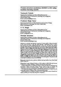
very difficult problems in probabilities and enumerative combinatorics [2, 8], regarding among other things the number of n−step SAW, their mean-square displacement, and the so-called scaling limit. The self-avoiding walks naturally appear in bioinformatics, during the prediction of the 3D conformation of a protein of interest. Frequently, the two dimensional backbone of the protein is looked for in a first stage, and then this 2D structure is refined step by step to obtain the final 3D conformation. Protein Structure Prediction (PSP) software can be separated into two categories. On the one hand, some algorithms construct the proteins’ structures on the 2D or 3D square lattice by adding, at each iteration, a new amino acid at the queue of the protein. Most of the time, various positions are possible for this amino acid, and the chosen position is the one that optimizes a given functional (for instance, the number of neighboring hydrophobic amino acids). On the other hand, some algorithms start from the straight line having the size of the considered protein, and they iterate pivot moves on this structure, pivot amino acids and angles being chosen to optimize another time a well-defined functional. We have pointed out, in our previous researches on the dynamics of the protein folding process [4, 5], that these two categories of protein structure prediction software cannot produce the same conformations [15]. More precisely, in the first category, all the conformations can be attained whereas it is not the case in the second one. Indeed this result, which is ignored by bioinformaticians, has been formerly discovered by the community of mathematicians that studies the self-avoiding walks (SAWs), even though the connection with the PSP problem has not been signaled. In their article introducing the pivot algorithm [23], Madras and Sokal have demonstrated a theorem showing that, when starting from the straight line of length n, and iterating the 180° rotation and either both 90° rotations or both diagonal reflections, all the n−step self-avoiding walks on Z2 can be obtained (or, in other words, their pivot algorithm is ergodic for this set of transformations). As a counterexample, they depicted in this article a 223-step SAW in Z2 that is not connected to any other SAW by 90° rotations (their counterexample is represented in Figure 1). This first apparition of an “unfolded” SAW was indeed the unique one in the literature, and the study of (un)folded SAWs has not been deepened before our work in [15]. In this article, the authors’ intention is to produce a list of first results and questionings about various sets of self-avoiding walks that can (or cannot) be attained by ±90° pivot moves, and to deduce consequences regarding the PSP software. After having recalled some basis on self-avoiding walks, we provide definitions of 4 subsets of SAWs that appear when considering such pivot moves, namely the folded SAWs obtained by iterating pivot moves on the straight line, the unfoldable SAWs, the set of SAWs that can be folded at least once, and finally the subset of self-avoiding walks that can be folded k times, k > 1. Then a list of results we have obtained on these subsets is provided. Among other things, the Cardinality of folded SAWs has been bounded, the infinite number of unfoldable SAWs is established (the proof of this result, too long to be presented in this article, is given in [6]), a shorter example of 2

unfoldable walk is given (107 steps), whereas the equality between the set of SAWs and the set of folded SAWs has been computationally verified until n 6 14. Relation between these subsets is then provided, before listing various open problems on (un)foldable self-avoiding walks. Theoretical aspects of this study are deepened in [6] whereas the computational ones are detailed in [7]. The remainder of this document is organized as follows. In the next section, a short overview about the self-avoiding walks is provided. This section enables us to introduce basic definitions and well-known results concerning these walks. Section 3 contains the rigorous definition of the subsets of self-avoiding walks regarded in this manuscript. Then, in Section 4, the first results we have obtained concerning the subset of unfolded SAW are detailed, whereas a non-exhaustive list of open questions is drawn up in Section 5. Consequences regarding the protein structure prediction problem are investigated in Section 6. This research work ends by a conclusion section, in which the contributions are summarized and intended future work is proposed.

2

A Short Overview of Self-Avoiding Walks

We firstly recall usual notations and well-known results regarding self-avoiding walks. We will bring partially, in a next section, these results in the folded SAWs subset.

2.1

Definitions and Terminologies

Let N be the set of all natural numbers, N∗ = {1, 2, . . .} the set of all positive integers, and for a, b ∈ N, a < b, the notation Ja, bK stands for the set {a, a + 1, . . . , b − 1, b}. |x| stands for the Euclidean norm of any vector x ∈ Zd , d > 1, whereas x1 , . . . , xd are the d coordinates of x. The n−th term of a sequence s is denoted by s(n). Finally, ]X is the Cardinality of a finite set X. Let us now introduce the notion of self-avoiding walk [19, 24, 27]. Definition 1 (Self-Avoiding Walk) Let d > 1. A n−step self-avoiding walk from x ∈ Zd to y ∈ Zd is a map w : J0, nK → Zd with: • w(0) = x and w(n) = y, • |w(i + 1) − w(i)| = 1, • ∀i, j ∈ J0, nK, i , j ⇒ w(i) , w( j) (self-avoiding property). Let d ∈ N∗ . Sn (x) is the set of n−step self-avoiding walks on Zd from 0 to x, cn (x) = ]Sn (x) is the Cardinality of this set, Sn = ∪x∈Zd Sn (x) is constituted P by all n−step self-avoiding walks that start from 0, whereas cn = x∈Zd cn (x) is the number of n−step self-avoiding walks on Zd starting from 0, that is, cn = ]Sn [27].

3

Figure 1: The first SAW shown to be not connected to any other SAW by 90° rotations (Madras and Sokal, [23]), that is, the first discovered unfoldable SAW.

2.2

Well-known results about self-avoiding walks

The objective of this section is not to realize a complete state of the art about established or conjectured results on SAWs, but only to present a few list of properties that are connected to our first investigations regarding the folded self-avoiding walks. For instance, the well-known pattern theorem [24] is not presented here. For further results about SAWs, readers can consult for instance [24, 27]. A first result concerning the number of n−step self-avoiding walks can be easily obtained by remarking that, when m−step SAWs are concatenated to n−step SAWs, we found all (m + n)−step self-avoiding walks and other walks having intersections. In other words, Proposition 1 ∀m, n ∈ N∗ , cm+n 6 cm cn . The existence of the so-called connective constant is a consequence of such a proposition. Theorem 1 The limit limn→∞ c1/n n exists. It is called the connective constant and is denoted by µ. Moreover, we have µn 6 cn and d 6 µ 6 2d − 1. Various bounds or estimates can be found in the literature [22, 27], like cn ≈ Aµn nγ−1 for A and γ to determine (predicted asymptotic behavior) and µ ∈ [2.625662, 2.679193]. The pivot algorithm is a dynamic Monte Carlo algorithm that produces selfavoiding walks using the following basic approach [23]. Firstly, a point p on the walk w is picked randomly and used as a pivot. Then a random symmetry operation of the lattice, like a rotation, is applied to the second part (suffixes) 4

of the walk, using p as origin. If the resulting walk is a SAW, it is accepted, else it is rejected and w is counted once again in the sample. A more detailed and precise algorithm can be found in [23]. In this article, it is shown that, quoting Madras and Sokal, Theorem 2 The pivot algorithm is ergodic for self-avoiding walks on Zd provided that all axis reflections, and either all 90° rotations or all diagonal reflections, are given nonzero probability. In fact, any N−step SAW can be transformed into a straight rod by some sequence of 2N − 1 or fewer such pivots. The pivot algorithm is ergodic too for SAWs on the square lattice [23], provided that the 180° rotation, and either both 90° rotations or both diagonal reflections, are given nonzero probability, whereas 90° rotations alone are not enough, due to Fig. 1.

3 3.1

Introducing the (un)folded self-avoiding walks Protein folding as preliminaries

Let us introduce the original context motivating the study of particular subsets of SAWs we called “folded” self-avoiding walks in the remainder of this document. In the 2 or 3 dimensional square lattice hydrophobic-hydrophilic model, simply denoted as HP model, which is used for low resolution backbone structure prediction of a given protein, hydrophobic interactions are supposed to dominate protein folding [4, 5]. This model was formerly introduced by Dill [13], who considers that the protein core freeing up energy is formed by hydrophobic amino acids, whereas hydrophilic amino acids tend to move in the outer surface due to their affinity with the solvent (see Fig. 2). In this model, a protein conformation is a SAW on a 2D or 3D lattice, depending on the level of resolution. This SAW is such that the free energy E of the protein, which depends on topological neighboring contacts between hydrophobic amino acids that are not contiguous in the primary structure, is minimal. In other words, for an amino acid sequence P of length n and for the set C(P) of all n−step SAWs, the walk chosen to represent the conformation of the protein is C∗ = min {E(C) | C ∈ C(P)} [26]. In that context and for a conformation (SAW) C, E(C) = −q where q is equal to the number of topological hydrophobic neighbors. For example, E(c) = −5 in Fig. 2. The overriding problem in PSP is: how to find such a minimal conformation, given all the n−step self-avoiding walks and the sequence of hydrophobicity of the protein ? To find the best 2D conformation of a protein, given its sequence of hydrophobicity, is really not an easy task. Indeed authors of [11] have proven that, considering the set of self-avoiding walks having n−steps and whose vertices are either black (hydrophobic) or white squares (hydrophylic residues), to determine the SAWs of this set that maximize the number of neighboring black 5

Figure 2: Hydrophilic-hydrophobic model (black squares are hydrophobic residues) squares is NP-hard. Given a sequence of amino acids, such statement leads to the use of heuristics to predict (and not to determine exactly) the most probable conformation of the protein. These heuristics operate as in the real biological world, folding or increasing the length of SAWs in order to minimize the free energy of the associated conformation: by doing so, the protein synthesis in aqueous environment is reproduced in silico. As stated previously, we have shown in a previous work that such investigations potentially lead to various subsets of self-avoiding walks [4, 5, 15]. In the first approach, starting from the straight line, we obtain by a succession of pivot moves of 90° a final conformation being a self-avoiding walk. In this approach, it is not regarded whether the intermediate walks are selfavoiding or not. Such a method corresponds to programs that start from the initial conformation, fold several times the linear protein, according to their embedded scoring functions, and then obtain a final conformation on which the SAW requirement is verified. It is easy to be convinced that, by doing so, the set of final conformations is exactly equal to the set of self-avoiding walks having n steps. As the conformations obtained by such methods coincide exactly to the well-studied global set of all SAWs, such an approach is not further investigated in what follows [15]. In the second approach, the same process is realized, except that all the intermediate conformations must be self-avoiding walks (see Fig. 3). The set of n−step SAWs reachable by such a procedure is denoted by f SAWn in what follows. Such a procedure is one of the two most usual translations of the socalled “SAW requirement” in the bioinformatics literature, leading to proteins’ conformations belonging into f SAWn . For instance, PSP methodes presented in [9, 16, 18, 20, 28] follow such an approach. We have shown in [15] that f SAWn ( Sn [23]. In other words, in this first category of PSP software, it is 6

Figure 3: Protein Structure Prediction by folding SAWs impossible to reach all the conformations of Sn . Other approaches in the same category can be imagined, like the following one. We can act as above, requiring additionally that no intersection of vertex or edge during the transformation of one SAW to another occurs. For instance, the pivot move of Figure 4 is authorized in the previous f SAW approach, but it is refused in the current one: during the rotation around the residue having a cross, the rigid structure after this residue intersects the remainder of the “protein” (see Fig. 5). In this two dimensional approach denoted by f SAW 0 , it is impossible for a protein folding from one plane conformation to another plane one to use the 3D space to achieve this folding. A reasonable modeling of the true natural folding dynamics of an already synthesized protein can be obtained by extending this requirement to the third dimension. However, due to its complexity, this requirement is actually never used by tools that embed a 2D HP square lattice model for protein structure prediction. This is why these particular SAWs are not really investigated in this document. Let us just emphasize that f SAWn0 is obviously a subset of f SAWn , but there is a priori no reason to consider them equal. Indeed, Figure 6 shows that, Proposition 2 For all n ∈ N∗ , f SAWn0 ⊂ f SAWn . However, ∃n ∈ N∗ , f SAWn0 , f SAWn . Proof In Figure 6, the unique possible pivot move is the red dot, and obviously such move leads to the intersection between the head and the queue of the 7

Figure 4: Pivot move acceptable in f SAW but not in f SAW 0

Figure 5: An intersection appears between the head and the queue during the transformation, thus this pivot move is refused in f SAW 0 . structure during the transformation. Note that we only studied pivot moves of ±90° in the three previous approaches. But to consider other sets of transformations could be interesting in some well-defined contexts, which can potentially lead to different new subsets of SAWs. A last bioinformatics approach of protein structure prediction using selfavoiding walks starts with an 1−step SAW, and at iteration k, a new step is added at the queue of the walk, in such a way that the new k−step selfavoiding walk presents the best value for the considered scoring function (see Fig 7). The protein is thus constructed step by step, reaching the best local conformation at each iteration. It is easy to see that such an approach leads, another time, to all the possible self-avoiding walks having the length of the 8

Figure 6: f SAWn , f SAWn0 considered protein [15]. In the remainder of this document, we give a more rigorous definition of the f SAWn set, we initiate its study, and compare it to the well-known Sn SAWs set.

3.2

Notations

Folded self-avoiding walks can be studied in a lattice having d dimensions. However, for the sake of simplicity, authors of this research work have decided to introduce them only on the 2 dimensional square lattice Z2 , to be as closed as possible to their field of application: the low resolution backbone structure prediction of a protein. Such restriction enables us to produce understandable pictures of such not yet investigated particular walks. One of the easiest way to define the folded self-avoiding walks described previously, that appear during the realization of the SAW requirement in PSP algorithms, is to introduce the absolute encoding of a walk [3, 17]. In this  n+1 with w(0) = (0, 0) is a encoding, a n + 1−step walk w = w(0), . . . , w(n) ∈ Z2 sequence s = s(0), . . . , s(n − 1) of elements belonging into Z/4Z, such that: • s(i) = 0 if and only if w(i + 1)1 = w(i)1 + 1 and w(i + 1)2 = w(i)2 , that is, w(i + 1) is at the East of w(i). • s(i) = 1 if and only if w(i + 1)1 = w(i)1 and w(i + 1)2 = w(i)2 − 1: w(i + 1) is at the South of w(i). • s(i) = 2 if and only if w(i + 1)1 = w(i)1 − 1 and w(i + 1)2 = w(i)2 , meaning that w(i + 1) is at the West of w(i). • Finally, s(i) = 3 if and only if w(i + 1)1 = w(i)1 and w(i + 1)2 = w(i)2 + 1 (w(i + 1) is at the North of w(i)). Let us now define the following functions [15]. 9

Figure 7: Protein Structure Prediction by stretching SAWs Definition 2 The anticlockwise fold function is the function f : Z/4Z −→ Z/4Z defined by f (x) = x − 1 (mod 4) and the clockwise fold function is f −1 (x) = x + 1 (mod 4). Using the absolute encoding sequence s of a n−step SAW w that starts from the origin of the square lattice, a pivot move of +90° on w(k), k < n, simply consists to transform s into s(0), . . . , s(k − 1), f (s(k)), . . . , f (s(n)). Similarly, a pivot move of −90° consists to apply f −1 to the queue of the absolute encoding sequence, like in Figure 8.

3.3

A graph structure for SAWs folding process

We can now introduce a graph structure describing well the iterations of ±90° pivot moves on a given self-avoiding walk. Given n ∈ N∗ , the graph Gn , formerly introduced in [15], is defined as follows: • its vertices are the n−step self-avoiding walks, described in absolute encoding; • there is an edge between two vertices si , s j if and only if s j can be obtained by one pivot move of ±90° on si , that is, if there exists k ∈ J0, n − 1K s.t.: 10

(b) 001222 = 00 f −1 (0) f −1 (1) f −1 (1) f −1 (1)

(a) 000111

Figure 8: Effects of the clockwise fold function applied on the four last components of an absolute encoding. – either si (0), . . . , si (k − 1), f (si (k)), . . . , f (si (n)) = s j – or si (0), . . . , si (k − 1), f −1 (si (k)), . . . , f −1 (si (n)) = s j . Such a digraph is depicted in Figure 9. The circled vertex is the straight line whereas strikeout vertices are walks that are not self-avoiding. Depending on the context, and for the sake of simplicity, Gn will also refer to the set of SAWs in Gn (i.e., its vertices). Using this graph, the folded SAWs introduced in the previous section can be redefined more rigorously. Definition 3 f SAWn is the connected component of the straight line 00 . . . 0 (n times) in Gn , whereas Sn is constituted by all the vertices of Gn . The Figure 1 shows that the connected component f SAW(223) of the straight line in G223 is not equal to the whole graph: G223 is not connected. More precisely, this graph has a connected component of size 1: Figure 1 is totally unfoldable, whereas SAW of Fig. 6 can be folded exactly once. Indeed, to be in the same connected component is an equivalence relation Rn on Gn , ∀n ∈ N∗ , and two SAWs w, w0 are considered equivalent (with respect to this equivalence relation) if and only if there is a way to fold w into w0 such that all the intermediate walks are self-avoiding. When existing, such a way is not necessarily unique. These remarks lead to the following definitions. Definition 4 Let n ∈ N∗ and w ∈ Sn . We say that: • w is unfoldable if its equivalence class, with respect to Rn , is of size 1; • w is a folded self-avoiding walk if its equivalence class contains the n−step straight walk 000 . . . 0 (n − 1 times); • w can be folded k times if a simple path of length k exists between w and another vertex in the same connected component of w. Moreover, we introduce the following sets: 11

• f SAW(n) is the equivalence class of the n−step straight walk, or the set of all folded SAWs. • f SAW(n, k) is the set of equivalence classes of size k in (Gn , Rn ). • USAW(n) is the set of equivalence classes of size 1 (Gn , Rn ), that is, the set of unfoldable walks. • f 1 SAW(n) is the complement of USAW(n) in Gn . This is the set of SAWs on which we can apply at least one pivot move of ±90. Example 1 Figure 10 shows the two elements of a class belonging into f SAW(219, 2) whereas Fig. 1 is an element of USAW(223).

4

A Short List of Results on (un)folded Self-Avoiding Walks

We now give a first collection of easy-to-obtained results concerning the particular SAW sets introduced in the previous section. These results have been either obtained mathematically or by using computers. We firstly show that, Proposition 3 The cardinality φn of f SAWn satisfies: 2n+2 6 φn 6 4 × 3n . This result is a consequence of the following lemma. Lemma 1 The 2n n−step walks that take steps only in the positive coordinate directions are in f SAW(n). This lemma can be proven using the number of cranks of a self-avoiding walk, defined below. Definition 5 (Crank) Let w be a n−step self-avoiding walk on Z2 of absolute encoding s. w contains a crank at position k ∈ J1, nK if s(k − 1) , s(k).

Proof (Lemma 1) Let n ∈ N∗ . We show by a mathematical induction that, ∀N ∈ N, any n−step self-avoiding walk that (1) takes steps only in the positive coordinate directions, and (2) has N cranks, is in f SAW(n). The base case is obvious, as if N = 0, then w is a straight line. Let N ∈ N such that the statement holds for all k 6 N, and consider a n−step self-avoiding walk w that has N + 1 cranks while taking steps only in the positive coordinate directions. Let j be the position of the first crank in w. As steps are taken only in the positive coordinate directions, only two situations can occur (see Figure 11): (1) w( j) = w(j − 1) + (1, 0) and w( j + 1) = w( j) + (0, 1) (s( j − 1) = 0, s(j) = 3), or (2) w(j) = w(j − 1) + (0, 1) and w( j + 1) = w( j) + (1, 0) (s( j − 1) = 3, s( j) = 0). Suppose now that the origin of the 2D square lattice is set to w( j). So, in the first situation (1), 12

Figure 9: The digraph G3 = f SAW(3)

13

Figure 10: The two self-avoiding walks in f SAW(219, 2) • ∀l > j, w(l) = (w(l)1 , w(l)2 ) is such that w(l)1 > 0 while w(l)2 > 1, • ∀l < j, w(l) = (w(l)1 , w(l)2 ) is such that w(l)1 6 −1 while w(l)2 6 0. The effect of a 90 pivot move on the origin w( j) is to reduce the number of cranks N + 1 to N in w, and to map each w(l) = (w(l)1 , w(l)2 ) into (w(l)2 , w(l)1 ), ∀l > j. After such a pivot move, the obtained walk w0 is such that ∀l > j, w0 (l)1 = w(l)2 > 1, while ∀l < j, w0 (l)1 = w(l)1 6 −1. In other words, the walk w0 still remains self-avoiding. w0 having N cranks, it belongs into f SAW(n) due to the induction hypothesis. Furthermore, w0 is obtained by operating a pivot move on w, thus these two walks belong into the same connective component of Gn . Finally, w ∈ f SAW(n). The second situation (2) also can be handled in that way, which concludes the mathematical induction and the proof of the lemma. Proof (Proposition 3) Due to Lemma 1, we have φn > 4 × 2n (4× because of the 4 quarters of the square lattice). And since the set of n−step walks without immediate reversals has cardinality 4 × 3n and contains all n−step folded selfavoiding walks, we have φn 6 4 × 3n . Remark 1 In particular, SAWs whose absolute encoding is only constituted by 0’s and 1’s are folded SAWs. It is quite possible that a few 2’s or 3’s can be added without breaking the folded character of the walk, meaning that the lower bound could be increased. We can now give a result regarding the USAW(n) set of self-avoiding walks. Theorem 3 There is an infinite number of n such that USAW(n) is nonempty. In particular, the number of unfoldable SAWs is infinite. Proof A proof of this result, too long to be contained in this work, can be found in [6]. It consists to create a recursive construction process of unfoldable self-avoiding walks, as depicted in Figure 17. 14

Figure 11: Walks that contain only 3 and 0 in their absolute encoding are folded SAWs: reducing the number of cranks does not introduce intersections in the walk. Proposition 4 ∀n 6 14, f SAW(n) = Gn whereas f SAW(107) ( G107 (see Figure 13). In other words, let νn the smallest n > 2 such that USAW(n) , ∅. Then 15 6 νn 6 107. Proof We have computed a program that constructs the connected component of the n−step straight line for n 6 14, and at each time, we have obtained the whole Gn (see [7]). Additionally, we have obtained using a backtracking method the walk depicted in Figure 14, which justifies the upper bound of 107: we have verified using a systematic program that no pivot move can be realized in that walk without breaking the self-avoiding requirement. These programs, their explanations and justifications can be found in [7]. Proposition 5 ∀n 6 28, f 1 SAW(n) = Gn . Proof Obtained experimentally, see [7]. The results contained into the two previous propositions are summarized, with all intermediate computations, in Table 1. The ]Gn values, obtained in [21], are recalled here for comparison. Until now, connected components presented in this paper either have the straight line, or are of size 1 or 2. A reasonable questioning is to wonder whether it is possible to have larger connected components different from the one of the straight line. We are founded to claim that, Proposition 6 It exists k > 2 such that f SAW(n, k) is nonempty. In other words, connected components different from f SAW(n) and larger than 1 or 2 elements exist. The result, which has been experimentally obtained, 15

n 1 2 3 4 5 6 7 8 9 10 11 12 13 14 15 16 17 18 19 20 21 22 23 24 25 26 27 28 29 30 31 .. .

]Gn 4 12 36 100 284 780 2172 5916 16268 44100 120292 324932 881500 2374444 6416596 17245332 46466676 124658732 335116620 897697164 2408806028 6444560484 17266613812 46146397316 123481354908 329712786220 881317491628 2351378582244 6279396229332 16741957935348 44673816630956 .. .

] f 1 SAW(n) 4 12 36 100 284 780 2172 5916 16268 44100 120292 324932 881500 2374444 6416596 17245332 46466676 124658732 335116620 897697164 2408806028 6444560484 17266613812 46146397316 123481354908 329712786220 881317491628 2351378582244 ? ? ? .. .

]USAW(n) = ] f 1 SAW(n) 0 0 0 0 0 0 0 0 0 0 0 0 0 0 0 0 0 0 0 0 0 0 0 0 0 0 0 0 ? ? ? .. .

] f SAW(n) 4 12 36 100 284 780 2172 5916 16268 44100 120292 324932 881500 2374444 ? ? ? ? ? ? ? ? ? ? ? ? ? ? ? ? ? .. .

107

?

?

>1

?

Table 1: Cardinalities of various subsets of SAWs

16

(a) w0 (239-step walk)

(b) w1 (391-step walk)

(c) w2 (575-step walk)

(d) w3 (791-step walk)

Figure 12: Generating walks that cannot be folded out can be proven by exhibiting a counterexample: Figure 15 shows a connected component of size 5. We can define a diameter function D on the connected components of Gn , such that D(C) is the length of the longest shortest path in the connected component C of Gn . Consider the connected component of the straight line f SAW(n), we have the result, Proposition 7 The diameter of f SAW(n) is equal to 2n: D( f SAW(n)) = 2n. Proof We take the SAW Sz1 defined as the zigzag (0, 1, 0, 1, 0, ...) and the Sz2 defined as the zigzag (2, 1, 2, 1, 2, ...). We can transform Sz1 in (2, 3, 2, 3, 2, ...) by two pivot moves: (0, 1, 0, 1...) → (1, 2, 1, 2, 1, ...) → (2, 3, 2, 3, 2, ...).

17

f1SAW(n)

fSAW(n)

nfSAW(n)

fSAW(n) = f1SAW(n)

(a) Gn for n 6 14

(b) Diagram of Gn for n = 107

Figure 13: Vien diagram for Gn

Figure 14: Current smallest (107-step) SAW that cannot be folded out

Figure 15: A connected component with 5 elements

18

Figure 16: The digraph G2 = f SAW(2) Then two other pivot moves allow us to transform (2, 3, 2, 3, 2, ...) in (2, 1, 0, 1, 0, ...), that is, (2, 3, 2, 3, 2, ...) → (2, 2, 1, 2, 1, 2, ...) → (2, 1, 0, 1, 0, 1, ...). As the respective visited vectices start by (0, 1), (1, 2), (2, 3), (2, 2), (2, 1), we obtain by doing so a simple path of length 4. The process can be reproduced on the queue (0, 1, 0...) of (2, 1, 0, 1, 0...) until each 0’s (odd positions) of the SAW has been transformed to 2, and each 1’s (even position) has been set again to 1. As there are two pivot moves for each value in the path and each pivot moves is in a different direction in Gn , so the minimum distance from Sz1 to Sz2 in Gn is 2n. This path, from Sz1 to Sz2 , is the largest distance we can find in Gn as we have two pivot moves on each edge. If we add indeed one more pivot move, i.e., three pivot moves, on an edge then the same value could be obtained from the initial position by making only one pivot move in the opposite direction which would reduce the distance between the two SAWs. Example 2 In f SAW(2), this diameter corresponds, for instance, to the shortest path 03 → 00 → 11 → 12 → 23 (see Figure 16).

19

5

A list of Open Questions

We enumerate in this section a list of open questions that have appeared to us as interesting. Some of them should be very easy to solve, whereas other ones may involve a degree of difficulty. In the following we define f SAW d (n) as the class of equivalency of the n−step straight walk on Zd and Gdn is the equivalent of Gn in Zd . Note that f SAW 2 (n) is equal to f SAW(n), as introduced in Definition 3.3. 1. For any dimension d, do we have the existence of n ∈ N∗ such that f SAW d (n) ( Gdn ? 2. f SAW 2 (2) and f SAW 2 (3) are obviously connected graphs, but they are not Eulerian. Indeed, more than two vertices have an odd degree both in f SAW 2 (2) and f SAW 2 (3) (see Figures 16 and 9). Is it the case for all f SAW d (n) ? 3. f SAW 2 (2) and f SAW 2 (3) are Hamiltonian graphs, with the following Hamiltonian circuits: • 00 → 03 → 32 → 23 → 10 → 11 → 22 → 33 → 30 → 21 → 12 → 01 → 00 for f SAW 2 (2) (see Figure 16). • 000 → 003 → 010 → 011 → 012 → 001 → 030 301 → 300 → 333 → 322 → 321 → 332 → 303 230 → 223 → 212 → 211 → 210 → 221 → 222 121 → 122 → 123 → 112 → 101 → 100 → 103 → for f SAW 2 (3) (see Figure 9).

→ 323 → 330 → → 232 → 233 → → 111 → 110 → 032 → 033 → 000

Is it a coincidence, or is it the case for every f SAW d (n) ? 4. What is the exact value of the diameter D( f SAW d (n)) ? 5. Do we have a connective constant for f SAW d (n). That is, does the limit limn→+∞ φ1/n n exist, and can we bound it ? 6. un = ]USAW d (n) is an increasing sequence (for d = 2, or for any d)? Does it grow at a given (linear or exponential) rate? 7. Let k ∈ N. Is the sequence vn = ] f SAW(n, k) increasing with n ? If so, at which rate, and does it depend on the dimension d? And what about the sequence wk = ] f SAW(n, k) for a given n ? 8. More simply, is there an unfoldable walk in Z3 ? 9. Are the connected components of Gdn convex ? In other words, given two SAWs in a same component C. Are all (or at least one) the shortest paths connecting them on Zd in C?

20

10. Is there a generating function expressing the folded self-avoiding walks more simply, making it possible to enumerate them on the square lattice (like what has been realized in [10]). 11. When we can fold a self-avoiding walk until a straight line, is it possible to fold it in such a way that the number of cranks decreases ? And for two given self-avoiding walks wi and w j of the same connected component of Gn , such that wi has more cranks than w j , is there a path from wi to w j whose vertices’ number of cranks is decreasing ? Is there a relation between the vertex depth and the number of cranks in Zd ?

6

Consequences on Protein Folding

This first theoretical study about folded self-avoiding walks raises several questions regarding the protein structure prediction problem and the current ways to solve it. In one category of PSP software, the protein is supposed to be synthesized first as a straight line of amino acids, and then this line of a.a. is folded out until reaching a conformation that optimizes a given scoring function. By doing so, the obtained backbone structures all belong into f SAW(n), where n is the number of residues of the protein. The second category of PSP software consider that, as the protein is already in the aqueous solvent, it does not wait the end of the synthesis to take its 3D conformation. So they consider SAWs whose number of steps increases from 1 to the number of amino acids of the targeted protein and, at each step k, the current walk is streched (one amino acid is added to the protein) in such a way that the pivot k is placed in the position that optimizes the scoring function they consider. By doing so, the possible predicted backbones are the whole G3 . The two sets of possible conformations are different, at least when considering 2D low resolution models. We show by this work that (1) to take place in the first situation (folding the straight line by a succession of pivot moves) can be interesting as the number of possible SAW conformations is smaller than ]Gn . Indeed this interest is ] f SAW(n) directly related to the rate < 1. If this rate decreases dramatically ]Gn when n increases, then the computational advantage is obvious. However,we have currently no idea of such a gain, that is, of the growing rate of ] f SAW(n) compared to ]Gn < 1. (2) The use of heuristics instead of exact methods (like SAT solvers for instance) is a priori not justified for PSP software that fold the straight line. Indeed, the PSP problem has been proven NP hard on the set Gn of all possible SaWs. As they consider a strict subset of it, the complexity of the problem might be reduced due to a lower number of cases to consider. However, Proposition 3 tends to indicate that this problem still remains difficult in f SAW(n), which nevertheless necessitates a rigorous complexity proof. (3) Biologically speaking, to suppose that the proteins wait to be completely synthesized before starting to fold appears as unrealistic, as the synthesis occurs in an aqueous solvent. Indeed, the protein starts to fold during 21

(a) Conformation having best score (27)

(b) Second best conformation (score 24)

Figure 17: Illustration of chaos in protein folding (conformations have been predicted using RaptorX) its synthesis. Furthermore, to the authors’ opinion, it is restrictive to consider that the head of the protein definitively stops to fold after having synthesized. Such a supposition is equivalent to make a confusion between local (the SAW at step k) and global (the final optimal SAW) optimization. Indeed, authors of this manuscript recognize honestly that they have no idea to determine if this third approach (continuously folding the walk while stretching it) is more reasonable than the previous ones, and if it is equivalent to either f SAW(n) or 22

to Gn (or if it constitutes a third different subset of SAWs). The authors’ goal is only to point out the importance to determine the best dynamical system to model protein folding before programming it in PSP software, as this model determine which conformations can be predicted. A last remark to emphasize the importance of such a study: authors of [4] have proven that the dynamical system used in the “folding the straight line” category is chaotic according to Devaney, meaning that any wrong choice of pivot move (due to approximations in the scoring function, for instance) can potentially become dramatic. Other researches ( [9] for instance) tend to show that the protein folding process intrinsically embeds a certain amount of chaos. Thus, to use a more or less erroneous model to predict the conformation could have grave consequences in prediction quality. Figure 17 shows the two best conformations predicted by RaptorX [25], a well-known PSP software. We can see that using twice a same model, but with different parameters can potentially lead to quite different conformations, illustrating a possible effect of some chaotic properties exhibited by the chosen model. We can reasonably wonder what is the effect of a wrong model in such a prediction.

7

Conclusion

In this paper, the problem of self-avoiding walks folding in the square lattice has been tackled. Regarding the protein structure prediction problem, we have shown that the set of generated self-avoiding walks depends on the PSP software category. In particular some particular conformations cannot be reached by just folding the straight line whereas they can be generated using random SAW generators as the pivot algorithm. Starting from this fact, we have proposed a further exploration of the folded self-avoiding walks. Different subsets of self-avoiding walks have been defined, like the set of unfoldable walks. We have shown that, even though their is an infinite number of unfoldable SAWs, the number of folded SAWs is still exponential. After having described the first obtained results on (un)folded SAWs, we have proposed a list of open questions that could be explored on these SAWs. Lastly, the link between (un)folded SAWs and proteins has been questioned, and the consequences of the PSP software choice on protein conformation has been highlighted. Several research problems are interesting to further study and better understand the properties of (un)folded SAWs, as shown in the open questions section. Our future work will be concentrated on finding the smallest unfolded SAWs, finding the smallest connected components of unfolded SAWs, and on the optimization of energy levels of a given folded SAW.

8

Acknowledgement

The authors wish to thank Kamel Mazouzi, Thibaut Cholley, Raphaël Couturier, and Alain Giorgetti for their help in understanding USAWs. All the compu-

23

tations presented in the paper have been performed on the supercomputer facilities of the Mésocentre de calcul de Franche-Comté.

References [1] Proceedings of the IEEE Congress on Evolutionary Computation, CEC 2010, Barcelona, Spain, 18-23 July 2010. IEEE, 2010. [2] Axel Bacher and Mireille Bousquet-Mélou. Weakly directed self-avoiding walks. J. Comb. Theory Ser. A, 118(8):2365–2391, November 2011. [3] R. Backofen, S. Will, and P. Clote. Algorithmic approach to quantifying the hydrophobic force contribution in protein folding, 1999. [4] Jacques Bahi, Nathalie Côté, and Christophe Guyeux. Chaos of protein folding. In IJCNN 2011, Int. Joint Conf. on Neural Networks, pages 1948–1954, San Jose, California, United States, July 2011. [5] Jacques Bahi, Nathalie Côté, Christophe Guyeux, and Michel Salomon. Protein folding in the 2D hydrophobic-hydrophilic (HP) square lattice model is chaotic. Cognitive Computation, 4(1):98–114, 2012. [6] Jacques M. Bahi, Alain Giorgetti, and Christophe Guyeux. Unfoldable self-avoiding walks are infinite. Consequences for the protein structure prediction problem. arXiv.org, 2013. [7] Jacques M. Bahi, Christophe Guyeux, Kamel Mazouzi, and Laurent Philippe. Computational investigations of folded self-avoiding walks related to protein folding. arXiv.org, 2013. [8] Nicholas R. Beaton, Philippe Flajolet, Timothy M. Garoni, and Anthony J. Guttmann. Some new self-avoiding walk and polygon models. Fundam. Inf., 117(1-4):19–33, January 2012. [9] Michael Braxenthaler, R. Ron Unger, Ditza Auerbach, and John Moult. Chaos in protein dynamics. Proteins-structure Function and Bioinformatics, 29:417–425, 1997. [10] A. R. Conway, I. G. Enting, and A. J. Guttmann. Algebraic techniques for enumerating self-avoiding walks on the square lattice. Journal of Physics A Mathematical General, 26:1519–1534, April 1993. [11] Pierluigi Crescenzi, Deborah Goldman, Christos Papadimitriou, Antonio Piccolboni, and Mihalis Yannakakis. On the complexity of protein folding (extended abstract). In Proceedings of the thirtieth annual ACM symposium on Theory of computing, STOC ’98, pages 597–603, New York, NY, USA, 1998. ACM.

24

[12] P. G. de Gennes. Exponents for the excluded volume problem as derived by the Wilson method. Physics Letters A, 38(5):339–340, February 1972. [13] KA Dill. Theory for the folding and stability of globular proteins. Biochemistry, 24(6):1501–9–, March 1985. [14] Paul J. Flory. The Configuration of Real Polymer Chains. The Journal of Chemical Physics, 17(3):303–310, 1949. [15] Christophe Guyeux, Bahi Jacques M., Côté Nathalie, and Bienia Wojciech. Is protein folding problem really a NP-complete one ? First investigations. Soumis à Journal of Bioinformatics and Computational Biology (Elsevier), October 2012. [16] Trent Higgs, Bela Stantic, Tamjidul Hoque, and Abdul Sattar. Genetic algorithm feature-based resampling for protein structure prediction. In IEEE Congress on Evolutionary Computation [1], pages 1–8. [17] Md. Hoque, Madhu Chetty, and Abdul Sattar. Genetic algorithm in ab initio protein structure prediction using low resolution model: A review. In Amandeep Sidhu and Tharam Dillon, editors, Biomedical Data and Applications, volume 224 of Studies in Computational Intelligence, pages 317–342. Springer Berlin Heidelberg, 2009. [18] Dragos Horvath and Camelia Chira. Simplified chain folding models as metaheuristic benchmark for tuning real protein folding algorithms? In IEEE Congress on Evolutionary Computation [1], pages 1–8. [19] Barry D. Hughes. Random walks and random environments, Volume 1: Random walks. Clarendon Press, Oxford, March 1995. [20] Md. Kamrul Islam and Madhu Chetty. Clustered memetic algorithm for protein structure prediction. In IEEE Congress on Evolutionary Computation [1], pages 1–8. [21] Iwan Jensen. Enumeration of self-avoiding walks on the square lattice. J. Phys. A, pages 5503–5524, 2004. [22] Iwan Jensen. Improved lower bounds on the connective constants for two-dimensional self-avoiding walks. Journal of Physics A: Mathematical and General, 37(48):11521+, 2004. [23] Neal Madras and Alan D. Sokal. The pivot algorithm: A highly efficient monte carlo method for the self-avoiding walk. Journal of Statistical Physics, 50:109–186, 1988. [24] Neal Noah Madras and Gordon Slade. The self-avoiding walk. Probability and its applications. Birkhäuser, Boston, 1993. [25] Jian Peng and Jinbo Xu. Raptorx: Exploiting structure information for protein alignment by statistical inference. Proteins, 79(S10):161–171, 2011. 25

[26] Alena Shmygelska and Holger Hoos. An ant colony optimisation algorithm for the 2d and 3d hydrophobic polar protein folding problem. BMC Bioinformatics, 6(1):30, 2005. [27] Gordon Slade. The self-avoiding walk: a brief survey. Blath, Jochen (ed.) et al., Surveys in stochastic processes. Selected papers based on the presentations at the 33rd conference on stochastic processes and their applications, Berlin, Germany, July 27–31, 2009. Zürich: European Mathematical Society (EMS). EMS Series of Congress Reports, 181-199 (2011)., 2011. [28] Ron Unger and John Moult. Genetic algorithm for 3d protein folding simulations. In Proceedings of the 5th International Conference on Genetic Algorithms, pages 581–588, San Francisco, CA, USA, 1993. Morgan Kaufmann Publishers Inc.

26