of a number of distinct image feature points are used to compute the motions and relative ... In this approach the image motion is represented by an image velocity field ..... equations in seven unknowns). ..... maximum error in the solution can be estimated in all cases given the ... (All values are rounded to the sixth decimal.
.ps11 INTERPRETATION OF IMAGE FLOW: A SPATIO-TEMPORAL APPROACH
Muralidhara Subbarao Abstract Research on the interpretation of image flow (or optical flow) until now has mainly focused on instantaneous flow fields. This limits the scope of the problems that one can address and the accuracy of the results. Here we extend a previous formulation of the problem to incorporate temporal variation of image flow. We illustrate our approach by solving specific cases which are of practical significance including simple cases of non-rigid and non-uniform motions. The formulation is general in that it is applicable to any situation provided that the scene geometry, the scene transformation, and the image flow are all ‘‘smooth’’ or analytic. For the case of rigid and uniform motion we have obtained some results which are of practical value. We have shown that only the first-order spatial and temporal derivatives of image flow are sufficient to recover the local surface orientation and motion; second-order (or higher order) derivatives whose measurement is unreliable are not necessary. (In comparison, previous methods use up to second-order spatial derivatives.). Further, the representation and the solution method used here have some advantages in comparison with the existing approaches; they facilitate a uniform approach to all cases of rigid motion (including the case of interpreting instantaneous visual motion).
Index Terms - Three-dimensional interpretation of image flow, optical flow, motion analysis, surface structure and transformation recovery.
1
I. Introduction The motion of an object relative to a camera produces a moving image on the camera’s image plane. The image motion thus produced contains valuable information about the threedimensional (3D) shape and motion of the object. Recovering this 3D information from image motion is the topic of this paper. The approaches that have been taken in solving this problem fall under two major categories, discrete and continuous. In the discrete approach, the velocities of a number of distinct image feature points are used to compute the motions and relative positions of the corresponding points in the scene. (e.g.: [8,27,16,25,26]). In this paper we take the continuous approach. In this approach the image motion is represented by an image velocity field or image flow. Image flow is a two-dimensional velocity field defined over the camera’s image plane. The velocity at any point is the instantaneous velocity of the image element at that point. Some authors refer to image flow as optical flow. Methods for the computation of image flow from time-varying intensity images have been proposed by many researchers (e.g.: [7,10,9,32,35]). This paper is concerned with the interpretation of image flow, i.e. recovering the geometry and the motion of objects in a scene from their image flow. Here we assume that the image flow is given. Methods for interpreting instantaneous image flow have been proposed by many researchers (e.g.: [13,15,17,11,23,30,20]). However, previous work on using temporal variation of image flow is scarce. Use of temporal information is necessary for two reasons. First, in many cases we can trade noise-sensitive spatial information for relatively robust temporal information. Ullman [28], in his work that belongs to the discrete category of approaches mentioned earlier, has the following to say: ‘‘.... although the instantaneous velocity field contains sufficient information for the recovery of the 3-D shape, the reliable interpretation of local structure from motion requires the integration of information over a more extended time period.’’ This remark holds equally well for the continuous approach. For example, consider a small surface patch in motion which is approximately planar. For this case we show here that, in general, we can use the first order temporal derivatives of image flow in place of the second-order spatial derivatives. The measured values of second-order derivatives are usually very unreliable in comparison with the first-order derivatives. Therefore using temporal derivatives is preferable in this case. 2
The second and more important reason for using temporal information is that it makes possible for us to deal with more complicated situations such as when the object in view is undergoing non-uniform (or accelerated) motion and non-rigid motion. In the domain of continuous approaches there has been very little research on this topic. In this paper we present a general formulation capable of handling arbitrarily complicated cases under a ‘‘smoothness’’ assumption. This assumption states that the scene geometry, scene transformation (i.e. motion and deformation), and image flow are all locally ‘‘smooth’’. Recently Bandopadhyay and Aloimonos [4] and Wohn and Wu [36] have used temporal information to solve a restricted case of rigid motion. This case is the one we have considered in Section IV.B.1.a. A systematic way of incorporating temporal information in the interpretation of image flow was proposed in [21]. This paper is is mainly based on this work.
II. Summary of results A major portion of this paper is devoted to the study of image flow resulting from rigid motion of objects. Here the problem is to determine the three-dimensional shape and rigid motion of surfaces from their image flow. In this paper, equations relating the local orientation and motion of a surface and the first order spatio-temporal image flow derivatives are derived. These equations are solved to obtain the orientation and motion in closed form. Also, an interesting case where a camera tracks a point on a moving surface is solved with the knowledge of the camera’s tracking motion. Then this formulation is extended to deal with non-uniform or accelerated motions. This extension is illustrated with a simple example. Finally the formulation for rigid motion is generalized to deal with non-rigid motion. This again is illustrated with a simple example. This general formulation leads to some new insights into the intrinsic nature of the image flow interpretation problem. It makes explicit the well known fact that the image flow interpretation in a general case is inherently underconstrained and that additional assumptions about the scene are necessary to solve the problem. It gives the minimum number of additional constraints (in the form of assumptions about the scene) necessary to solve the problem. For example, it exposes the fact that the rigidity assumption, the assumption that objects in the scene are rigid, is a sufficient constraint. 3
In this paper we have not included any specific case which involves second or higher order image flow parameters. Two such cases dealing with the interpretation of instantaneous image flow for planar and curved surfaces can be found in [22]. Since these two cases have received a great deal of attention in the past, we mention here that we have obtained closed form solutions to both planar and curved surfaces using the theoretical framework described here. Also, we have been able to prove many results concerning the multiplicity of interpretations for these cases. Theoretically the framework described here can deal with cases involving higher order image flow parameters, but their practical importance is not clear.
III. Strategy of formulation and analysis We restrict the image flow analysis to be local, both in space and in time. This restriction helps to keep the number of parameters small and makes the analysis tractable. Further, in a small field of view and over a short period of time, the following are assumed to be ‘‘smooth’’ and changing slowly (i) the shape of the visible surface patch, (ii) the transformation (or motion and deformation) of the surface patch with time, and (iii) the image flow. A local analysis such as this must be preceded by a detection of discontinuities in the image flow field corresponding to discontinuities in the geometry and the transformation of surfaces in the scene. This problem has been addressed by several researchers (e.g.: [9,1,24,34,33,35]). Having located such discontinuities in the motion field a local analysis is carried out in small image regions not containing these discontinuities to recover the structure and motion of the corresponding surfaces in the scene. A patching together of this local three-dimensional information is necessary to obtain a global description of the scene.
IV. Rigid motion case First we consider three cases where the motion is rigid and uniform and one more case where the motion is non-uniform. The three rigid motion cases considered here cover a large class of problems of practical interest. Of the three rigid uniform motion cases, the first two relate to the case where the image flow is observed in a fixed image neighborhood and the third relates to the case where the camera tracks a point on the object in motion and the tracking 4
motion of the camera is known. In all three cases we have solved for the local orientation and rigid motion of the surface patch.
A. Formulation A pin-hole camera with a spherical projection screen whose center is at the pin-hole or the focus is a good camera model. For this camera model, due to symmetry, the image flow analysis is identical at all regions on the projection screen. However, actual camera systems usually have a planar screen. We adopt this planar projection screen model in our analysis. The geometry of the screen is entirely a matter of convenience and does not affect our results. Note that there is a one to one correspondence between an image on a curved screen such as a spherical screen and an image on a planar screen. The choice of the planar screen geometry restricts our analysis to the field of view along the optical axis. However, the image flow in a field of view not along the optical axis can be analyzed by first projecting the image velocities on to a plane perpendicular to the field of view. (In this case, if the plane is at unit distance in front of the focus then the same analysis in this paper holds.) This projection process is quite straightforward [12].
******** FIGURE 1 ABOUT HERE *********
The camera model is illustrated in Figure 1. The origin of a Cartesian coordinate system OXYZ forms the focus and the Z-axis is aligned with the optical axis. The image plane is assumed to be at unit distance from the origin perpendicular to the optical axis. The image coordinate system oxy on the image plane has its origin at (0,0,1) and is aligned such that the x and y axes are, respectively, parallel to the X and Y axes. The entire coordinate system is fixed with respect to the camera system. Let the camera system be in motion relative to a rigid surface. Let the relative motion consist of translational velocity V = (VX , VY , VZ ) and rotational velocity Ω = (ΩX , ΩY , ΩZ ). Due to the relative motion of the camera with respect to the surface, a twodimensional image flow is created by the perspective image on the image plane. At any instant of time, a point P on the surface with space coordinates (X, Y, Z) projects onto the image plane as a point p with image coordinates (x, y) given by 5
x =X /Z
and
y =Y /Z .
(1a,b)
If the position of P is given by the position vector R (X,Y,Z) then its instantaneous velocity . . . (X, Y, Z ) is given by the components of the vector −(V V + Ω × R ) as follows: . X = −VX − ΩY Z + ΩZ Y ,
(2a)
. Y = −VY − ΩZ X + ΩX Z ,
(2b)
. Z = −VZ − ΩX Y + ΩY X .
(2c)
The instantaneous image velocity of point p can be obtained by differentiating equations (1a,b): . . . hh X hZh X hh − x= Z Z Z
. . . hYh hh X hZh − and y = Z Z Z
(3a,b)
In the above two expressions we substitute for the appropriate quantities using relations (2ac,1a,b) to obtain I VX M VZ . x = u = Kx hhh − hhh N + [xy ΩX − (1 + x 2 ) ΩY + y ΩZ ] and Z O Z L
(4a)
I VY M VZ . y = v = Ky hhh − hhh N + [(1 + y 2 ) ΩX − xy ΩY − x ΩZ ] . Z O Z L
(4b)
These equations define the instantaneous image velocity field, assigning a unique twodimensional velocity to every point (x, y) on the surface’s image. (These equations were originally derived by Longuet-Higgins and Prazdny [15]). Note that the image velocity at a point (x, y) (given by equations (4a,b)) in the image domain is due to the world velocity of a point (xZ, yZ, Z) in the world domain. The value of Z is determined by the geometry of the actual surface. At any instant of time, let the visible surface be described by Z = f (X, Y) in our camera-centered coordinate system; then, assuming that the surface is continuous and differentiable, a Taylor series expansion of f can be used to describe a small surface patch around the optical axis:
6
1 Z = Z 0 + ZX X + ZY Y + hh ZXX X 2 + . . . 2
(5.1)
for Z 0 > 0 . In the above expression, Z 0 is the distance of the surface patch along the line of sight, ZX , ZY are the slopes of the surface with respect to X,Y, and ZXX , . . . , etc. are related to the curvature and higher order variations of the surface. Equation (5.1) gives only an instantaneous description of the surface patch. This description relates only to the spatial geometry of the surface. However, in our analysis, we will also find it necessary to represent the temporal transformation of the surface. Temporal transformation corresponds to the motion and shape deformation of the surface with time. This transformation can be represented by considering the Taylor coefficients in equation (5.1) to be functions of time. Assuming the transformation to be ‘‘smooth’’ (in a short period of time), the time dependence of the coefficients can be expressed in Taylor series expansion at time t =0 as . 1 .. Z 0 (t) = Z 0 +Z 0 t+ hh Z 0 t 2 + . . . 2 . . ZX (t) = ZX +ZX t+..., ZY (t) = ZY +ZY t+..., etc.
(5.2a)
(5.2b,c)
In the above relations, the terms with a dot on top denote time derivatives of the respective terms. They are determined by the motion and deformation of the surface. For example see relations . . . (A3a-c) in Appendix A where Z 0 ,ZX , and ZY are expressed in terms of the rigid motion parameters. Now, by substituting equations (5.2a-c) into (5.1), the surface can be described in the space-time domain as . . . Z = (Z 0 +Z 0 t+...) + (ZX +ZX t+...)X + (ZY +ZY t+...)Y + (ZXX +...)X 2 + ....
(5.3)
The terms ZX , ZY , ZXX , . . . etc. in the above equation constitute the structure parameters. In order to simplify notation in the following discussion, we drop representing the second order terms in the above equation. Note that the terms are not neglected, but simply dropped from notation. In principle we can consider arbitrary (but finite) number of terms on the right hand side of this equation (see [22]). Thus keeping only the first order terms we have
7
. Z = Z 0 + ZX X + ZY Y+Z 0 t .
(6a)
Rearranging terms in the above relation we get I
Z J1− L
t . M Y X ZX − hh ZY − hh Z 0 J = Z 0 . Z Z Z O
hh
(6b)
Or, using relations (1a,b), equation (6b) can be rewritten as . Z = Z 0 (1− ZX x− ZY y− Z 0 (t /Z) )−1
(6c)
(To express a surface in a form analogous to the above expression while keeping terms of higher than first order, see the instantaneous image flow analysis for curved surfaces in [22]). Substitution for Z from relation (6c) into the image velocity equations (4a,b) gives I V . VX M Z R H u = Jx hhh − hhh J (1−ZX x−ZY y−Z 0 (t /Z))+ QxyΩX −(1+x 2 )ΩY +yΩZ P Z Z 0 O 0 L
(7a)
I V . VY M Z R H v = Jy hhh − hhh J (1−ZX x−ZY y−Z 0 (t /Z))+ Q(1+y 2 )ΩX −xyΩY −xΩZ P Z Z 0 O 0 L
(7b)
In the above equations, the distance Z 0 between the surface and the camera along the optical axis always appears in ratio with the translational velocity V and therefore is not recoverable. Therefore, we adopt the following notation in presenting the image flow equations. Translation parameters: Vx =
VZ VY VX , Vy = hhh , Vz = hhh for Z 0 > 0 . Z0 Z0 Z0
hhh
(8a-c)
The three components of rotation ΩX , ΩY , ΩZ and the three components of scaled translation Vx , Vy , Vz will be collectively referred to as the motion parameters. In the image domain the image flow is assumed to be analytic in the space-time domain. The image flow is represented by u(x,y,t) = u 0 +ux x+uy y+ut t+O 2 (x,y,t) and
(9a)
v(x,y,t) = v 0 +vx x+vy y+vt t+O 2 (x,y,t)
(9b)
where the subscripts indicate the corresponding partial derivatives evaluated at the image origin 8
and time t = 0 and O 2 (x, y, t) indicates second and higher order terms of the Taylor series. The coefficients of this Taylor series are the spatio-temporal image flow parameters. From the image velocity equations (7a,b), we can derive the following equations which relate the first order spatial image flow parameters to the structure and motion parameters: u 0 = − Vx − Ω Y ,
v 0 = − Vy + Ω X ,
(10a,b)
ux = Vz + Vx ZX ,
vy = Vz + Vy ZY ,
(10c,d)
uy = ΩZ + Vx ZY
vx = − ΩZ + Vy ZX .
(10e,f)
(Above equations have been derived by Longuet-Higgins and Prazdny [15]). Above we have six non-linear algebraic equations in eight unknowns. We will derive two more equations relating ut , vt to the structure and motion parameters. (These equations are different for the three different cases considered here.) We could derive the equations relating the second and higher order image flow parameters to the structure and motion parameters by following steps similar to the above method, but we stop at first order as we get a sufficiently constrained system of equations (eight equations in eight unknowns).
B. Solution for motion and slopes In solving for the structure and motion parameters from the given image flow parameters, we use a new parameterization of the solution space; we use a trigonometric substitution which introduces two new variables r and θ which respectively correspond to the (signed) magnitude and direction of the translational component parallel to the image plane. This particular representation of the problem simplifies the task of solving the problem and proving many uniqueness results. For all rigid motion cases, we can first solve for r and θ by simultaneously solving a small set of equations (typically two) and from these we can compute the other unknowns. An important advantage of this method is that the set of relations used to compute the structure and motion parameters from r and θ are the same in the many different cases considered here. The only difference is in the expressions we use to solve for r and θ. Therefore, the computational 9
approach given here forms a general method useful in many different cases. The solution of equations (10a-h) in terms of r and θ is given by the following lemma.
Lemma : Suppose that translation parallel to the image plane is not zero and let r and θ be such that Vx ≡ r cosθ and Vy ≡ r sinθ for −π/2 < θ ≤ π/2 .
(11a,b)
Then, using the notation s ≡ sinθ and c ≡ cosθ ,
(12a,b)
a 1 = uy +vx , and a 2 = ux −vy
(13a,b)
the motion and orientation are Vx ≡ rc,
Vy ≡ rs,
(14a,b)
Vz = ux s 2 +vy c 2 −a 1 cs,
ΩZ =uy s 2 −vx c 2 +a 2 cs,
(14c,d)
ZX = (a 1 s+a 2 c)/r,
ZY = (a 1 c−a 2 s)/r,
(14e,f)
ΩX = v 0 +rs,
ΩY = −(u 0 +rc).
(14g,h)
Proof : Relations (14a,b,g,h) are easily obtained from relations (10a,b) and (11a,b). From relations (13a,b), (10c-f), and (11a,b) we can get a 1 = rcZY + rsZX and a 2 = rcZX − rsZY .
(15a,b)
Solving for ZX and ZY from above equations, we get relations (14e,f). Now, from relations (10c), (11a), and (14e) we can get Vz = ux −a 1 cs−a 2 c 2 .
(16a)
Or, using relation (13b) and the identity s 2 +c 2 =1, Vz = ux (s 2 +c 2 )−a 1 cs−a 2 c 2 .
(16b)
Relation (14c) can be obtained from the above relation. The derivation of relation (14d) is 10
similar to that of relation (14c).
Relations (14a-h) give an explicit solution for the orientation and motion in terms of r and θ. Therefore once we have solved for r and θ we can solve for the two slopes and all the motion parameters. Notice that Vz and ΩZ are given only in terms of θ. Therefore they can be determined from θ alone. This observation will be important later on. In order to solve for r and θ we need additional constraints. In the next three subsections we will consider solving for r and θ for three cases using the first order temporal derivatives of the image flow.
1) Rigid and uniform motion In deriving the equations relating r and θ to ut and vt we consider three different cases which are explained below. With the exception of the second case (in a limited sense which will be made clear later) we assume the motion to be uniform, i.e. all orders of the derivatives of V and Ω with respect to time are zero. In each of these cases, we derive the equations relating ut , vt to the structure and motion parameters and use them to solve for θ and r.
a) The case when V is uniform with respect to the camera Assuming that the translational velocity V is uniform with respect to the camera’s reference frame (i.e. Ω = 0 or Ω is parallel to V ) we can derive the following from equations (7a,b): . . ut = Vx (Z 0 /Z 0 ) and vt = Vy (Z 0 /Z 0 ) .
(17a,b)
In Appendix A it is shown that relations (17a,b) can be expressed as ut = Vx p and vt = Vy p
(18a,b)
where p = − (u 0 ZX + v 0 ZY + Vz ) .
(18c)
Now we solve for θ and r using relations (18a-c). Taking the ratio of relations (18a,b) and using relations (14a,b) the solution for θ is obtained as
11
tanθ =
vt . ut
h hh
(19a)
We solve for r using relations (18a-c), (14a,b,e,f) to get r=
(ut +u 0 a 2 +v 0 a 1 )c+(vt +u 0 a 1 −v 0 a 2 )s . − Vz
h hhhhhhhhhhhhhhhhhhhhhhhhhhhhhh
(19b)
Thus, given the image flow parameters u 0 , v 0 , ux , . . . , etc. of equations (9a,b), we first solve for θ , Vz and ΩZ from relations (19a,14c,d) and then solve for r from relation (19b). In this case, there are some situations in which the system of equations (10a-f,18a-c) becomes under-constrained and so cannot be solved completely. The first situation is when the distance of the surface along the optical axis (given by Z 0 ) remains constant. In this case p (given . by Z 0 / Z 0 , see equation (A3a)) is zero and therefore equations (18a,b) degenerate and in their place we get a single constraint p = 0. So we find that the system of equations cannot be solved. Another situation is when there is no translation along the optical axis, i.e. Vz = 0. In this case r is indeterminate. There are other degenerate cases such as when there is no translation parallel to the image plane (Vx = Vy = 0), when the surface patch is a frontal (ZX = ZY = 0), etc., when the equations are partially solvable and some of the unknowns become undetermined. In a computational algorithm, the presence of such degenerate cases should be detected in the early stages and dealt with. Recently Bandopadhyay and Aloimonos [4] have shown that in this case, given the image velocities at any three non-collinear points where their temporal derivatives are non-zero, the motion parameters are uniquely determined. Wohn and Wu [36] have also solved this case by a different approach.
b) The case when the direction of V changes In the previous case we assumed that the translation and rotation are uniform with respect to the camera’s reference frame. But in many real world situations, their magnitudes remain the same but their directions change due to the rotation of the camera’s reference frame. For example, consider a ball in the air which is moving horizontally with respect to the ground and
12
spinning along an axis not parallel to the direction of translation. Suppose that during a short time interval the motion of the ball can be considered uniform (ignoring gravity) in the world reference frame. Then the relative translation of the ground as seen from a reference frame fixed with respect to the ball changes continuously in direction with time due to the rotation of the ball, although the magnitude remains the same. The solution method in this case is similar to that in the previous case except that the expressions for ut and vt are more complicated than before. In deriving expressions for ut and vt from relations (7a,b) we consider V and Ω to be functions of time t. The rates of change of V and Ω with time are given by . . V = V × Ω and Ω = Ω × Ω = 0 .
(20a,b)
Using the above relations, we can derive expressions for ut and vt from relations (7a,b) to be ut = Vz ΩY − Vy ΩZ + Vx p and
(21a)
vt = Vx ΩZ − Vz ΩX + Vy p
(21b)
where p is, as before, given by relation (18c). Relations (21a,b) can be used to solve for θ and r. Using relations (14a,b,e,f), the right hand sides of equations (21a,b) can be expressed in terms of θ, r, Vz and ΩZ . From the resulting equations we can solve for r to get r=
ut + u 0 Vz + c q − (ΩZ s + 2 Vz c)
(22a)
vt + v 0 Vz + s q Ω Z c − 2 Vz s
(22b)
hhhhhhhhhhhhhhh
and r=
h hhhhhhhhhhhhh
where q ≡ u 0 (a 1 s + a 2 c) + v 0 (a 1 c − a 2 s)
(22c)
Equating the right hand sides of the two equations (22a,b), substituting for Vz and ΩZ in terms of θ using relations (14c,d), and simplifying, we can derive a fifth degree equation in tanθ. This derivation is given in Appendix B. θ is obtained by solving for the roots of the fifth degree
13
polynomial. Therefore θ may have up to five solutions, but requiring the solution to be consistent over time should give a unique solution in most cases. For example, if ZX and ZY are the slope components of the surface patch at time t = 0, then these components after a small time dt should . . . . be (approximately) ZX + ZX dt and ZY + ZY dt where ZX and ZY are given by relations (A3b,c). Having solved for θ we solve for Vz and ΩZ from equations (14c,d). We then solve for r from either (22a) or (22b). In this case, there are two special situations which deserve mention. In both these cases, the orientation of the surface patch is indeterminate as there is no translation parallel to the image plane. These cases are summarized in Appendix B.
c) The case when the camera tracks a point While observing moving objects, human visual system has a tendency to actively track the object being observed by continuously changing the direction of view. We will consider this case here where the camera system deliberately tracks a point on the object’s surface along the optical axis. A canonical tracking motion in this situation is a rotation around the focus about an axis perpendicular to the optical axis. Here we assume that the voluntarily induced angular velocity and acceleration of the camera in order to track the point are known. The canonical tracking motion we assume does not restrict our analysis because a general tracking motion involving arbitrary rotation about the focus (but no translation) can be expressed as the combined effect of a canonical tracking motion and a rotation about the optical axis. The effect of rotation about the optical axis can be cancelled by a rotation of the image coordinate system. This can be achieved because we have assumed that the tracking motion is known. . If ω and ω are respectively the angular velocity and acceleration of the camera, then the image velocity and acceleration of the point being tracked with respect to a stationary coordinate . system are given by ω × kˆ f and ω × kˆ f where f is the focal length of the camera. In this case, due to the tracking motion of the camera, V and Ω are changing with time in a complex manner. In this situation, the image velocity field in a small neighborhood around the image of the point being tracked over a short duration of time is given by
14
. u (x, y, t) = (u 0 + u t) + ux x + uy y + O 2 (x, y, t) and
(23a)
. v (x, y, t) = (v 0 + v t) + vx x + vy y + O 2 (x, y, t)
(23b)
. . where (u, v ) is the acceleration of the image of the point being tracked at time t = 0. Notice that . . the above expressions are similar to relations (9a,b) except that ut , vt are replaced by u, v respec. . tively. The expressions for u and v are obtained from equations (7a,b) by considering x and y to be functions of time t (i.e. x = X(t) / Z(t) and y = Y(t) / Z(t) ) and differentiating and evaluating at the image origin and t = 0. Alternatively, they can be obtained by directly differentiating relations (1a,b) twice with respect to t and evaluating at the image origin. This has been derived in Appendix C to be . u = v 0 ΩZ + u 0 Vz − Vx Vz and
(24a)
. v = v 0 Vz − u 0 Ω z − Vy Vz .
(24b)
In Appendix C the solution for θ is derived to be . v 0 vy + vx u 0 − v tanθ = . . ux u 0 + uy v 0 − u hhhhhhhhhhhhhhh
(25)
Having solved for θ from the above equation, we solve for Vz , ΩZ (using relations 14c,d). In terms of these quantities the solution for r is shown (Appendix C) to be . . (v 0 ΩZ −u )c−(u 0 ΩZ +v )s . r = u 0 c+v 0 s + Vz hhhhhhhhhhhhhhhhhhhh
(26)
In this case, we find that when there is no translation along the optical axis (i.e. Vz = 0), r . . and θ are indeterminate. Although ΩZ can be computed as u /v 0 (or −v /u 0 ) all other parameters of motion and structure remain undetermined. The problem of interpreting instantaneous image flow when a binocular camera tracks a feature point has been considered by Bandopadhyay, Chandra, and Ballard [5].
2) Accelerated motions
15
In the previous examples we have restricted the time dependence of the motion parameters. In general they can be arbitrary (but analytic) functions of time. We can in principle deal with these cases. Solving the general case involves using second and higher order image flow derivatives. Here we illustrate the method with a simple example which involves only first order image flow parameters.
An example of non-uniform motion In this example, we restrict the situation in the following ways: no relative rotation between the camera and the surface patch, the surface is rigid and the translational acceleration is uniform. In this case, we can derive the following equations from equations (7a,b): u 0 = − Vx , ux = Vz + Vx ZX , uy = Vx ZY , ut = −
The term
∂Vx ∂t
hhhh
v 0 = − Vy ,
(27a,b)
vy = Vz + Vy ZY ,
(27c,d)
vx = Vy ZX ,
(27e,f)
and vt = −
∂Vy . ∂t
hhhh
(27g,h)
dVZ corresponding to the acceleration along the optical axis does not appear in the dt
hhhh
above equations and therefore is not recoverable from the available information (knowing uxt or vyt would make it possible for us recover this term). Equations (27a-h) are overdetermined (eight equations in seven unknowns). Solving these equations is straightforward.
V. The general formulation: Non-rigid and non-uniform motions Until now we have only considered rigid motion of objects. In this section we consider the general case of non-rigid motion. Restricted types of non-rigid motion problem has been addressed by some of researchers [14,6,28]. General non-rigid motion problem was recently formulated in [21]. A refined and extended version of the formulation will be described in this
16
section. The formulation for the non-rigid motion case is basically an extension of the rigid motion case. The primary difference is that here the instantaneous velocities of points on surfaces in the scene are considered to be functions of their positions in the scene. The formulation of a general non-rigid motion case has two stages: (i) the representation of non-rigid motion of surfaces, and (ii) relating the non-rigid motion parameters to the changing image flow in space and time.
A. Representation and formulation Here we describe the non-rigid motion of a small surface patch in terms of the deformation and motion of a small volume element embedding the surface patch. This is an adequate representation because given the deformation parameters of the volume element the deformation of the embedded surface is computable (see Appendix D for more discussion of this). In fact we can recover from the image flow field only those deformation parameters which affect the embedded surface patch and in any case this is all that we want. For example, for a planar surface patch, the extension (or contraction) of a line segment normal to the planar surface is not recoverable from the image flow and we don’t need it anyway because it has no effect on the surface patch. An alternative representation of surface deformation can be obtained by using a curvilinear coordinate system fixed in the surface. In this system, geometric points on the surface are labelled by two independent parameters and the partial derivatives of the velocities of material particles on the surface with respect to these parameters represent the surface deformation parameters (see [3,29,18]). But the velocity gradient tensor representation we have used is simpler and may be more desirable because the deformation of a surface in the physical world is often due to deformation of the 3D object of which it forms a part. Let the instantaneous three-dimensional velocities of points in a small volume embedding a . . . small surface patch along the optical axis be given by U = (X, Y, Z ) where . X = a 10 + a 11 X + a 12 Y + a 13 (Z − Z 0 ) + O 2 (X, Y, Z)
(28a)
17
. Y = a 20 + a 21 X + a 22 Y + a 23 (Z − Z 0 ) + O 2 (X, Y, Z)
(28b)
. Z = a 30 + a 31 X + a 32 Y + a 33 (Z − Z 0 ) + O 2 (X, Y, Z) .
(28c)
In the above expressions the last terms denote the second and higher order terms with respect to X, Y and Z. The 3 × 3 matrix defined by aij for 1 ≤ i, j ≤ 3 is in fact the spatial velocity gradient tensor at the point (0, 0, Z 0 ). An intuitive interpretation of this velocity gradient tensor and aij are given in Appendix D. Comparing the above expressions for a general non-rigid motion to relations (2a-c) for a rigid motion, we see that in the case of rigid motion a 11 = a 22 = a 33 = 0 ,
a 23 = −a 32 = ΩX ,
(29a,b)
a 31 = −a 13 = ΩY and a 12 = −a 21 = ΩZ .
(29c,d)
Therefore, non-zero values for the terms a 11 , a 22 , a 33 , a 12 + a 21 , a 13 + a 31 , and a 23 + a 32 , imply a non-rigid motion. Substituting for Z from equation (6a) in equations (28a-c) and rearranging terms we obtain . . X = a 10 +(a 11 +a 13 ZX )X+(a 12 +a 13 ZY )Y+a 13 Z 0 t+O 2 (X,Y,Z,t)
(30a)
. . Y = a 20 +(a 21 +a 23 ZX )X+(a 22 +a 23 ZY )Y+a 23 Z 0 t+O 2 (X,Y,Z,t)
(30b)
. . Z = a 30 +(a 31 +a 33 ZX )X+(a 32 +a 33 ZY )Y+a 33 Z 0 t+O 2 (X,Y,Z,t) .
(30c)
Now we wish to solve for aij and the local surface structure given the image flow field. Here, as there are more unknowns than before, we have to consider terms in the Taylor series expansion of the image velocity field beyond first order (see relations (9a,b)). The coefficients of this Taylor series are the new image flow parameters. The relations between these image flow parameters and the deformation, motion and local surface structure parameters are derived by a method similar to . . . that for the rigid motion case described earlier except that in this case X, Y and Z are taken to be as in relations (30a-c) instead of (2a-c). We illustrate this for a simple case where we need to consider only the first order image flow parameters. The general case is considered later.
1) An example of non-rigid motion
18
Consider a simple situation where a surface patch along the direction of view of a camera is translating uniformly and expanding (or contracting) along the X and Y directions. In this case we have a 12 = a 13 = a 21 = a 23 = a 31 = a 32 = a 33 = 0 ,
(31a)
a 10 = − VX , a 20 = − VY , a 30 = − VZ ,
(31b-d)
∂VY . ∂Y
(31e,f)
a 11 = −
∂VX , ∂X
hhhh
and
a 22 = −
hhhh
Now we can derive the following from equations (7a,b): u 0 = − Vx , ux = Vz + Vx ZX −
∂VX , ∂X
hhhh
uy = Vx ZY ,
v 0 = − Vy , vy = Vz + Vy ZY −
(32a,b) ∂VY , ∂Y
hhhh
(32c,d)
vx = Vy ZX ,
(32e,f)
ut = Vx s ′ and vt = Vy s ′
(32g,h)
where s ′ = V x ZX + V y ZY − V z .
(32i)
Equations (32a-h) are eight equations in seven unknowns. The equations are overdetermined because of the restricted type of motion and deformation we have assumed. Solving these equations is straightforward.
B. Arbitrarily time-varying 3D scenes: non-rigid and non-uniform motion of general surfaces Combined non-rigid and non-uniform motions can be analyzed by considering parameters aij in the previous case to be functions of time. This modification is similar to our extension in the previous section from uniform motion to non-uniform motion. In this case the velocity field in the scene domain takes the form:
19
. X = a 10 + a 11 X + a 12 Y + a 13 (Z − Z 0 ) + a 14 t + . . .
(33a)
. Y = a 20 + a 21 X + a 22 Y + a 23 (Z − Z 0 ) + a 24 t + . . .
(33b)
. Z = a 30 + a 31 X + a 32 Y + a 33 (Z − Z 0 ) + a 34 t + . . .
(33c)
Further, we can use finer local surface models (quadric, cubic, etc.) by considering longer Taylor series expansions of the surface expressed in the form Z(X, Y, t) (see equation (5.3)). However, in this case we need to know how the general spatio-temporal derivatives of image flow are related to the scene parameters. We consider this next.
1) Time and space-time derivatives of image flow In order to derive the equations relating the time and space-time derivatives of image flow to the scene parameters, it is necessary to know how the corresponding surface structure parameters are changing with time; i.e., if the surface is represented by Z = b 0 +b 1 X+b 2 Y+b 3 X 2 +....
(34)
then we need to know how b 0 ,b 1 ,b 2 ,.... are changing with time (compare the above equation with equation (5.1)). For this purpose, if the transformation of the surface in the scene is assumed to be ‘‘smooth’’ and analytic with time, then each of the surface structure parameters can be expressed in a Taylor series expansion as bi =bi 0 +bi 1 t+bi 2 t 2 + . . .
for i=0,1,2,....
(35)
(Compare the above equation with equation (5.2a-c)). The transformation can be any combination of translation, rotation, deformation, and higher order variations of these quantities. The time dependence of these parameters is determined by the scene transformation parameters, i.e., aij . If aij are themselves changing with time then we can express them as functions of time as in the case of bi (see equation (35)). The first order dependence of the structure parameters on time, denoted by bi 1 , can be related to aij as follows (see Appendix A for an example). Differentiating equation (34) we obtain
20
. . . . . . . Z = b 0 +b 1 X+b 1 X +b 2 Y+b 2 Y +b 3 X 2 +....
(36)
. . . In the above expression we substitute for X,Y,Z using equations (33a-c) respectively and then substitute for Z from equation (34). Simplifying the resulting expression we can obtain an expression of the form C 0 +C 1 X+C 2 Y+C 3 X 2 +....=0.
(37)
We can equate each of the coefficients Ci to zero in the above expression since the above equation should hold for every (X,Y) value. Using the set of equations Ci =0 at time zero we can explicitly express bi 1 in terms of aij (see equations (A2-A3) as examples in Appendix A). In order to derive the second order dependence of the structure parameters we differentiate equation (36) and follow steps similar to the previous one. In general this method can be used to express all bij for j>0 in terms of aij . Having obtained these relations, the equation of the surface as a function of time is given by equations (34) and (35). Using this representation of the surface, the equations relating the time and space-time derivatives to the scene parameters (i.e. bi 0 ,aij ) can be derived. The method is similar to that of the rigid motion case. The result is that we have a general method for obtaining the relation between the image flow parameters of any order and the scene parameters. Solving these equations constitutes the interpretation of image flow.
2) The nature of the problem As we generalize our method to incorporate more general motions (non-rigid, non-uniform, etc.) and finer local surface patch models (quadric, cubic, etc.) more unknown parameters are introduced. In these situations, the general principle is to consider sufficiently long Taylor series expansions of the image velocity field so that enough equations are available to solve for all the unknowns. Typically, each Taylor series coefficient of the image velocity field yields one equation (sometimes all the equations may not be independent as some of them may yield extra constraints such as a rigidity constraint, etc.). These Taylor series coefficients are to be extracted from the given image velocity field. Since this image velocity field is itself estimated from an image sequence, the longer the Taylor series, the higher the desired quality of the input image data (in terms of spatial and intensity resolution). 21
The problem of image flow interpretation in its general form is inherently ill-posed or under-constrained. In order to see this we first observe that, in general, each image flow parameter (which is assumed to be known) gives one image flow equation for the scene parameters (the unknowns). If we consider up to nth order Taylor coefficients in equations (9a,b), then it can be shown that we get 2 ILn 3+3MO image flow equations where ILnr MO denotes the obvious binomial coefficient. In these equations, all scene parameters up to nth order will appear. Therefore the number of unknowns is obtained by summing the number of aij in equations (33a-c) and the number of bi in equation (34) for i >0 (b 0 has been taken to be the scaling factor which is indeterminate; see earlier discussion in section IV.A).
This sum can be shown to be
3 ILn 4+4MO + ILn 2+2MO − 1. Therefore, the number of equations increase as O(n 3 ) whereas the number of unknowns increase as O(n 4 ). Thus, for any given order of image flow parameters the number of equations is lower than the number of unknowns (see Table I). In order to solve for the unknowns we will have to impose additional constraints on the scene parameters. For example, consider the case in section IV.B.1.b where n =1. The above formulas give eight image flow equations and seventeen unknowns. Now the rigidity assumption gives effectively six additional equations represented by equations (29a-d). The assumption that the motion is uniform (i.e. acceleration is zero with respect to an external reference frame) gives three additional equations . . (one for each component of V ) as in equation (20a). (Note: Ω is a second order scene parameter and therefore equation (20b) does not give additional constraints.) Therefore we arrive at a situation where the number of equations exactly match the number of unknowns (seventeen each). (Only for n =0 we will have to consider an object centered coordinate system for our formulas to hold (in this paper we are using a camera centered coordinate system). In this case ΩX and ΩY will not appear in equations that correspond to (10a,b)). In practice the assumptions of rigidity of motion, local planarity of surfaces, and constancy of motion with respect to time are useful. In general some model of the scene parameters is required for the interpretation process.
*********** TABLE 1 ABOUT HERE ***********
VI. Error sensitivity and numerical examples 22
A worst case error sensitivity analysis of the computational approach for the many cases we have considered above can be performed easily. For this purpose we invoke error estimation theory since the solutions are given by explicit analytic expressions. Approximate bounds on the maximum error in the solution can be estimated in all cases given the uncertainty in the input parameters. In contrast, sensitivity analyses of previous approaches are based on a few numerical examples; a general analysis was not possible as closed-form solutions were not available [1,2,31,32]. However, the analysis here gives only the worst case behavior and therefore is often not helpful in practical applications. A more useful analysis is difficult unless a domain of application is specified. This difficulty arises from the non-linear nature of the problem.
A. Estimation of maximum absolute error The maximum absolute error in the computation of an analytic function can be estimated using the total differential of the function [19]. Let y = f(x 1 ,x 2 ,....,xn ) be an analytic function and ∆x 1 ,∆x 2 ,.....,∆xn be the errors in the corresponding arguments. Then, for sufficiently small absolute values of ∆x 1 ,∆x 2 ,.....,∆xn , the error ∆y in y can be shown to satisfy the relation ∆y c ≤ c
c
∂f ∂f ∂f h hhh hhhh c c∆xn c c c∆x 2 c + .... + c c c∆x 1 c + c ∂xn ∂x 2 ∂x 1
hhhh
(38)
Relation (38) can be used to estimate the maximum absolute errors in the scene parameters given the uncertainties in the image parameters.
Example : Given the first order spatial and temporal image flow derivatives for a rigid motion case where the angular velocity and the magnitude of translation are constant with time, but the direction of translation changes due to angular velocity (see Section IV.B.1.b), up to five interpretations are possible.
About fifty sets of structure and motion parameters were generated randomly and the image flow parameters were computed using equations (10a-f,21a,b,18c). These image flow parameters were given as input to a program to solve the image flow equations. For these test examples it was found that, most often the number of possible interpretations was three (about three out of four 23
cases); occasionally (about one out of five cases) there were five possible interpretations, and in a few cases (about one out of twenty cases) the interpretation was unique. Below we give one case where there are five possible interpretations. The validity of this example can be verified easily by computing the image flow parameters for the different solutions using relations (10a-f,21a,b,18c) and comparing them to the input flow parameters. (All values are rounded to the sixth decimal place.)
Input image flow parameters: u 0 : -9.150000 v 0 : -8.970000 ux : 54.466200
vx : 21.655800
uy : 0.062400 vy : -1.488400 ut : 304.508958
vt : 303.101922
The set of solutions for (θ, r): { (1.129612 , 0.762626) , (0.6196659 , 4.598889) , (0.545963 , 9.899050) (0.235251 -31.567504) , (-1.014546 , 6.088551) }
Solution 1: (Vx , Vy , Vz )
: ( 3.214788 , -5.170647 , 48.605154)
(OX , OY , OZ )
: ( -14.140647 , 5.935212 , -31.082672)
(ZX , ZY )
: ( 1.823151 , 9.688064 )
Solution 2: (Vx , Vy , Vz )
: ( -30.698008 , -7.357963 , -3.371209)
(OX , OY , OZ )
: ( -16.327963 , 39.848008 , -7.792830)
(ZX , ZY )
: ( -1.884077 , -0.255887 )
Solution 3: (Vx , Vy , Vz )
: ( 8.460000 , 5.140000 , 3.960000)
(OX , OY , OZ )
: ( -3.830000 , 0.690000 , 9.030000)
(ZX , ZY )
: ( 5.970000 , -1.060000 ) 24
Solution 4: (Vx , Vy , Vz )
: ( 3.743829 , 2.670866 , 7.116296)
(OX , OY , OZ )
: ( -6.299134 , 5.406171 , 12.123849)
(ZX , ZY )
: ( 12.647452 , -3.221688 )
Solution 5: (Vx , Vy , Vz )
: ( 0.325650 , 0.689602 , 37.877619)
(OX , OY , OZ )
: ( -8.280398 , 8.824350 , 17.707709)
(ZX , ZY )
: ( 57.081497 , -54.184914 )
VII. Conclusions We have described a general formulation for the interpretation of image flow. In the farmework of this formulation, computational methods have been derived for image flow interpretation for many important cases including simple cases of non-rigid and non-uniform motions. It is possible to derive computational methods for other situations not considered explicitly in this paper. The results in this paper provide a theoretical framework for further investigations. Some topics which need to be investigated in the future are mentioned below. As in the area of image flow interpretation, most of the research until now on the measurement of image flow has concentrated on measuring only the instantaneous image flow. General methods for measuring image flow in the spatio-temporal domain needs to be investigated. The theory developed here needs to be applied to practical applications and tested. Robust computational methods, perhaps based on some kind of ‘‘multi-resolution image flow analysis’’, need to be developed.
Acknowledgements I thank Dr. Allen Waxman, Dr. Azriel Rosenfeld, Dr. Larry Davis, Dr. Behrooz KamgarParsi and Dr. Ken-ichi Kanatani for helpful discussions and comments on this work.
25
APPENDIX A. Equation of a Planar Surface in Motion At time instant t =0, let a planar surface in motion be described by Z = Z 0 + ZX X + ZY Y for Z 0 > 0
(A1)
in the coordinate system shown in Figure 1, where ZX and ZY are the X and Y slopes respectively. As in Figure 1, let V and Ω be the relative translational and rotational velocities of the camera. These velocities are assumed to be uniform (i.e. there is no acceleration). Due to the motion of the plane, its equation changes with time. Taking the time derivative of equation (A1), we have . . . . . . Z = Z 0 + ZX X + X ZX + ZY Y + Y ZY
(A2)
. . . In the above expression, we first substitute for (X, Y, Z ) from relations (2) and then we substitute for Z from relation (A1). After these substitutions and rearranging terms, we get M . Z 0 − Z 0 ((ΩY + VX /Z 0 ) ZX − (ΩX − VY /Z 0 ) ZY − VZ /Z 0 )N +
I K L
O
M . ZX − (ZX (ΩY ZX − ΩX ZY ) + (ΩY + ΩZ ZY ))N X +
I K L
O
M . ZY − (ZY (ΩY ZX − ΩX ZY ) − (ΩX + ΩZ ZX ))N Y = 0 .
I K L
O
In the above expression, since X and Y are independent parameters of points on the plane in motion, we can equate each of the three terms to zero separately. Equating these terms to zero . . . yields the following expressions for Z 0 , ZX and ZY respectively: . Z 0 = Z 0 ((ΩY + VX /Z 0 ) ZX − (ΩX − VY /Z 0 ) ZY − VZ /Z 0 )
(A3a)
. ZX = ZX (ΩY ZX − ΩX ZY ) + (ΩY + ΩZ ZY )
(A3b)
. ZY = ZY (ΩY ZX − ΩX ZY ) − (ΩX + ΩZ ZX )
(A3c)
Therefore, after a small time t, the equation of the planar surface is given by . . . Z = (Z 0 + Z 0 t) + (ZX + ZX t) X + (ZY + ZY t) Y for Z 0 > 0
(A4)
26
or . Z = Z 0 + ZX X + ZY Y + Z 0 t + O 2 (X, Y, t) for Z 0 > 0
(A5)
where O 2 (X, Y, t) denotes the second order terms in X, Y and t. Discarding of the second order term (O 2 ) in relation (A5) makes the relation completely isomorphic to equation (6a). Therefore, . . Z 0 of equation (6a) in this case is given by Z 0 in equation (A3a). Now, using the notation of relations (8a-c) for the scaled translation parameters, we have . Z 0 = Z 0 IL(ΩY + Vx ) ZX − (ΩX − Vy ) ZY − Vz MO
(A6)
or, using relations (10a,b) we have . Z 0 /Z 0 = − ( u 0 ZX + v 0 ZY + Vz )
(A7)
From the above relation and relations (17a,b), relations (18a-c) are easily derived.
APPENDIX B. Solving for θ when the direction of V changes Equating the right hand sides of the two equations (22a,b), substituting for Vz and ΩZ in terms of θ using relations (14c,d), and simplifying, we get the following equation for θ: (b 1 + b 2 cos2 θ + b 3 sin2 θ + b 4 cosθ sinθ)
(B1)
(b 5 cos3 θ + b 6 cos2 θ sinθ + b 7 cosθ sin2 θ + b 8 sin3 θ) + (c 1 + c 2 cos2 θ + c 3 sin2 θ + c 4 cosθ sinθ) (c 5 cos3 θ + c 6 cos2 θ sinθ + c 7 cosθ sin2 θ + c 8 sin3 θ) = 0 where bi and ci are constants given by b 1 = ut , b 2 = u 0 ux + a 1 v 0 , b 3 = u 0 ux , b 4 = − a 2 v 0
(B2a-d)
b 5 = − vx , b 6 = a 2 − 2 vy , b 7 = 2 a 1 + uy , b 8 = − 2 ux
(B2e-h)
c 1 = vt , c 2 = v 0 vy , c 3 = v 0 vy + a 1 u 0 , c 4 = a 2 u 0
(B3a-d)
27
c 5 = 2 vy , c 6 = − vx − 2 a 1 , c 7 = a 2 + 2 ux and c 8 = uy .
(B3e-h)
Now, multiplying b 1 , c 1 in relation (B1) by cos2 θ+sin2 θ and simplying, equation (B1) can be further reduced to d 1 tan5 θ+d 2 tan4 θ+d 3 tan3 θ+d 4 tan2 θ+d 5 tanθ+d 6 = 0
(B4)
where d 1 = (b 1 +b 3 )b 8 +(c 1 +c 3 )c 8 ,
(B5a)
d 2 = b 4 b 8 +(b 1 +b 3 )b 7 +c 4 c 8 +(c 1 +c 3 )c 7 ,
(B5b)
d 3 = (b 1 +b 2 )b 8 +b 4 b 7 +(b 1 +b 3 )b 6 +(c 1 +c 2 )c 8 +c 4 c 7 +(c 1 +c 3 )c 6 ,
(B5c)
d 4 = (b 1 +b 2 )b 7 +b 4 b 6 +(b 1 +b 3 )b 5 +(c 1 +c 2 )c 7 +c 4 c 6 +(c 1 +c 3 )c 5 ,
(B5d)
d 5 = (b 1 +b 2 )b 6 +b 4 b 5 +(c 1 +c 2 )c 6 +c 4 c 5 , and
(B5e)
d 6 = (b 1 +b 2 )b 5 +(c 1 +c 2 )c 5 .
(B5f)
In this case, there are two special situations which deserve mention. In both these cases, the orientation of the surface patch is indeterminate as there is no translation parallel to the image plane. For brevity, the two situations are summarized below: [ (ut = − u 0 ux ) and (vt = − v 0 vy ) and (ux = vy ) and (uy = − vx ) and
(B6a)
(ux ≠ 0 or uy ≠ 0) ] → [ (Vx = Vy = 0) and (ZX , ZY are indeterminate) ] [ (ut = − u 0 ux ) and (vt = − v 0 vy ) and (ux = vy ) and (uy = − vx ) and
(B6b)
(ux = 0) and (uy = 0) ] → [ ( (Vx = Vy = 0) and (ZX , ZY are indeterminate) ) or ( (ZX = ZY = 0) and (Vx , Vy are indeterminate) ) ]
APPENDIX C. Solving for r and θ when the camera tracks a point
28
Differentiating equation (1a) twice with respect to time t yields . . .. .. hh X X Z hh X hh hh + −2 x= Z Z Z Z
.. .2 Z Z hh − J 2 Z Z2 L I
hhh
M J
.
(C1)
O
. . . .. .. .. In the above expression, X, Y and Z are given by relations (2a-c) and X, Y and Z are easily derived from these. For example, .. . . X = − ΩY Z + ΩZ Y .
(C2)
.. From these, we express x in terms of only V , Ω , X, Y and Z and evaluate it at the image origin, .. . i.e. (X, Y, Z) = (0, 0, Z 0 ) where Z 0 > 0 . Denoting x evaluated at the image origin by u we can derive . u = ΩZ (ΩX − Vy ) − Vz (ΩY + Vx ) − Vx Vz .
(C3)
Using relations (10a,b) the above equation can be reexpressed as . u = v 0 Ω Z + u 0 Vz − Vx Vz
(C4)
. Vx = (u 0 Vz + v 0 ΩZ − u ) / Vz .
(C5a)
or
Similarly, starting from equation (1b) and following steps similar to those above, we can derive . Vy = (v 0 Vz − u 0 ΩZ − v ) / Vz .
(C5b)
In equations (C5a,b) we substitute for all unknowns in terms of r and θ from (14a-d) and eliminate r and solve for θ to get relation (25). Relation (26a) which gives the solution for r is easily obtained from relations (C5a,b) and (14a,b).
APPENDIX D. Surface Deformation Parameters We have chosen to describe the deformation of a small surface patch in 3D space in terms of the deformation of a small volume element embedding the surface patch. To a first approximation, the deformation parameters of a small volume element are given by the components of its velocity gradient tensor. The physical interpretation of the velocity gradient tensor shows that an arbitrary time variation of a small surface patch can be expressed as the combined effect of a pure 29
translation, a pure rotation, a pure acceleration and a deformation (see the last part of this Appendix). Also, the velocity gradient tensor representation gives explicit conditions for rigid motion, pure translation, etc..
Interpretation of the Velocity Gradient Tensor Consider a Cartesian coordinate system with axes x 1 , x 2 and x 3 . The gradient tensor of a velocity vector v = (v 1 , v 2 , v 3 ) can be written as the sum of symmetric and antisymmetric parts, ∂vi h1h = 2 ∂x j
h hhh
∂v j M h1h ∂vi hhhh N + + ∂xi O 2 ∂x j L I K
h hhh
= eij + ωij
∂v j M ∂vi hhhh N − ∂xi O ∂x j L I K
h hhh
i, j = 1, 2, 3 .
(D1a)
(D1b)
It can be shown that the three independent parameters of the antisymmetric tensor ωij correspond to the components of a rigid body rotation, and, if the motion is a rigid one (composed of a translation plus a rotation), all the components of the symmetric tensor eij will vanish. For this reason the tensor eij is called the deformation or rate of strain tensor and its vanishing is necessary and sufficient for the motion to be without deformation, that is, rigid. A component eii of this tensor gives the rate of longitudinal strain of an element parallel to the xi axis. A component eij , i ≠ j, represents one-half the rate of decrease of the angle between two segments originally parallel to the xi and x j axes respectively. In fact it can be shown that there exists a rotation of the coordinate system for which the matrix eij becomes diagonal. Thus, to a first order, the deformation of a volume element is pure stretching along some three orthogonal axes. For a more detailed treatment of these topics, see Aris [3].
Interpretation of the motion and deformation parameters aij From our discussions above, the interpretation of the motion and deformation parameters aij in equations (28a-c) with respect to (X, Y, Z, t) = (0, 0, Z 0 , 0) can be summarized as follows: (a 10 , a 20 , a 30 ) : rigid body translation
(D2a)
30
1 (a 23 − a 32 , a 31 − a 13 , a 12 − a 21 ) : rigid body rotation 2
hh
(D2b)
. . . (a 10 , a 20 , a 30 ) : rigid body acceleration
(D2c)
(a 11 , a 22 , a 33 ) : measures stretching
(D2d)
1 (a 12 + a 21 , a 23 + a 32 , a 31 + a 13 ) : measures shear . 2
(D2e)
hh
It is interesting to note that an arbitrarily time-varying surface patch can be described, to a first approximation, in terms of a rigid translation plus a rigid rotation plus a rigid acceleration plus a deformation.
References [1] G. Adiv, ‘‘Determining 3-D motion and structure from optical flow generated by several moving objects’’, IEEE Transactions on Pattern Analysis and Machine Intelligence, PAMI-7, pp. 384-401, July 1985. [2] G. Adiv, ‘‘Inherent ambiguities in recovering 3-D motion and structure from a noisy flow field’’, Proceedings of DARPA Image Understanding Workshop, pp. 399-412, Dec. 1985. [3] R. Aris, Vectors, Tensors, and the Basic Equations of Fluid Mechanics, Englewood Cliffs: Prentice-Hall, 1962. [4] A. Bandopadhyay, and J. Aloimonos, ‘‘Perception of rigid motion from spatio-temporal derivatives of optical flow’’, TR 157, Department of Computer Science, University of Rochester, March 1985. [5] A. Bandopadhyay, B. Chandra, and D.H. Ballard, ‘‘Active navigation: tracking an environmental point considered beneficial’’, Proceedings of IEEE Workshop on Motion: Representation and Analysis, pp. 23-29, 1986. [6] S. Chen, ‘‘Structure from motion without the rigidity assumption’’, Proceedings of Third IEEE Workshop on Computer Vision: Representation and Control, pp. 105-112, Oct. 1985. [7] C. L. Fennema and W.B. Thompson, ‘‘Velocity determination in scenes containing several moving objects’’, Computer Graphics and Image Processing, vol. 9, pp. 301-315, 1979. [8] J. C. Hay, ‘‘Optical motions and space perception: an extension of Gibson’s analysis’’, Psychological Review, 73, pp. 550-565, 1966. [9] E. C. Hildreth, The Measurement of Visual Motion, Ph.D. Thesis, M.I.T., August 1983. [10] B. K. P. Horn and B. G. Schunck, ‘‘Determining optical flow’’, Artificial Intelligence, 17, pp. 185-204, 1981. [11] K. Kanatani, ‘‘Structure from motion without correspondence: general principle’’, Proceedings of 9th International Joint Conference on Artificial Intelligence, pp. 886-888, 1985.
31
[12] K. Kanatani, Group Theoretical Methods in Image Understanding, CAR-TR-214, Center for Automation Research, University of Maryland, 1986. [13] J. J. Koenderink and A. J. van Doorn, ‘‘Invariant properties of the motion parallax field due to the movement of rigid bodies relative to an observer’’, Optica Acta, 22, pp. 773-791, 1975. [14] J. J. Koenderink and A. J. van Doorn, ‘‘Depth and shape from differential perspective in the presence of bending deformations’’, Journal of the Optical Society of America, A 3, pp. 242-249, 1986. [15] H. C. Longuet-Higgins and K. Prazdny, ‘‘The interpretation of a moving retinal image’’, Proceedings of the Royal Society of London, B 208, pp. 385-397, 1980. [16] H. C. Longuet-Higgins, ‘‘A computer algorithm for reconstructing a scene from two projections’’, Nature, 293, pp. 133-135, 1981. [17] H. C. Longuet-Higgins, ‘‘The visual ambiguity of a moving plane’’, Proceedings of the Royal Society of London, B 223, pp. 165-175, 1984. [18] A. J. McConnell, Applications of Tensor Analysis, New York: Dover, 1957. [19] N. Piskunov, Differential and Integral Calculus, Vol. I, Moscow: Mir Publishers, p. 264, 1974. [20] M. Subbarao, ‘‘Interpretation of image motion fields: rigid curved surfaces in motion’’, CAR-TR-199, Center for Automation Research, University of Maryland, April 1986. [21] M. Subbarao, Interpretation of image motion fields: a spatio-temporal approach. Proceedings of IEEE Workshop on Motion: Representation and Analysis, pp. 157-166, May 1986. [22] M. Subbarao, Interpretation of visual motion: a computational study, Ph.D. Thesis, Department of Computer Science, University of Maryland, 1986. [23] M. Subbarao and A.M. Waxman, ‘‘Closed form solutions to image flow equations for planar surfaces in motion’’, Computer Vision, Graphics, and Image Processing, 36, pp. 208-228, 1986. [24] W. B. Thompson, K.M. Mutch, and V.A. Berzins, ‘‘Dynamic occlusion analysis in optical flow fields’’, IEEE Transactions on Pattern Analysis and Machine Intelligence, vol. PAMI-7, No. 4, pp. 374-383, 1985. [25] R. Y. Tsai and T.S. Huang, ‘‘Estimating three-dimensional motion parameters of a rigid planar patch’’, Technical Report R-922, Coordinated Science Laboratory, University of Illinois, Nov. 1981. [26] R. Y. Tsai and T.S. Huang, ‘‘Uniqueness and estimation of three-dimensional motion parameters of rigid objects with curved surfaces’’, IEEE Transactions on Pattern Analysis and Machine Intelligence, PAMI-6, pp. 13-26, Jan. 1984. [27] S. Ullman, The Interpretation of Visual Motion, Cambridge: MIT Press, 1979. [28] S. Ullman, ‘‘Maximizing the rigidity: the incremental recovery of 3-D structure from rigid and rubbery motion’’, Perception, 13, pp. 255-274, 1984. [29] A. M. Waxman, ‘‘Dynamics of a couple-stress fluid membrane’’, Studies in Applied Mathematics, 70, pp. 63-86, 1984. [30] A. M. Waxman, B. Kamgar-Parsi, and M. Subbarao, ‘‘Closed-form solutions to image flow equations for 3-D structure and motion’’, International Journal of Computer Vision, Vol. I, No. 3, 1987. [31] A. M. Waxman and S. Ullman, ‘‘Surface structure and three-dimensional motion from image flow kinematics’’, International Journal of Robotics Research 4 (3), pp. 72-94, 1985.
32
[32] A. M. Waxman and K. Wohn, ‘‘Contour evolution, neighborhood deformation and global image flow: planar surfaces in motion’’, International Journal of Robotics Research, 4 (3), pp. 95-108, 1985. [33] A. M. Waxman and K. Wohn, ‘‘Image flow theory: a framework for 3-D inference from time-varying imagery’’, Advances in Computer Vision, ed. C. M. Brown, Hillside, NJ: Erlbaum, 1986. [34] K. Wohn, A contour-based approach to image flow, Ph.D. Thesis, Department of Computer Science, University of Maryland, 1984. [35] K. Wohn and A.M. Waxman, ‘‘Contour evolution, neighborhood deformation and local image flow: Curved surfaces in motion’’, CAR-TR-134, Center for Automation Research, University of Maryland, July 1985. [36] K. Wohn and J. Wu, ‘‘3-D motion recovery from time-varying optical flows’’, Proceedings of the Fifth National Conference on Artificial Intelligence’’, pp. 671-675, August 1986.
33
Figure and Table captions Fig. 1. Camera model and coordinate systems. Table I. The numbers in the first row represent the maximum order of the Taylor coefficients considered for the scene parameters and the image flow parameters. We see that under any given column, the number of unknowns exceeds the number of equations.
34
Footnotes
The author is with Department of Electrical Engineering, State University of New York at Stony Brook, Stony Brook, NY 11794-2350. This research was done while the author was visiting Thinking Machines Corporation, Cambridge, from Center for Automation Research, University of Maryland. This work was supported by Defense Advanced Research Projects Agency and the U.S. Army Night Vision and Electro-Optics Laboratory under Grant DAAB07-86-K-F073. IEEE Log number 8053597
35
Table I
Order of Taylor coefficients: Number of equations: Number of unknowns:
0 2 3
1 8 17
2 20 50
3 40 114
4 70 224
.. .. ..
36