Pseudo-random Number Generation Using Binary Recurrent Neural ...

Senior Individualized Project

Pseudo-random Number Generation Using Binary Recurrent Neural Networks James M. Hughes, Kalamazoo College Advisors: Prof. Dr. Jochen Triesch, Fellow, Frankfurt Institute for Advanced Studies Dr. Nathan Sprague, Professor of Computer Science, Kalamazoo College A paper submitted in partial fulfillment of the requirements for the degree of Bachelor of Arts at Kalamazoo College.

April 26, 2007

1

Contents 1 Acknowledgements

5

2 Abstract

6

3 Introduction

7

4 Random Number Generators 4.1 Physical vs. Mathematical Generators . . . . . . . . . . . . . 4.2 Definition of a Pseudo-random Number Generator . . . . . . . 4.3 General Mathematical PRNG Construct . . . . . . . . . . . . 4.4 Types of PRNGs . . . . . . . . . . . . . . . . . . . . . . . . . 4.4.1 Linear vs. Non-linear Generators . . . . . . . . . . . . 4.4.2 Theoretical Example: Linear Congruential Generators . 4.4.3 Practical Example: Mersenne Twister . . . . . . . . . . 4.4.4 Practical Example: Blum-Blum-Shub . . . . . . . . . . 4.5 Characteristics of Good PRNGs . . . . . . . . . . . . . . . . . 4.5.1 Limit Cycles . . . . . . . . . . . . . . . . . . . . . . . . 4.5.2 One-way Functions . . . . . . . . . . . . . . . . . . . . 4.5.3 Hard-core Predicates . . . . . . . . . . . . . . . . . . . 4.5.4 Computational Complexity . . . . . . . . . . . . . . . .

. . . . . . . . . . . . .

. . . . . . . . . . . . .

. . . . . . . . . . . . .

. . . . . . . . . . . . .

8 8 9 9 9 9 10 11 11 12 12 12 13 13

5 Neural Networks 5.1 Purpose & Inspirations . . . . . . . . . . . . . . . . . . 5.2 Neuronal Plasticity & its Effects on Network Dynamics 5.2.1 Spike-timing Dependent Plasticity . . . . . . . . 5.2.2 Intrinsic Plasticity . . . . . . . . . . . . . . . . 5.2.3 Anti-Spike-timing Dependent Plasticity . . . . .

. . . . .

. . . . .

. . . . .

. . . . .

. . . . .

. . . . .

. . . . .

. . . . .

13 13 14 15 15 15

6 Specific Network Model 6.1 General Network Structure . . . 6.2 Update Function . . . . . . . . 6.3 Plasticity Functions . . . . . . . 6.4 Bit Gathering & Parity Gadget

. . . .

. . . .

. . . .

. . . .

. . . .

. . . .

. . . .

. . . .

16 16 17 18 18

. . . .

. . . .

. . . .

. . . .

. . . .

. . . .

. . . .

. . . .

. . . .

. . . .

. . . .

. . . .

. . . .

7 Statistical Results 21 7.1 Overview of Testing Software . . . . . . . . . . . . . . . . . . . . . . 21 7.2 Parameter Set for Pseudo-random Number Generation . . . . . . . . 22

2

7.3

Results . . . . . . . . . . . . . . . . . . . . . . . . . . . . . . . . . . .

8 Limit Cycles & Chaotic Behavior 8.1 Limit Cycle Analysis . . . . . . . . . . . . . . . . 8.2 Parameter Set for Limit Cycle Analysis . . . . . . 8.3 Results & Comparison . . . . . . . . . . . . . . . 8.4 Chaotic Behavior . . . . . . . . . . . . . . . . . . 8.5 Parameter Set for Estimation of Chaotic Behavior 8.6 Results . . . . . . . . . . . . . . . . . . . . . . . . 9 Discussion 9.1 Results of Simulated Networks . . . . . . . . . 9.1.1 Statistical Results . . . . . . . . . . . . 9.1.2 Limit Cycles & Refractory Period . . . 9.2 Comparison with other PRNGs / Applications 10 Future Work

. . . .

. . . .

. . . . . .

. . . .

. . . . . .

. . . .

. . . . . .

. . . .

. . . . . .

. . . .

. . . . . .

. . . .

. . . . . .

. . . .

. . . . . .

. . . .

. . . . . .

. . . .

. . . . . .

. . . .

. . . . . .

. . . .

22

. . . . . .

25 26 27 27 29 30 31

. . . .

32 32 32 33 35 37

3

List of Figures 1 2 3 4 5 6 7 8

DIEHARD Results for Un-shuffled Networks . . . . . . . . . . . . . . DIEHARD Results for Shuffled Networks . . . . . . . . . . . . . . . . Visualization of Limit Cycles . . . . . . . . . . . . . . . . . . . . . . . Limit Cycle Lengths for Networks with 2-step Refractory Period . . . Limit Cycle Lengths for Networks Trained with Various Plasticity Routines . . . . . . . . . . . . . . . . . . . . . . . . . . . . . . . . . . Derrida Plot Showing Chaotic Network Dynamics . . . . . . . . . . . Limit Cycle Lengths for Networks with No Refractory Period . . . . . Limit Cycle Lengths for Networks with 3-step Refractory Period . . .

4

24 25 26 28 30 31 34 36

1

Acknowledgements

I would like to thank several people and organizations that made this research possible. First of all, I wish to thank Prof. Dr. Jochen Triesch, my research advisor at the Frankfurt Institute for Advanced Studies at the Johann-Wolfgang-Goethe Universit¨at in Frankfurt, Germany, where I conducted this research. Additionally, I would like to acknowledge the significant contribution that my additional advisors, Ph.D. student Andreea Lazar and Dr. Gordon Pipa, made to this project. Their help, support, and ideas in all aspects of this project were integral to its success. This project would also not have been possible without the generous funding provided by the Howard Hughes Medical Institute. The faculty at Kalamazoo College who have guided me through the conception and completion of this project also deserve mention. In this light, I would like to thank Dr. Alyce Brady for all her good advice and support, Dr. Nathan Sprague, my SIP advisor, for his shrewd comments, well-placed skepticism, and encouragement, and Dr. Pamela Cutter, for her guidance and editing prowess. Their contribution was a significant one and their commitment to expecting the best work possible from their students has been and always will be a guiding principle of mine in future work. Finally, I would like to thank my family for their support, especially during those last few weeks in Germany. Their presence, if only through telecommunication, kept me focused and excited about my work and the successful completion of this project.

5

2

Abstract

Pseudo-random number generators are deterministic functions that map, in most cases, a state x to a new state x˙ using some update function in order to generate pseudo-random data. Use of these numbers is an integral part of computer science, stochastic physical & statistical simulation, and cryptography. Because of the deterministic nature of these functions, it is impossible to speak of the resultant numbers as truly random. Therefore, the primary goal of pseudo-random number generation is to create values that are statistically identical to truly random numbers. To this end, a few specific characteristics are desirable. First, there should be a way to extract some value from the function (such as a single bit) at discrete intervals that cannot be guessed with probability greater than 50% if only f, the update function, is known. Additionally, functions with long limit cycles and whose cycle lengths grow exponentially in the size of one or more system variables are among those well-suited for random number generation. Finally, the values generated should be independently and identically distributed over the given output interval. Many different, well-established methods exist for generating pseudo-random numbers. Each of these methods has advantages and disadvantages related to its efficiency and effectiveness. In this project, we present the results of a unique pseudorandom number generator created using binary recurrent neural networks trained with two types of neuronal plasticity, anti-spike-timing dependent plasticity (antiSTDP) and intrinsic plasticity (IP). We subject our results to industry-standard random number generator test suites, in addition to performing empirical analysis on the dynamics of our simulated networks. We show that the interaction of these types of plasticity creates network dynamics well-suited for pseudo-random number generation.

6

3

Introduction

Random number generation is important in many scientific contexts, from physical and statistical simulation to cryptography and software testing. Pseudo-random number generators are intended to be general-purpose vehicles for the creation of random data used in these areas [21]. Due to the deterministic nature of computers and the common need to be able to repeat sequences of pseudo-random data, pseudorandom number generators are based on deterministic algorithms. Constructing “good” random number generators depends on several factors. Based on the structure of the function f that determines the next number in the sequence, the next value in the output sequence should not be predictable with probability greater than 50% if only f , the update function is known. Additionally, wellperforming PRNGs must be able to generate large amounts of data before the sequences begin repeating. Finally, a PRNG’s output data must stand up to statistical and empirical testing. That is, it must be as “random” as possible. The construction of useful, efficient, and effective PRNGs has motivated research in computer science, applied mathematics, and other related fields since the use of computers for statistical research and simulation began. Many good PRNGs exist today, such as the Blum-Blum-Shub [3] and Mersenne Twister algorithms [15]. Additionally, the field of cryptography relies heavily on the use of PRNGs, especially for data encryption [6]. In this context, PRNGs must be secure and unpredictable, but they must also be efficient. It is easy to see the main conflict of random number generation when viewed in the context of cryptography: there is almost always a tradeoff between efficiency (i.e., execution time) and effectiveness (i.e., level of security). More on the varying types of random number generators will be presented in a later section. One area of random number generation that has previously seen little research is the use of neural networks to create (pseudo)-random numbers. Neural networks are highly non-linear, mathematical systems that are meant to simulate, in some abstract sense, the dynamics of neurons in the brain (more specifically: neocortex). Neural network research began by using networks with little similarity to biological systems, but more recent research has begun to take advantage not only of the functionality of neurons, but also their structure in the brain. External forces (i.e., not inherent to the neuron itself) have also become an integral part of neural network research, and represent a fundamental aspect of our experiments. Some attempts have been made to utilize the dynamics of neural networks with random orthogonal weight matrices for random number generation [4]. These networks were successful in generating statistically “random” numbers that passed 7

industry-standard tests with a success rate similar to that of other well-established random number generators. Our experiment differs from [4] in that the synaptic weight matrices used are trained with two types of neuronal plasticity, anti-spike timing dependent plasticity (anti-STDP) and intrinsic plasticity (IP). Whereas the weight matrices in [4] were randomly initialized and not modified, ours undergo a training phase in order to shape their dynamics to take advantage of the behaviors that arise when using these two types of plasticity. We will show that, when using neural networks trained with anti-STDP & IP, numbers can be generated that are statistically equivalent to truly random numbers according to industry-standard random number test suites. We demonstrate that neural networks that borrow properties from their biological counterparts are effective pseudo-random number generators whose performance potentially surpasses that of the networks described in [4].

4 4.1

Random Number Generators Physical vs. Mathematical Generators

There are two primary types of random number generators: physical devices and deterministic mathematical functions. The latter are the focus of this paper. However, a short look at physical devices is warranted in order to understand the advantages of mathematically based generators both in efficiency and effectiveness. According to [9], physical mechanisms such as temporal differences between successive atomic decay events, thermal noise in semiconductors, etc. can be used to generate random numbers. However, independent and identical distribution over the interval (0,1) can rarely be guaranteed in these systems. Additionally, there are several logistical factors that severely reduce the efficiency and cost effectiveness of physical systems for random number generation. The systems and equipment necessary are often quite large and expensive, making them not portable. Physical devices also do not have the efficiency of a mathematical function, which can result not only in lost time but also in lost money. Finally, the sequences generated by physical systems are non-repeatable. This excludes their practical use in physical & statistical simulations, since these simulations cannot be repeated using sequences of consistent values. Physical systems have found use in the areas of cryptography and gaming machines, however. Their data are often used to seed, that is, provide an initial value for, a pseudo-random number generator [9]. On the other hand, mathematical systems possess almost none of these drawbacks: they are reliable, cheap (both to develop and to implement), highly portable, 8

and the sequences they generate can be repeated. Generators of this type are described in detail in the following sections.

4.2

Definition of a Pseudo-random Number Generator

As mentioned in the Introduction, a pseudo-random number generator is a deterministic function created to imitate the behavior of some random variable X of a given distribution. One of the most important aspects of a given PRNG, however, is that it consistently generate the proper distribution along the specified interval. For most PRNGs, this interval is (0,1) [9]. Indeed, [9] defines a distinct two-step process in random number generation that applies to nearly all types of generators: 1. Generate independent and identically distributed (i.i.d.) pseudo-random data uniformly over the interval (0,1) 2. Apply transformations to this data to generate pseudo-random data of an arbitrary distribution on an arbitrary interval.

4.3

General Mathematical PRNG Construct

It is useful to maintain a consistent scheme of representation for the structure of pseudo-random number generators (PRNGs), regardless of significant internal differences in that structure. As such, we use the definition presented in [9]. According to [9], nearly all pseudo-random number generators can be written as a structure (S, µ, f, U, g), where S is the state space (some finite set of states), µ is some probability distribution used to select the initial state, f is the function mapping the current state to the succeeding one (i.e., f : S → S), U is the output space, and g is the function mapping the state space to the output space (i.e., g : S → U). This model is particularly convenient since it allows for consistent representation of PRNGs ranging from traditional mathematical models to the neural networks used in our experiments and those of [4].

4.4 4.4.1

Types of PRNGs Linear vs. Non-linear Generators

Two general categories exist to distinguish between types of pseudo-random number generators: those with linear and those with non-linear dynamics [17]. Linear generators are usually much more efficient, with respect to both space and time. 9

However, they are often poor choices for cryptographic applications because of their high predictability [17]. On the other hand, this is often a positive factor that contributes to their use in simulations, since it is possible to “jump to” the state of a given linear system at any discrete time. By implication, a particular (sub-)sequence can be re-generated arbitrarily without having to simulate the entire sequence again from the beginning. Some non-linear systems, on the other hand, do not possess this characteristic, and are therefore better suited for cryptography. Their dynamics are often highly dependent on a given variable, such as time [17]. The neural networks presented in this paper provide examples of non-linear systems. In this section, we present a theoretical model for a linear congruential generator, followed by descriptions of industry-standard generators whose performance will be the basis for comparison with the results of our experiments. 4.4.2

Theoretical Example: Linear Congruential Generators

The largest and most widely used class of random number generators is the multiple recursive generator, of which the linear congruential generator is a member [9]. These functions are based on the following recurrence: xi = (a1 xi−1 + . . . + ak xi−k ) mod m,

(1)

where m and k are positive integers. For k = 1, this is the linear congruential generator. This simplifies the above recurrence to the following: xi = (a1 xi−1 ) mod m.

(2)

If m is prime, it is possible to choose a coefficient a1 that will maximize the limit cycle of the sequence generated. Using the definition given in 4.3., we define a structure (S, µ, f, U, g) for this PRNG as follows: S = Z, µ = dependent on the method used to seed the generator, f (xi−1 ) = xi = (a1 xi−1 ) mod m, U = R on [0,1), g(xi ) = ui = xi /m. Linear congruential generators have the advantage of being relatively easy to program and are quite efficient [9]. However, they have drawbacks. For instance, the

10

spatial distribution of output values in some space of arbitrary dimensionality may not be uniform. 4.4.3

Practical Example: Mersenne Twister

Introduced in [15], the Mersenne Twister algorithm is a highly effective and efficient linear random number generation algorithm [17]. The algorithm is designed to eliminate the problems of equidistribution in high-dimensional space, in addition to the fact that it is proven to have a period (i.e., limit cycle) of 219937 − 1 [14]. The algorithm itself is based on a modified Generalized Feedback Shift Register Sequence (in which logical operations are performed on data in a simulated or real shift register and fed back into the first stage of the shift register) that uses Mersenne primes for period length [22]. It is, despite its extremely long period length, not wellsuited for cryptographic applications [14]. However, it is quickly becoming one of the most widely used PRNGs in other areas because of its extremely space-efficient deployment size and high computational efficiency. 4.4.4

Practical Example: Blum-Blum-Shub

In contrast to the Mersenne Twister algorithm, the Blum-Blum-Shub algorithm [3] for random number generation is well-suited for cryptographic applications, in spite of being a linear generator. The algorithm is described in [6] as the following: For two large primes, p and g, find their product, n. Using this n, we can now create a structure (S, µ, f, U, g) that defines the behavior of this generator: S = R, µ = arbitrary random distribution used to select x0 , the intial state from seed s, s ∈ R on [1, n - 1], where x0 = s2 mod n, f (xi ) = x2i−1 mod n, U = {0,1}, g(xi ) = parity(xi ). The use of the parity of a (sub)set of the system state is similar to the method used to extract bits from the neural networks used in our experiments. This will be discussed in more detail in 4.5.3. We will use statistical results of sequences generated with the Mersenne Twister and Blum-Blum-Shub algorithms as benchmarks for evaluating the performance of our generation algorithm.

11

4.5

Characteristics of Good PRNGs

Good pseudo-random number generators are efficient, cost-effective, portable, and can generate long sequences of data before repeating themselves (i.e., have long limit cycles). Generators used in cryptographic applications must also be difficult to “crack,” meaning that subsequent values in a generated sequence should be unpredictable to an external observer. Methods to achieve this include one-way functions, hard-core predicates, and algorithms that require high computational complexity to crack. 4.5.1

Limit Cycles

Pseudo-random number generators should in general be constructed to maximize the length of the period, or limit cycle. This cycle is defined as the repeated sequence of states in state space that the function enters after an arbitrary transient period. Since the functions in question are deterministic, they will all enter some sort of limit cycle. As stated above, the Mersenne Twister algorithm is capable of stepping through 219937 − 1 iterations before repeating itself. The length of the limit cycles of a given generator helps determine its usefulness: short limit cycles imply quick repetitions of output sequences, effectively precluding a PRNG from use in large-scale statistical simulation or cryptographic applications. 4.5.2

One-way Functions

According to [5], a one-way function is simply a function that is easy to evaluate but hard to invert. Pseudo-random number generators can be constructed using oneway functions and a hard-core predicate of those functions [4]. Functions such as these are particularly important in cryptographic applications as well as in random number generation for statistical simulation, since these functions, along with hardcore predicates, ensure that subsequent output data cannot be determined knowing only the update function itself. In [4], it is postulated that a neural network-based pseudo-random number generator is an implementation of a one-way function by establishing that inverting one step of the network is equivalent to the Integer Programming problem, known to be N P-complete. It is important to stress that this is merely a postulation; however, we believe that the networks used in our simulations take advantage of this property.

12

4.5.3

Hard-core Predicates

A hard-core predicate of a function f is some value b(x) that is easy to determine when the value of x is known, but difficult to determine when only f (x) is known. [5], [4] show that, for a group of one-way functions, the parity of a certain subset of input bits is a hard-core predicate of these functions. Our networks, as well as those of [4] and the Blum-Blum-Shub algorithm, all take advantage of this property of one-way functions and use it to map a system state to the output state, U = {0,1}. 4.5.4

Computational Complexity

A third important aspect of random number generation is the computational complexity into which a successful cracking algorithm that corresponds to a given generator would fall. With the goal of making cracking computationally intractable, two realistic system properties arise. First, the algorithm needed to backtrack (i.e., determine a previous state st−1 knowing only st ) should run in no less than polynomial time in the size of the system. Second, the absolute time necessary to crack the algorithm should grow exponentially in one or more system variables. These properties render secure, one-way function-based PRNGs with hard-core predicates realistically unbreakable.

5 5.1

Neural Networks Purpose & Inspirations

In the experiments presented in this paper, we use neural networks for random number generation. Neural networks are mathematical & computational models intended to mimic, at some level of abstraction, the behavior of neurons. They play an important role in research in artificial intelligence, theoretical & computational neuroscience, and machine learning. Although all neural networks share a common fundamental concept (the neuron), it is important to distinguish between networks that base their functionality on the same principles as their biological counterparts and those that utilize a more abstract conceptualization of the neuron. Neurons communicate with one another in the brain using synapses that carry electrical signals across channels between neurons. In general, neurons have a specific voltage threshold, which, if exceeded, results in the the neuron’s activation or “firing.” This causes an electrical signal to be carried from the firing neuron, which in turn can cause other neurons to fire. It is believed that the brain’s ability to create a complex

13

structure of interdependent synaptic weights (e.g., the strengths of currents passed from one neuron to another) and thresholds gives rise to cognition and memory. Early computational neural network research focused on a biologically inspired model known as the Perceptron [2]. This highly simplified model is an example of a feed-forward neural network. In these models, external or intrinsic inputs are applied to a certain number of input neurons. In some more complicated networks, these inputs are then mapped using a number of “hidden layers” to a group of output neurons. Networks such as these can be useful for training networks to solve functions. However Perceptrons (without hidden layers) are unable to learn functions whose outputs are not linearly separable. Research in neural networks, especially in the areas of theoretical & computational neuroscience, has since dealt with the development of networks that have a much greater similarity to neurons actually found in the cortex. This involves several key concepts. The way the neurons are structured is no longer based on feed-forward models; neural networks in current neuroscience research are highly connected, recurrent models with information flow possible both to and from any given neuron. Additionally, several concepts that affect the dynamics of the network have also been introduced. Our experiments are concerned mainly with the effects of certain types of neuronal plasticity on the dynamics of neural networks. However, there are other concepts used in neural network research that closely mimic other biological phenomena, such as the introduction of both excitatory and inhibitory neurons, as opposed to a more simplified model consisting only of excitatory neurons (see [20]). Computational neuroscience centers mainly on understanding how the structure and behavior of neurons in the cortex encode information and how the dynamics of these systems can be exploited for some form of useful computation [8]. In our experiments, we utilize neural networks as random number generators.

5.2

Neuronal Plasticity & its Effects on Network Dynamics

Plasticity describes a number of mechanisms within the brain that alter characteristics of neurons and subsequently the dynamics of the neural networks themselves. These are based on the theories of Donald Hebb [1] and the concept that synaptic connections between consecutively firing neurons should be strengthened. These models of plasticity form the basis of theories concerning learning, memory, and neuronal development in current research [1]. We describe two types of plasticity, spike-timing dependent plasticity (STDP) and intrinsic plasticity (IP), and introduce a third, anti-spike-timing dependent plasticity (anti-STDP).

14

5.2.1

Spike-timing Dependent Plasticity

Spike-timing dependent plasticity (STDP) affects the strength of synaptic connections between neurons. If some neuron ni is active in a discrete time interval following the activation of neuron nj , then the connection between nj and ni is strengthened. This is based on the principle, similar to Hebb’s, that the brain can store information in this manner; additionally, it produces a “causal” relationship between firing neurons, in that a certain neuron firing causes another to fire subsequently, and that this relationship is encouraged by STDP [8]. Networks trained with STDP form short, stable limit cycles, as the dynamics of these networks, aside from an initial random state, are quickly shaped into a causal firing pattern [8]. 5.2.2

Intrinsic Plasticity

In contrast to STDP, intrinsic plasticity (IP) modifies the thresholds of individual neurons, rather than the connection strengths between neurons. An IP routine attempts to match pre-activation sums (i.e., the sum of all incoming weights from active neurons to a specific neuron at a given timestep) to threshold values. Therefore, a neuron with a high pre-activation sum will also, through the process of training, acquire a high threshold. Intrinsic plasticity tends to keep individual neuron activity within a specific regime [8]. When viewed in the context of the entire network, IP regulates activity such that all neurons in the network fire at the same average activity rate. As a result of this spreading out of their activity, networks trained with IP tend to have long limit cycles that increase exponentially in the size of the average firing rate [8]. The dynamics of networks trained with both STDP & IP rather than IP alone have very different dynamics. Indeed, these two somewhat opposing forces tend to produce networks with short, unstable limit cycles – meaning nearby trajectories in the state space do not approach the limit cycle [19]. More on these concepts and their significance will be discussed in 8.1. However, in these networks, activity is spread out over a greater number of network members than in the STDP-only case [8]. 5.2.3

Anti-Spike-timing Dependent Plasticity

Anti-spike-timing dependent plasticity (anti-STDP) is in effect the “opposite” of STDP. Rather than encouraging subsequent activity by strengthening synaptic connections between neurons that fire in consecutive timesteps, anti-STDP weakens these connections (and strengthens those between neurons that do not fire consecu15

tively. This effectively removes the causal relationship between subsequently firing neurons that develops through STDP (see 5.2.1). By removing the traditional causal relationship between spiking neurons, the anti-STDP routine leads to a kind of “selfdisorganization” within the network. Networks trained longer with an anti-STDP routine should exhibit dynamics that take advantage of this property, since any relationships that become “causal” (because the network is encouraging subsequent firing of neurons that did not originally fire consecutively) will themselves be discouraged by the anti-STDP routine. We postulate that the dynamics of networks trained with anti-STDP, for well-chosen parameters, can enter a chaotic regime and possess extremely long limit cycles that grow exponentially both in network size and in the average activity rate. These factors would make such networks well-suited for random number generation.

6

Specific Network Model

In contrast to the simpler feed-forward networks previously mentioned, the networks used in our experiments are fully connected binary recurrent neural networks. Binary recurrent neural networks consist of interconnected neurons that form directed cycles, meaning there is a feedback flow of information [2]. This is not the case with the simpler feed-forward neural networks previously described. Additionally, our networks contain neurons with two possible states: on (spiking) and off (not spiking). This description will begin with a generalized overview of the mathematical structure of our networks, followed by implementation-specific characteristics of our computer models.

6.1

General Network Structure

We consider a recurrent network of N binary neurons. The state of the network at time t, t ∈ N , is described by the activity vector x(t) ∈ {0, 1}N , where xi = 1 indicates that neuron i is active (spiking) at timestep t, whereas xi = 0 indicates that the neuron is inactive (not spiking). The connections between units are described by the synaptic connectivity (weight) matrix W, where wij is the connection from unit j to unit i. All connections are positive (excitatory, wij ≥ 0). A neuron is not allowed to connect to itself. Using the model described in [9], we present our (simplified) system for the sake of comparison with other generators. In our model, the structure (S, µ, f, U, g) is defined as follows:

16

! S = space represented by the k!(NN−k)! possible states, µ = random i.i.d. on (0,1), the k highest values of which determine which neurons are initially active, f = the update function that determines the state of the network at t + 1 (see 6.2), U = {0,1}, g(xp ) = xp ,

where xp is the parity neuron whose value is derived from the system state (see 6.4) and k is the number of active neurons at a given timestep. This variable can only take on the discrete values {0,1}, so it is shown that g properly maps the state space S onto the output space U.

6.2

Update Function

The state of the network at time t is described by the activity vector x(t). The network transitions to x(t + 1) using a two-step updating process. First, we find the pre-activation sum hi of unit xi at time t + 1: hi (t + 1) =

N X

 wij (t)xj (t) − Ti (t) − max(xi (t), xi (t − 1)),

(3)

j=1

where Ti (t) is the threshold of unit i at time t and wij is the synaptic weight connecting neuron j to neuron i. The resultant network state x(t + 1) is defined as: x(t + 1) = kWTA(h(t + 1)),

(4)

where h(t+1) is the vector of pre-activation sums and kWTA is the k-winner-take-all function, which selects the k neurons with the highest pre-activation sum and makes those neurons active (value set to 1) at t+1; all other neurons are made inactive (value set to 0). The max function (in Equation 3) introduces a two-step refractory period that prevents unit i from firing if it has already been active in one of the previous two timesteps. This is inspired by the observation that biological neurons go through an absolute refractory period in which they cannot fire at all, followed by a relative refractory period, during which the neural threshold is increased dramatically [11]. Additionally, as will be shown in 7.3, a two-step refractory period yields the best pseudo-random data amongst the networks we tested.

17

6.3

Plasticity Functions

Here we present functions to model anti-spike-timing dependent plasticity and intrinsic plasticity. As described in 5.2.3, anti-STDP discourages a causal relationship between neurons that fire consecutively (and encourages connections between those that do not fire consecutively) by the following function: ∆wij = −ηanti−ST DP (xi (t)xj (t − 1) − xj (t)xi (t − 1)),

(5)

where ηanti−ST DP is some constant value by which the synaptic connection between units j and i is reduced. Additionally, it is important to point out that, if both units xi , xj are active at timesteps t, t − 1, the anti-STDP routine will reduce the synaptic weight connections between these neurons. Intrinsic plasticity, which attempts to match pre-activation sums to neuronal thresholds, operates using the following function: Ti (t + 1) = Ti (t) + ηIP (xi (t) − k/N ),

(6)

where ηIP is a small learning rate. Units active at time t will increase their thresholds by a small amount while those that are inactive at time t decrease theirs. As can be seen from this equation, the parameter k should be well-chosen given the application of the network, since, due to the IP routine, the average activity of a given unit in the network will be driven to be k/N , i.e., each neuron will fire on average k out of every N timesteps.

6.4

Bit Gathering & Parity Gadget

In order to generate pseudo-random numbers using the dynamics of the network, a method must be developed to extract bits from the network’s state. One common method of generating pseudo-random numbers, whether from a neural network or the output of a traditional generation function, is bit sampling [4] [5]. In this process, the value of a bit is determined using the state of the system at a given timestep. The resultant bits are then concatenated or rearranged to produce numbers on a certain interval. A single byte can, for instance, be constructed using the bits from 8 iterations of the function. However, the intended use of the pseudo-random data ultimately determines the number of bits in a bit string (e.g., real numbers versus integers). A single, 8-bit byte approach creates integers on the interval [0, 255] and is the method used in our simulations. In [4], a particular method is described that constitutes a hard-core predicate of a one-way function (see 4.5.2/3). This so-called parity gadget is an addition 18

to the network that samples network state to determine the parity of a number of active neurons in an arbitrary subset of the network at t − 2 timesteps. This is achieved through a two-step process in which q neurons from the network population are sampled into a ‘parity block’. This block determines, for each xkl , l = 1, . . . , q neurons in the block, whether there were at least l neurons active at timestep t − 1 among the q neurons from the original network. This information is then sampled by a ‘parity neuron’ with threshold 0 and a q-length input weight vector [1, −1, 1, . . . , −1]. The delay for sampling the parity of the group of neurons in the actual network must be two timesteps, since one is required to both sample the neurons to find out how many were active (parity block) and to determine whether the number of active neurons in the block was even or odd (parity neuron). Thus, the information the parity neuron contains refers to the state of the network two timesteps previous. The inputs to the parity neuron are only the neurons in the parity block. The update function remains the same. Diagrams of the resultant weight matrix, state vector, and threshold vector are shown below (based on [4]): Wp = 

WN ×N

  1q×q [1, −1, 1, . . . , −1]1×q Tp =   TN ×1      1     ..   .     q      0 xp =   xN ×1      xk   1   ..   .     x kq      xp 19

 0 ··· 0 .. . . ..  . . . 0 ··· 0

where xp is the parity neuron, xk1 . . . xkq is the parity block, and W, T , and x represent the weight matrix, threshold vector, and state vector of the original system, respectively. In our experiments, we also construct a shifting parity gadget as in [4] that moves the parity block q steps along the state vector after some arbitrary number of timesteps, starting again from the beginning when the end of the state vector is reached. Formally, we write the equations to describe the behavior of the network (analogous to the equations in 6.2 but using the matrices and vectors described above) as the following: x˙ p = Wp xp − Tp (7) The updating of the values of the neurons in the parity block and the parity neuron are also contained within the previous equation. However, a formal description of their function follows: ( P p 0 if end n=startp xn < l Pend x kl = p xn ≥ l 1 if n=start p for xkl , a neuron in the parity block, xn , the activation state of neuron n in the network, for start and end points startp , endp on [1, N ] and l = 1, . . . , q, the number of neurons in the parity block. To update the value of the parity neuron, we use the following update rule:  P ( q 0 if l=1 xkl mod 2 = 0. xp = 1 otherwise This indicates that, for the neurons in the parity block (which contain information about the network at t − 1 timesteps), the value of parity neuron xp will be the parity of that same subset of bits once the network is updated, indicating that the information it contains corresponds to the network state at t − 2 timesteps. Other methods for bit gathering include dividing the network at timestep t into an even arbitrary number of sections d, then comparing the number of active neurons in pairs of sections to acquire d/2 bits at each timestep. For instance, if d = 2, then a 1 could be stored every time the left (top) half of the network has more active neurons than the right (bottom) half. Alternatively, one bit could be gathered at each timestep by sampling the activation state of one neuron consistently. There are, however, a number of reasons why the use of such a parity gadget is attractive for pseudo-random number generation. As mentioned in 4.5.3, finding the parity of a certain subset of bits of input to a one-way function is a hard-core 20

predicate of that function [4]. Although it is not entirely clear why, the parity gadget is somehow able to extract more ‘randomness’ from the networks than more na¨ıve methods.

7 7.1

Statistical Results Overview of Testing Software

To test the randomness of our generated pseudo-random numbers, we use two industry standard test suites. The first, DIEHARD, developed by George Marsaglia [13], features 17 tests (including subtests) that return a set of p-values of varying size. For each test, we conclude that the generator has passed if more than half of the number of p-values is greater than 0.025 and less than 0.975. This is the most statistically valid range [12]. The networks which performed best on the DIEHARD test suite are then tested using the suite developed by the Statistical Engineering & Computer Security Divisions of the National Institute of Standards and Technology (NIST) [16]. Because of the impracticality of performing the NIST tests on data (all tests must be performed “by hand”, i.e., cannot be automated, take considerably longer than the DIEHARD suite, and can only be run on Windows), only networks with the best results on the DIEHARD test suite will be subjected to the NIST tests. The results from both tests will then be qualitatively and quantitatively compared. The NIST test suite also returns p-values for its 189 tests (including multiple iterations of some tests). The first p-value determines the uniformity of the p-values across the unit interval using a chi-square test [18]. The second indicates the proportion of test sequences that passed each test. The rejection rate, α, is set to 0.01, indicating that the software expects one out of every one hundred sequences to fail. As in [4], we test 70 1Mbit sequences in the NIST suite and compare these results to other standard PRNGs and the generation method used in [4].

7.2

Parameter Set for Pseudo-random Number Generation

For pseudo-random number generation, it is important to choose a parameter set that minimizes the impact of some of the constraints on effective generation techniques. These include, for instance, the fact that (relatively) short limit cycles will not lead to statistically random data. To this end, we use the following parameter set for random number generation:

21

Network size, N = 100, k (number of neurons active in a single timestep) = {10, 20, . . . , 90}, q (size of parity block) = {5, 15}, training time = 100,000 timesteps, testing time = 80,000,000 timesteps, trained with anti-STDP & IP, weights {shuffled/retrained with IP, left un-shuffled} after training, which results in an output string of 106 output bytes which are then tested using industry-standard testing software. Results are compared for k = {10, 20, 30, . . . , 90}, q = {5, 15}, and for shuffled and un-shuffled weights. The significance of shuffling the weights post-training is to remove any possible “structure” created by the anti-STDP routine while preserving the distribution of weights in the synaptic connectivity matrix W. In line with our hypothesis, we posit that the dynamics of the network are affected by the arrangement of the weights, not solely by their distribution.

7.3

Results

Our networks performed on par with industry standard random number generators and the networks used in [4]. Indeed, networks trained with N = 100, k = {20, 40}, no shuffling of weights passed all tests in the DIEHARD test suite and nearly all NIST tests. Figure 1 plots the k neurons active at each timestep t vs. number of DIEHARD tests passed. Networks trained with anti-STDP & IP and with a parity gadget size q = 15 passed all DIEHARD tests for k = {20, 40}. At k = 50, nearly all tests were passed (16/17). When q = 5, networks performed significantly worse; however, their behavior was similar to those of q = 15 in that two distinct peaks in performance can be seen. This dual-peak formation is similar to the peaks seen in limit cycle analysis (see 8.1) and is apparently formed by the two-step refractory period present in these simulations. Since the parity gadget, however, does not affect the limit cycles of the networks, it can be concluded from these results that a larger parity gadget (q = 15 versus q = 5) does in fact extract more “randomness” from the network. We suspect that, for large networks and k  N , it is unlikely that any given 5-bit group of the network will contain any active neurons. Irrespective of its previous state or its pre-activation sum, each neuron has a probability of 1/(N/k) that it will become active in the next timestep (since there are k active neurons at each timestep). Thus, for a given 5-neuron block, the probability that all 5 would be inactive is close 22

to 1 − (N/k)−5 > 1/(N/k) (i.e., the probability of even one of those five neurons becoming active), for k  N . Therefore, a 0 is a very likely output bit (0 mod 2 = 0), which would skew output data significantly. However, for q ≈ k/2 , results appear significantly better. It is also important to notice that once k passes N/2, the performance of the network is significantly worse. In fact, on average, the networks with large k did not pass any of the DIEHARD tests. These results are mirrored in the limit cycle analysis described later (section 8.1). 18

# DIEHARD tests passed

16 14 12 10 8 6 4 2 0 10

20

30

40 50 60 active neurons at timestep t

70

80

90

Figure 1: Graph of active neurons per timestep vs. # of DIEHARD tests passed for networks trained with anti-STDP & IP, N = 100. The solid line represents parity gadget (q) size = 15, the dashed line q = 5. Each network was simulated five times; results represent the average over those five simulations. Note the lack of data points for k = 80, 90, q = 5, 15; this resulted from data corruption after the experimental phase that invalidated those data points. The Mersenne Twister and Blum-Blum-Shub algorithms (see 4.4.4/5 respectively) also performed well on the DIEHARD tests we ran. The Mersenne Twister passed 16 of 17 tests while Blum-Blum-Shub passed all 17. Networks with random orthogonal weight matrices (and q = 5) described in [4] passed all 17 DIEHARD tests and subtests. These results are for one simulation of each generator. 23

These algorithms were also tested using the NIST test suite, along with our three best performing networks according to the results of the DIEHARD tests, with N = 100, k = {20, 40, 50}, q = 15, weights un-shuffled. All PRNG-generated data was cut by the test suite into 70 1Mbit sequences. The Mersenne Twister algorithm failed none of the uniformity tests and only 2 out of the 189 proportion-of-p-values tests. Blum-Blum-Shub performed similarly, failing none of the uniformity tests but failing 1 proportion-of-p-values test. Networks with random orthogonal weight matrices failed none of the uniformity tests and no proportion of p-values tests. Our network with k = 20 failed none of the former and only 1 of the latter; k = 40 failed no uniformity tests and 1 proportion of p-values test; for k = 50, our network failed none of the uniformity tests and 2 proportion of p-values tests. Our network therefore performed essentially identically to industry-standard generators as well as the generator described in [4]. In order to determine whether the arrangement of weights after training with anti-STDP & IP was a significant factor in the success of our model under certain parameter sets, we trained several networks with the same settings, but then randomly shuffled the weights and retrained the networks with intrinsic plasticity only. This retraining with IP only re-infuses the network with the property of a direct correlation between the sum of incoming weights to a given neuron and its threshold. Figure 2 shows the results for k vs. DIEHARD tests passed. It is clear that these networks perform better than the networks trained with anti-STDP & IP for a greater number of parameter sets, including when k grows beyond N/2. In the case of q = 5, the network performed rougly equivalently for parameter sets not including k = {50, 60, 70}. This emphasizes once again the significance of a larger parity block in our networks. The networks described in [4], however, perform well even with q = 5. It is important to note that, while performance of networks retrained with IP passed more DIEHARD tests for a greater number of parameters, analysis in 8.1 will show that networks trained with anti-STDP & IP do in fact possess longer limit cycles than networks retrained with IP and therefore may be better choices as pseudo-random number generators. Additionally, because of practical constraints, the results for our shuffled/re-trained networks represent the randomness of data from only one simulation of each network configuration. If averaged over 5 runs (as in the anti-STDP & IP, un-shuffled case), the results may be different.

24

18 16

# DIEHARD tests passed

14 12 10 8 6 4 2 0 10

20

30

40 50 60 active neurons at timestep t

70

80

90

Figure 2: Graph of active neurons per timestep vs. # of DIEHARD tests passed for networks trained with anti-STDP & IP, then retrained with IP only, N = 100. The solid line represents parity gadget (q) size = 15, the dashed line q = 5. Each network was simulated once.

8

Limit Cycles & Chaotic Behavior

In order to empirically evaluate the performance of our networks for pseudo-random number generation in some quantitative way, we analyze two aspects of their dynamics: the limit cycles and transient lengths present in various network configurations and the presence of chaotic behavior in network dynamics.

8.1

Limit Cycle Analysis

Since our networks are deterministic functions, they operate within a closed, finite state space. The finiteness of this space implies a limit cycle: once all possible states have been reached, the function must return to some previously visited state. A longer limit cycle implies that quantitatively more of the state space is visited before a previous state is revisited. Because of this, networks with longer limit 25

cycles should produce better pseudo-random data, since the sequences of output bits will first appear repetitious over much longer timescales. We show that networks with longer limit cycles are in fact more successful at generating statistically valid pseudo-random data. The length of transients (i.e., the initial length of time it takes the network to enter the limit cycle) can also be a good measure of the effectiveness of certain network configurations. However, ability to produce good pseudo-random data is not as meaningful as cycle length, though long transients do tend to imply long cycle lengths and vice versa. The transient lengths also define to a certain extent a qualitative measure of the size of the basins of attraction for various networks. Figure 3 shows a two-dimension state space with limit cycles of varying stability. The stability of various limit cycles can indicate whether nearby trajectories in the state space are likely to end up on the same limit cycle. In the unstable case (in which these trajectories diverge from, rather than converge to, the limit cycle), we would expect to see potentially longer transient lengths and better output data resulting from the higher level of diversity in attractors within a state space (i.e., different starting points more often indicate different limit cycles). This is also a potential indicator of the presence of chaos within these systems.

Figure 3: Limit cycles plotted on a 2-dimensional plane. Figure shows a stable limit cycle with nearby trajectories approaching the attractor, an unstable cycle with nearby trajectories moving away from the attractor, and a half-stable cycle with some nearby trajectories approaching and others moving away from the attractor [19].

8.2

Parameter Set for Limit Cycle Analysis

In order to obtain an estimate of the relative randomness of our networks, as well as to judge their usefulness in cryptographic applications, we perform simulations to 26

determine the limit cycle (period) and transient lengths for various network configurations (see 4.5.1). We test networks with the following parameters: Network size, N = {5, 10, 15, 20, 25, 30}, k (number of neurons active in a single timestep) = {1, 3, 5, . . . , N − 1}, training time = 100,000 timesteps, trained with anti-STDP & IP, weights {shuffled/retrained with IP, left un-shuffled} after training, for networks with no refractory period, a 2-step, and a 3-step refractory period. We obtain cycle and transient lengths as a function of both N and k. The absence of a q parameter implies that we are not using these networks for bit generation, as the parity gadget serves this purpose alone and has no effect on the limit cycle.

8.3

Results & Comparison

In Figure 4, we graph the limit cycle lengths for various network configurations. Specifically, we show that, for certain parameter sets, networks trained with antiSTDP & IP possess limit cycles much longer than those of networks whose weights are shuffled and retrained with IP (see 7.1 for discussion of statistical results for pseudo-random number generation). Because of computational limitation, we do not find the limit cycles for networks as large as those used for random number generation (N = 100, varying k). However, our results for smaller networks (with varying network size) imply an exponential growth in cycle length (for well-chosen k, N ) that we extrapolate to draw conclusions about larger networks. Specifically, we show that for large(r) network size N and well-chosen k, we can effectively maximize limit cycle length and therefore the quality of the generated pseudo-random data. Specifically, Figure 4 implies that networks with k ≈ N/5, N/3 generate the longest limit cycles. It is important to note that the networks in Figure 4 utilize a two-step refractory period. We believe the cause of the two distinct spikes in limit cycle length at roughly the values mentioned above is due to this refractory period. More on the distinctions between different length refractory periods will be discussed in 9.1.2. The connection between these values and the values of k for networks with N = 100 that produce the best pseudo-random data can be seen here. For k approximately equal to the values mentioned above, we obtain the best statistical results, therefore supporting our hypothesis that limit cycle length has a direct effect on the “randomness” of the output data set of our neural networks. We also test a small subset of networks for N = 100 to draw conclusions about 27

N=10

4

8

3 2 1 0

15

6 4 2 0

5

N=15

cycle length

10 cycle length

cycle length

N=5 5

k N=20

5 k N=25

10 5 0 0

10

10 k N=30

20

300 30 20 10 0 0

10 k

20

100

cycle length

cycle length

cycle length

40

50

0 0

10

20 k

30

200 100 0 0

10

20

30

k

Figure 4: Graph of limit cycle lengths for networks trained with anti-STDP & IP, N = 5, 10, . . . , 30, k = 1, 3, 5, . . . , N and using a 2-step refractory period. Solid red lines represent un-shuffled networks, while blue dashed lines represent shuffled, re-trained with IP.

the behavior of much larger networks, albeit for small k. These results (shown in Figure 5), draw a clear distinction between networks trained with anti-STDP & IP and shuffled networks retrained with IP. The un-shuffled networks (black/red solid line) have a consistently longer limit cycle than retrained networks (blue dashed line) for k = 1 . . . 8. This further supports our hypothesis that the arrangement of weights (determined by anti-STDP), not simply their distribution in the synaptic connectivity matrix, creates dynamics that result in longer limit cycles and therefore statistically better pseudo-random data. However, we would expect that at certain values of k, just as in Figure 4, there would be significant drops in cycle length (shown by the peak-like formations in Figure 4). In section 7.1, we showed that shuffled networks retrained with IP result in better

28

results for a larger parameter set. However, it is important to point out that our statistical tests do not take full advantage of the un-shuffled networks’ (or indeed the shuffled, retrained networks’) capabilities. Although finding the limit cycles for networks used for pseudo-random number generation (where N = 100 for somewhat larger k ≤ N/2) is computationally impractical, it is likely that these cycles are on average at least several orders of magnitude longer than the lengths of output sequences that constitute our pseudo-random data. Statistical testing is performed on output data from 7×107 , 8×107 timesteps. Since longer limit cycles result in better pseudo-random data, we cannot definitively draw a qualitative conclusion about the relative performance of the shuffled vs. un-shuffled networks. Indeed, blocks of data generated from un-shuffled networks much later in a simulation run (or the entire data set for much longer runs) may perform significantly better than shuffled networks in statistical tests. We stress that the lack of a statistically significant difference in performance with smaller data sets from shorter simulation runs may be a result of the “underutilization” of the networks’ potential. Since, according to the results shown in Figure 5, networks trained with anti-STDP & IP but not shuffled have longer limit cycles, these networks should obtain better results as simulation duration is increased.

8.4

Chaotic Behavior

A significant aspect of the analysis of the dynamics of our networks deals with the existence of chaotic behavior. Although chaos alone does not imply good pseudorandom number generation qualities, its effect on limit cycles as well as a chaotic system’s sensitive dependence on initial conditions [19] do provide a solid theoretical basis for pseudo-random number generation. Chaotic systems are often not effective “out-of-the-box” pseudo-random number generators because the vectors describing system state often are not uniformly distributed over the n-dimensional hypercube, where n is the size of the state vector [10]. This quality is important for good data for scientific simulation. Our networks do in fact produce statistically valid pseudorandom data, although this was only achieved using the parity gadget. The presence of chaos would support the idea that there is an inherent disorganizing property to the plasticity routines in our networks and that this contributes to their good performance in generating pseudo-random data. It is important to stress that the simulation results presented in this section represent preliminary findings.

29

N=100

5

10

4

cycle length

10

anti−STDP, IP IP only shuffled, IP

3

10

2

10

1

10

0

10

0

1

2

3

4

5

6

7

8

9

k

Figure 5: Graph of limit cycle lengths for networks trained with anti-STDP & IP, antiSTDP & IP, then shuffled and re-trained with IP, and trained only with IP, N = 100, k = 1, . . . , 8 and using a 2-step refractory period. Networks were trained for 100,000 timesteps.

30

8.5

Parameter Set for Estimation of Chaotic Behavior

We also wish to discover whether our network’s dynamics are operating in a chaotic regime. This has significance for showing that the network’s dynamics are sensitive to initial conditions, indicating a large, diverse number of attractors and therefore sequences of output data. For these simulations, we use networks with the following configurations: Network size, N = 100, k (number of neurons active in a single timestep) = 39, training time = {100, 500, 1000, 5000, 10000, 15000, 25000, 50000, 75000, 100000}, testing time = 1000 timesteps, n = 1 . . . 10. Chaotic regions are estimated by taking n-bit pertubations of the intital state at time t and measuring the distance between the original and perturbed states at time t + 1.

8.6

Results

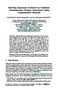
The results in Figure 6 show that, across all training times, networks with N = 100, k = 39 possess chaotic dynamics. Our simulations take networks with various lengths of training time and sample Hamming distances between the actual network state and a perturbed state (in which a certain number of bits from the original state are flipped) at times t and t + 1 for initial perturbation sizes 2, 4, 6, . . . , 20. The Hamming distances between the various perturbed network states and the original state are then calculated after one timestep. This process is completed 1000 times for each network (i.e., each length of training time). Only valid network states (i.e., states where only k neurons are active at a given timestep) are considered. A Derrida plot [7] shows the existence of chaotic dynamics in networks. If the graph of resultant Hamming distance lies above the 45◦ line, this indicates the presence of chaos (since Hamming distance between network states is increasing, i.e., the states are moving “further” apart in the state space). Regardless of training time, networks in our simulation exhibited chaotic behavior. Indeed, little distinction can be seen between the graphs representing various training times (different colored curves in Figure 6). These results make intuitive sense: states with an initial Hamming distance n were more dissimilar after one timestep. These results are consistent with the statistical results of our networks on industrystandard random number generator test suites. Longer training times give rise to 31

Normalized Hamming distance at time t+1

0.35

0.3

0.25

0.2

100 500 1000 5000 10000 15000 25000 50000 75000 100000 45 deg line

0.15

0.1

0.05

0 2

4

6

8 10 12 14 Hamming distance at time t

16

18

20

Figure 6: Derrida Plot showing Hamming Distance (at t) vs. normalized Hamming Distance (at t + 1) for networks with N = 100, k = 39, 2-step refractory period, trained with anti-STDP & IP. The different colored lines represent various training times (values in legend). Lines above the blue 45◦ line show networks whose dynamics operate in a chaotic regime.

32

network dynamics better suited for random number generation. The presence of chaos, though apparently not directly related to training time, does provide a basis for creating dynamics potentially well-suited for random number generation.

9 9.1

Discussion Results of Simulated Networks

Networks trained with anti-STDP & IP (as well as networks trained, then shuffled and retrained with IP) performed on par with industry standard random number generators. These networks also possessed dynamics that expressed several distinct positive characteristics of good pseudo-random number generators. We summarize these results here. 9.1.1

Statistical Results

The performance of our networks for well-chosen parameter sets on pseudo-random number generator test suites indicates that this method of generation produces data that passes most tests to determine “randomness”. Additionally, our networks performed on par with industry-standard pseudo-random number generators. Networks trained with anti-STDP & IP could be useful in areas of statistical simulation, as well as cryptography. In particular, statistical simulation appears a strong candidate for the use of these generated numbers. Though we speculate that it is, we cannot rigorously determine that the update function used in our simulations is indeed a one-way function [4] [5]. Our networks produced sequences of at least 8 × 107 bits (roughly 106 valid “numbers”) that passed statistical tests. A data set of this size would be sufficient for many simulation applications. One aspect of random number generation which has not been stressed up to this point is the question of efficiency. Other industry-standard methods, such as the Blum-Blum-Shub algorithm and the Mersenne Twister (discussed in 4.4.4/5) are simpler, easier to implement, and much faster than our neural networks at generating pseudo-random numbers. The Blum-Blum-Shub algorithm is also a cryptographically strong generator [3]. Our networks, due in large part to the size of the systems involved and their high non-linearity, do not generate data efficiently. However, as stated, they are speculated to be cryptographically strong, and certainly the problem of inverting a network state (i.e., finding f (t) from f (t + 1)) illustrates the difficulty of predicting future output without a knowledge of the update function and its initial state. 33

9.1.2

Limit Cycles & Refractory Period

Empirically, our networks also showed strong performance. In particular, networks trained with anti-STDP & IP resulted in the longest limit cycles for networks with N = 100, k = 1 . . . 8 (see Figure 5). As stated in 8.3, our experiments did not take full advantage of these networks’ potential. For k = 1 . . . 8, we did observe a constant exponential growth in limit cycle length. We believe this behavior has an analogue in the smaller network sizes tested for varying N, k. For good parameter sets based on those results (k ≈ N/5, N/3), we believe any arbitrary network can be constructed that will have good statistical and empirical performance. Indeed, using the values of N, k mentioned above, a well-performing network could be chosen based on the desired application, with increasing N for applications requiring longer output data streams. N=10

3

5

8

2.5 2 1.5

4 3

6 4 2

2 0

5 k N=20

5 k N=25

10

0

60 cycle length

20 15 10 5 10 k

20

40 20 0 0

10 k N=30

20

100 cycle length

25

0 0

cycle length

10

1 0

cycle length

N=15

6 cycle length

cycle length

N=5 3.5

10

20 k

30

50

0 0

10

20

30

k

Figure 7: Graph of limit cycle lengths for networks trained with anti-STDP & IP, N = 5, 10, . . . , 30, k = 1, 3, 5, . . . , N and without a refractory period. Solid red lines represent un-shuffled networks, while blue dashed lines represent shuffled, re-trained with IP.

34

It is important however to mention an aspect of the network that seems to play an integral role in good statistical performance on pseudo-random number generation tests. The built-in refractory period appears to be necessary to produce statistically valid results in the tests performed on our experimental networks. In results not presented in this paper, networks trained with anti-STDP & IP but without a refractory period (in particular in the testing phase) produced results similar to those of networks trained with STDP & IP (i.e., they passed none or essentially no tests). We believe there are several reasons for this. First, the “self-disorganizing” property of the anti-STDP routine is somewhat misleading, in that it does indeed enforce some causality in the network. This causality, under an anti-STDP routine, could be considered a sort of “reverse causality,” in that connections (and subsequent firing) of neurons that initially do not fire consecutively are encouraged. This is essentially the same as the STDP routine, but in the STDP case, neurons that fire consecutively are then encouraged to do so in the future. The anti-STDP does, however, in general cause more neurons in the network to fire because of the k parameter, which limits the number of neurons active at a given timestep. For k  N , this results in the “reverse causality” that affects more neurons that the STDP routine would. This explains in part why networks with k > N/2 do not generate good pseudo-random data. The two-step refractory period, which excludes a neuron from firing until two timesteps after its last activation, forms the two peaks seen in the limit cycle graphs (Figure 4) in 8.3. Figures 7, 8 show limit cycle plots of the same networks shown in Figure 4, but with refractory periods of length 0 (no refractory period) and 3. It is not known exactly why this phenomenon occurs at k ≈ N/5, N/3 for a twostep refractory period. The refractory period, in concert with k, does contribute to the poor performance of the network for large k. It essentially forces an n-step alternation between states, where n is the length of the refractory period+1. Since k is large enough to grab more neurons than otherwise might be active (based on preactivation sums), the refractory period simply excludes that large group of neurons, some of which are picked up again by the k-winner-take-all function. This oscillation occurs quickly for large k and results in the extremely short limit cycles and poor performance of networks trained with these parameter sets. We conclude therefore that a two-step refractory period, with well-chosen k, N is the most effective neural network configuration for producing statistically valid pseudo-random data based on our experiments.

35

9.2

Comparison with other PRNGs / Applications

Our networks, as demonstrated in 7.1, performed as well as other industry-standard pseudo-random number generators. They also performed on par with the networks with random orthogonal weight matrices described in [4]. We draw certain conclusions about potential applications for our neural network-based pseudo-random number generators based on these measures of performance as compared to other generators . Since the update and bit gathering functions of the highly non-linear systems presented in this paper are essentially the same as those presented in [4], we conclude that these networks could be viable generators for use in cryptographic applications. The update functions of both of these systems are suspected to be one-way functions, which provide a cryptographically strong and secure way of generating data. The parity gadget implemented in our networks allows for the extraction of a hard-core predicate, which provides a way to generate secure data from network state [5]. Limit cycles for the networks in [4] were longer than ours for equivalent N , but since we could not practically determine cycle lengths for the networks we used for pseudo-random number generation, we cannot compare cycle lengths for networks that achieved similar statistical test results. As stated above, we believe neural networks trained with anti-STDP & IP represent an effective method for generating pseudo-random data for use in scientific simulation. The results we obtained from statistical testing were nearly identical to those of industry-standard generators well-established for use in simulation. It is well known that all PRNGs, despite good (or even perfect) performance on statistical test suites, possess some statistical weakness. In this respect, our model presents a novel alternative using non-linear systems which possess potential advantages over other, more conventional pseudo-random number generation methods in certain contexts. Our results support the conclusion that the neural networks described in this paper would be an effective, if not efficient, method of pseudo-random number generation.

10

Future Work

Some issues that arose during our experiments merit further investigation. These include different data gathering and generation methods, as well as more thorough analysis and experimentation on several of the key aspects of our neural networks. It is important to determine the lengths of limit cycles for networks with N = 100 and well-chosen k. Finding the cycle lengths of these networks, which we used for pseudo-random number generation, was practically infeasible due to computational 36

N=5

N=10

N=15

7

15

5 4 3 0

10 8 6 4 0

5

cycle length

6

cycle length

cycle length

12

k N=20

5 k N=25

10

10 5 0

10 k N=30

20

300

20 10 0 0

10 k

20

100

cycle length

cycle length

cycle length

30

50

0 0

10

20 k

30

200 100 0 0

10

20

30

k

Figure 8: Graph of limit cycle lengths for networks trained with anti-STDP & IP, N = 5, 10, . . . , 30, k = 1, 3, 5, . . . , N and using a 3-step refractory period. Solid red lines represent un-shuffled networks, while blue dashed lines represent shuffled, re-trained with IP.

37

limitations. A faster computer (or cluster of computers) could be used to make more rigorous estimates about the lengths of limit cycles for these networks. We predict that these results would support our conclusions and show a steady exponential growth in cycle length for increasing N . This determination would then further support our conclusion that limit cycle length is directly related to level of statistical performance on pseudo-random number generator tests. Furthermore, longer simulations of neural networks trained with anti-STDP & IP would allow for a more thorough analysis of data generated later in the simulation run, as well as of the entire data run. This analysis could potentially determine whether our networks do indeed have independently and identically distributed output data across the entire simulation output sequence. Additionally, an analysis of data generated from networks that continue to use plasticity in a post-training phase would be an interesting supplement to our research. Aside from this, more investigation should be done into determining the exact effects of an arbitrary n-step refractory period on the dynamics of our networks.

References [1] Abbott and Nelson. Synaptic plasticity: taming the beast. Nature, 2000. [2] Abdi. A neural network primer. Journal of Biological Systems, 1994. [3] Blum, Blum, and Shub. A simple unpredictable pseudo random number generator. SIAM Journal on Computing, 15(2):364–383, 1986. [4] Yishai M. Elyada and David Horn. Can dynamic neural filters produce pseudorandom sequences? Artificial Neural Networks: Biological Inspirations - ICANN 2005, 2005. [5] Oded Goldreich and Leonid A. Levin. A hard-core predicate for all one-way functions. Proceedings of the twenty-first annual ACM symposium on theory of computing, 1989. [6] Pascal Junod. Cryptographic secure pseudo-random bits generation: The blumblum-shub generator. Unpublished, 1999. [7] Stuart Kauffman. Understanding genetic regulatory networks. International Journal of Astrobiology, 2003.

38

[8] Andreea Lazar, Gordon Pipa, and Jochen Triesch. Time series prediction, fading memory and error correction in recurrent networks shaped by plasticity. Unpublished, 2006. [9] Pierre L’Ecuyer. Random number generation. In Handbook of Computational Statistics, 2004. [10] Pierre L’Ecuyer. Personal correspondence, 2006. [11] Irwin B. Levitan and Leonard K. Kaczmarek. The Neuron: Cell and Molecular Biology. Oxford University Press, 1991. [12] George Marsaglia. Documentation of the diehard test suite. [13] George Marsaglia. diehard website: http://www.stat.fsu.edu/pub/diehard/. [14] Matsumoto. Mersenne twister website: u.ac.jp/∼m-mat/mt/emt.html.

http://www.math.sci.hiroshima-

[15] Matsumoto and Nishimura. Mersenne twister: a 623-dimensionally equidistributed uniform pseudo-random number generator. ACM Transactions on Modeling and Computer Simulation, 8(1):3–30, 1998. [16] NIST. Website of the national institute of standards and technology prng test suite: http://csrc.nist.gov/rng. [17] pLab. Website of plab: http://random.mat.sbg.ac.at/generators/. [18] Rukhin, Soto, Nechvatal, Smid, Barker, Leigh, Levenson, Vangel, Banks, Heckert, Dray, and Vo. A statistical test suite for random and pseudorandom number generators for cryptographic applications. NIST Special Publication 800-22, 2001. [19] Steven H. Strogatz. Nonlinear Dynamics and Chaos. Westview Press, 1994. [20] C. van Vreeswijk and H. Sompolinsky. Chaos in neuronal networks with balanced excitatory and inhibitory activity. Science, 1996. [21] Stefan Wegenkittl. On empirical testing of pseudorandom number generators. Proceedings of the international workshop on Parallel Numerics ’95, 1995. [22] William W. Wu. Generalized shift register pulse sequence generator patent application. Technical report, Communications Satellite Corporation, 1971.

39