12th International Society for Music Information Retrieval Conference (ISMIR 2011)
PULSE DETECTION IN SYNCOPATED RHYTHMS USING NEURAL OSCILLATORS Marc J. Velasco Edward W. Large Center for Complex Systems and Brain Sciences Florida Atlantic University
[email protected],
[email protected]
often correspond to silences. These two attributes define syncopation [3, 12]. Thus, in syncopated rhythms note events are spaced irregularly in time, yet the perceived pulse is regularly timed, and the meter, regularly structured [3, 14]. A goal of theories of pulse perception is to explain how pulse and meter are perceived for musical rhythms in general, and for syncopated rhythms in particular.
ABSTRACT Pulse and meter are remarkable in part because these perceived periodicities can arise from rhythmic stimuli that are not periodic. This phenomenon is most striking in syncopated rhythms, found in many genres of music, including music of non-Western cultures. In general, syncopated rhythms may have energy at frequencies that do not correspond to perceived pulse or meter, and perceived metrical frequencies that are weak or absent in the objective rhythmic stimulus. In this paper, we consider syncopated rhythms that contain little or no energy at the pulse frequency. We used 16 rhythms (3 simple, 13 syncopated) to test a model of pulse/meter perception based on nonlinear resonance, comparing the nonlinear resonance model with a linear analysis. Both models displayed the ability to differentiate between duple and triple meters, however, only the nonlinear model exhibited resonance at the pulse frequency for the most challenging syncopated rhythms. This result suggests that nonlinear resonance may provide a viable approach to pulse detection in syncopated rhythms.
a) pulse
Simple Rhythm ! ! " # # # " # "$ # " # # # " # # # $ $ ! $ $
weak strong
1
b) pulse
2
3
4
1
2
3
4
3-2 Rumba Clave !! " # # " # # # " # # " # " # # # $ $ $ ! $ $
weak strong
1
2
3
4
1
2
3
4
Figure 1. Example rhythms and metrical grid. Our approach is based on the idea that the pulse percieved in a musical rhythm is a neural resonance that arises in sensory [6, 8, 17] and motor cortices [2, 4]. The experience of meter is posited to arise from interaction of neural resonances at differenct frequencies. In this paper we put forth a neurodynamic model of pulse and meter and ask whether it can explain the perception of pulse and meter in highly syncopated rhythms.
1. INTRODUCTION Pulse is a periodicity perceived in a musical rhythm, operationally defined as the frequency at which one would most likely tap along to a rhythm [11]. People also perceive meter, a structural pattern of accents among beats of the pulse [10]. Pulse and meter can be diagrammed using the notation of Lerdahl and Jackendoff [10], in which the metrical grid is composed of beats at multiple related frequencies, with strong beats occurring when beats at multiple frequencies overlap in time. Thus meter organizes beats of the pulse into strong beats and weak beats. In simple rhythms (Figure 1a), note-events occur on strong beats. Rhythms such as the 3-2 Rumba Clave (Figure 1b), although they share the same nominal metrical structure, are more complex. In such rhythms, note-events occur on metrically weak beats, and strong metrical beats
1.1 Neural Oscillation Neural oscillation can arise from the interaction between excitatory and inhibitory neural populations. The canonical model used here was derived, using normal form theory, from the Wilson-Cowan model of the interaction between excitatory and inhibitory neural populations [7, 18]. This model is generic, however, so the responses of the model to musical rhythm are likely to be observed in many other nonlinear oscillator models of rhythm perception.
185
Poster Session 2
1.2 Model
used to model critical oscillations of outer hair cells in the cochlea [5]. When α > 0 (and β < 0), the system exhibits a limit cycle in absence of input; thus, it can oscillate spontaneously. Our canonical model [7] (Eq 3) is an expansion of the Hopf normal form (Eq 2), which includes higher order terms.
Our conceptual model is a network of neural oscillators, spanning a range of natural frequencies, stimulated with an auditory rhythm. The basic concept is similar to signal processing by a bank of linear filters [15], but with the important difference that the processing units are nonlinear, rather than linear resonators. We can describe the behavior of a linear filter using a differential equation (Eq 1), where the overdot denotes differentiation with respect to time. z is a complex-valued state variable; ω is radian frequency. α < 0 is a linear damping parameter. x(t) denotes linear forcing by a timevarying external signal.
z˙ = z(α + iω) + x(t)
(3)
There are again surface similarities with the previous models. The parameters, ω, α and β1 correspond to the parameters of the truncated model. β2 is an additional amplitude compression parameter, and c represents strength of coupling to the external stimulus. δ 1 and δ 2 are frequency detuning parameters. The parameter ε controls the amount of nonlinearity in the system. Most importantly, coupling to a stimulus is nonlinear and has a passive part, P(ε, x(t)) and an active part, A(ε, z), as defined in [7], which produce different higher order resonances, as described in the next section.
(1)
Because z is a complex variable, it has both amplitude and phase. Resonance in a linear system means that the system oscillates at the frequency of stimulation, with amplitude and phase determined by system parameters. As stimulus frequency, ω 0, approaches the oscillator frequency, ω , oscillator amplitude, r = |z|, increases, providing band-pass filtering behavior. In the linear case, oscillator amplitude depends linearly on stimulus amplitude. A common model of nonlinear oscillation is based on the normal form for the Hopf bifurcation (Eq 2).
z˙ = z(α + iω + β|z|2 ) + x(t) + h.o.t.
1.3 Properties of Nonlinear Resonance Equation 3 displays all the behavioral regimes described above – linear, critical and limit cycle – depending on the parameter values chosen. Additionally, Equation 3 can also exhibit a double-limit cycle bifurcation, when α < 0, β1> 0, β < 0 (and ε > 0). Stable states emerge at rest and at a stable limit cycle; an unstable limit cycle separates the two, functioning as a kind of threshold. If the stimulus is strong enough, the threshold will be crossed, the system reaches the stable limit cycle, and oscillation can be maintained even after the stimulus has ceased. Thus an oscillator operating in a double-limit cycle regime can maintain a memory of an oscillating stimulus. Higher-order resonance means that a nonlinear oscillator with frequency f responds to harmonics (2f, 3f, ...), subharmonics (f/2, f/3, ...) and integer ratios (2f/3, 3f/4, ...) of f. If a stimulus contains multiple frequencies, a nonlinear oscillator will respond at combination frequencies (f2 - f1, 2f1 - f2, ...) as well. Higher order resonances follow orderly relationships and can be predicted given stimulus amplitudes, frequencies and phases. This has important implications for understanding the behavior of such systems. The nonlinear oscillator network does not merely transduce signals; it adds frequency information, which can be used to model pattern recognition and pattern completion, among other things. Neural pattern completion based on nonlinear resonance may explain the perception of pulse and meter in syncopated rhythmic patterns [9, 13].
(2)
Note the surface similarities between this form and the linear resonator of Equation 1. Equation 2 can be seen as a generalization of Equation 1, and the two behave the same when β= 0. Again ω is radian frequency, and α is still a linear damping parameter. β < 0 is a nonlinear damping parameter, which maintains stability when α > 0. x(t) denotes linear forcing by an external signal. The term h.o.t. denotes higher-order terms of the nonlinear expansion that are truncated (i.e., ignored) in normal form models. When α = 0 and β < 0, the system is said to be in the critical parameter regime, poised between damped and spontaneous oscillation. The amplitude of the response depends nonlinearly on the input amplitude. Like linear resonators, nonlinear oscillators have a filtering behavior, responding maximally to stimuli near their own frequency. Differences in behavior include extreme sensitivity to weak signals and high frequency selectivity. Critical oscillators have been
2
Permission to make digital or hard copies of all or part of this work for personal or classroom use is granted without fee provided that copies are not made or distributed for profit or commercial advantage and that copies bear this notice and the full citation on the first page. © 2011 International Society for Music Information Retrieval
186
12th International Society for Music Information Retrieval Conference (ISMIR 2011)
Our hypothesis is that in rhythms with no energy at the pulse frequency, pulse arises due to nonlinear resonance in the brain. Significant contributions may also come from instrinsic dynamics and learned connectivity. As a first test of this hypothesis, we ask whether such resonances arise in a canonical nonlinear model.
+,-./0-1-2,
!
!"#
$
$"#
%
%"#
&
&"#
'
'"#
#
#"#
(
("#
)
)"#
*
%
%"#
&
&"#
'
'"#
#
#"#
(
("#
)
)"#
*
%
%"#
&
&"#
'
'"#
#
#"#
(
("#
)
)"#
*
%
%"#
&
&"#
'
'"#
#
#"#
(
("#
)
)"#
*
D0A;
+.!?8@43>0A;
!
" !
!"#$"
!
!%#""
!
!&#""
!
!'#""
!
!(#""
B3**3/C!D04*;!% "#(
"#(
"#'
"#'
"
" !
!"#$"
!
!%#""
!
!&#""
!
!'#""
!
!(#""
E.;F0;/,G!HIJK
Figure 3. Experiment 1 results. A subset of the rhythms presented with both an FFT of the stimulus (black) and the amplitudes of responding nonlinear oscillators (gray). The two networks were connected as shown in Figure 4. Tonotopic connections between the networks allow Network 1 to drive Network 2. Next, in each network, internal connectivity coupled patches of oscillators to other patches exhibiting small integer ratio frequency relationships, 1:3, 1:2, 1:1, 2:1, 3:1. These connections are assumed to be learned by exposure to Western rhythms, in which duple and triple meters are common. Connectivity from Network 2 to Network 1 was inhibitory.
3. EXPERIMENT 2 3.1 Stimuli & Method
3.3 Results
The stimuli methods used in Experiment 2 were the same as in Experiment 1.
Across the rhythms presented, Network 1 behaved similarly to the previous experiment, responding to frequencies present in the simulus rhythms, and also adding nonlinear resonances. Example of Network 2 responses are shown in Figure 5. Due to its thresholding properties, Network 2 responded to a subset of frequencies present in the Network 1. Importantly, Network 2 almost always responded at the pulse frequency. Moreover, the amplitude at 2 Hz was unexpectedly strong given the relatively weak responses observed in Experiment 1.
3.2 Model The model was based on the same oscillator equations as used in Experiment 1. The key difference was that in Experiment 2, the model consisted of two networks interacting with each other. Network 1 had the same parameters as used in Experiment 1. The oscillators in Network 2 were tuned to exhibit double limit cycle bifurcation behavior (α = 0.3, β1 = 1, β2 = -1, and ε = 1), and thus exhibited both threshold and memory properties.
188
12th International Society for Music Information Retrieval Conference (ISMIR 2011)
Stimuli Rhythm Isochronous 4/4 3/4 Son Clave Rumba Clave Hard Clave Missing Pulse 1 Missing Pulse 2 Missing Pulse 3 Missing Pulse 4 Missing Pulse 5 Missing Pulse 6 Missing Pulse 7 Missing Pulse 8 Missing Pulse 9 Missing Pulse 10
729:*+.9+,2. !"#$%&'
5)+.2)'6
!"#$%&(
/.+01234%
/.+01234$ E88.2.)+
788.2.)+ /.+01234$
;1)).9+*'++.2)? 788.2.)+
@21G4/
[email protected],.)9*.? 4
4!"# 4$"! 4%"!
&'()*+,-.
F14/
[email protected],.)9*.?
4!"%#
4B"! 4C"! $D"!
!"% !"$# !"$ !"!# ! 4!"%#
4
4!"#
4$"!
4%"!
4B"!
4C"!
$D"!
@2.A,.)9= !
5)+.2)'6
!"!#
4$"!
4%"!
!"$
4B"!
4C"!
$D"!
4!"# 4$"! 4%"!
&'()*+,-.
F14/
[email protected],.)9*.?
4!"%# 4!"# 4!"%#
4B"! 4C"! $D"!
!"% !"$# !"$ !"!# ! 4!"%#
4
4!"#
4$"!
4%"!
4B"!
4C"!
$D"!
Network 2 Active Frequencies (Hz) 1/2 2/3 1 2 4 Other x x x x x x x x x x x x 0.62 x x x 0.62, 0.88 x x 0.62, 1.24 x x x 0.62 x x 0.63, 0.75 x x 0.62 x x 0.62, 0.88, 1.12 x x x x 0.62, 0.75, 1.24 x x 0.62, 0.75 x x 0.62, 0.75 x x x 0.75 x x 0.75 x x 0.63, 0.75, 1.26
@2.A,.)9= !"!% !"!B !"!D !"!C !"$
Table 1. Summary of results for Experiment 2. Shaded cells identify frequencies which would be expected to have a resonance for the rhythm based on meter. Populated cells (x) show which resonant frequencies were active in Network 2.
&'()*+,-.
Figure 4. Network architecture for models used in both experiments. )*+,-.+/+0*
most of the rhythms (the one exception was the canonical 3/4 rhythm, whose slower metrical frequency was 0.67 Hz). The results of the two-network model can be seen in Table 1. Highlighted cells show the frequencies at which response peaks would be expected based on the meter. Populated cells show whether or not response peaks were observed at given frequencies. For all but one rhythm, a response was seen at the pulse frequency of 2 Hz. For the canonical rhythms, response peaks were always found at the expected frequencies and at no others. This set of hierarchically related frequencies may correspond to a perception of meter. For the missing pulse rhythms, response peaks were found most consistently at the pulse frequency and its first harmonic at 4 Hz. At lower frequencies, the results differed from standard metrical predictions. This may explain why people sometimes have difficulty entraining periodic taps with highly syncopated stimuli. In previous experiments, level of syncopation was found to be a good predictor of pulse-finding difficulty; syncopation causes off-beat taps and some switches between on-beat and off-beat tapping [14, 16].
% "#$ "
!"#$"
3:*D+/*:!E4D8