Quantum Control Algorithm of Robust KB Self-Organization Process Based on Quantum Fuzzy Inference S.V. Ulyanov MCG “Quantum,” Moscow,
[email protected] Abstract Different models of self-organization processes are described from physical, information, and algorithmic (quantum computing) point of view. Role of quantum correlation types and information transport in self-organization of structure type design is discussed. A generalized quantum algorithm (QA) design of self-organization processes is developed. Particular case of this approach (based on early developed quantum swarm model) is discussed. The physical interpretation of self-organization control process on quantum level is introduced based on the information model of the exchange and extraction of quantum (hidden) value information from/between classical particle’s trajectories in particle swarm. New types of quantum correlations (as behavior control coordinator) and information transport (value information) between particle swarm trajectories are introduced. Quantum Fuzzy Inference (QFI) model is introduced based on thermodynamics and information-theoretic measures of agent interactions in communication space between macro- and micro-levels (the entanglement-based correlations in an active system represented by a collection of intelligent agents). From computer science viewpoint, QA of QFI model plays the role of the information-algorithmic and SWplatform support for design of self-organization process. Physically, QFI supports optimal thermodynamic trade-off between stability, controllability and robustness in self-organization process. The dominant role of self-organization in robust knowledge base (KB) design of intelligent fuzzy controllers (FC) for unpredicted control situations is discussed. Key words: Self-organization, correlation, quantum information, quantum control algorithm, quantum fuzzy inference (QFI), thermodynamic trade-off, robust KB, intelligent control
Introduction In recent years, the concept of self-organization has been used to understand collective behavior of human being society, animals, ant’s, bird’s, bacteria’s colonies, quantum dots etc. The central tenet of self-organization is that simple repeated interactions between individuals can produce complex adaptive patterns at the level of the group. Inspiration comes from patterns seen in physical systems, such as spiraling chemical waves, which arise without complexity at the level of the individual units of which the system is composed. The suggestion is that biological structures such as termite mounds, ant trail networks and even human crowds can be explained in terms of repeated interactions between the animals and their environment, without invoking individual complexity. As examples, a flock of birds twisting in the evening light; a fish school wincing at the thought of a predator; the cram to leave an underground station; ants marching in an endless line; the stop and start traffic jams; the quiet hum of a honey bee hive; the pulsating roar of a football crowd; a swarm of locusts flying across the desert; or even the bureaucracy of the European Union, USA, Japan, China, and Russia. In all these examples, the individual is submerged as the group takes on a life of its own. The individual units do not have a complete picture of their position in the overall structure and the structure they create has a form that extends well beyond that of the individual units. Q: Beyond the fact that individuals produce collective patterns, is there anything more specific we can say about these phenomena we have labeled self-organized? The answer to this question lies in the relationship between similarities in the rules governing and the patterns generated by very different systems. A general characteristic of self-organizing systems is as following: they are robust or resilient. This means that they are relatively insensitive to perturbations or errors, and have a strong capacity to restore themselves, unlike most human designed systems. One reason for this fault-tolerance is the redundant, distributed organization: the non-damaged regions can usually
make up for the damaged ones. Another reason for this intrinsic robustness is that selforganization thrives on randomness, fluctuations or “noise”. A certain amount of random perturbations will facilitate rather than hinder self-organization. A third reason for resilience is the stabilizing effect of feedback loops. The present report reviews and analyzed its most important engineering concepts and principles of self-organization that can be used in design of robust intelligent control systems [1]. We choice for analysis of common futures as Benchmarks the following examples [2 - 19]: (1) Pedestrian behavior and self-organization; (2) ‘‘Phantom panics’’ and self-organization; (3) Self-organization of traffic flow models; (4) Swarm self-organization and swarm intelligence (SI): 4.1. Applications of SI and ant colony self-organization; 4.2. Agent-Based Models (ABM); 4.3. Quantum cooperation of two insects; 4.4. Engineered self-organization of a bacteria colony; (5) Self-organization in nano-scale structures: Quantum corrals. In Appendix, briefly physical principles of these self-organization models are described. In these examples self-organizational processes begin with the amplification (through positive feedback) of initial random fluctuations. This breaks the symmetry of the initial state, but often in unpredictable (but operationally equivalent) ways. That is, the job gets done, but hostile forces will have difficulty predicting precisely how it gets done. For example, a key issue in nanotechnology is the development of conceptually simple construction techniques for the mass fabrication of nano-scale structures reaching down to the atomic scale. At this level the conventional top-down fabrication paradigm becomes excessively energy-intensive, wasteful, expensive and complicated. The natural alternative is self-organized growth, where nano-scale arrangements are built from their atomic and molecular constituents by processes intrinsically providing structural organization. This approach is based on a detailed understanding of the microscopic pathways of diffusion, nucleation and aggregation. The hierarchy in the migration barriers as well as the non-uniform strain fields induced by mismatched lattice parameters can be translated into geometric order and well defined shapes and length scales of the resulting aggregates. In self-organizing systems the relation between cause and effect is much less straightforward: small causes can have large effects, and large causes can have small effects. This non-linearity can be understood from the relation of feedback that holds between the system’s components. Each component (e.g. a spin) affects the other components, but these components in turn affect the first component. Thus the cause-and-effect relation is circular: any change in the first component is feedback via its effects on the other components to the first component itself. Remark. The above mentioned feedback is one of important component in advanced control theory and can have two basic values: positive or negative. Feedback is said to be positive if the recurrent influence reinforces or amplifies the initial change. In other words, if a change takes place in a particular direction, the reaction being feedback takes place in that same direction. Feedback is negative if the reaction is opposite to the initial action, that is, if change is suppressed or counteracted, rather than reinforced. Negative feedback stabilizes the system, by bringing deviations back to their original state. Positive feedback, on the other hand, makes deviations grow in a runaway, explosive manner. It leads to accelerated development, resulting in a radically different configuration. Thus, physically, a process of self-organization typically starts with a positive feedback phase, where an initial fluctuation is amplified, spreading ever more quickly, until it affects the complete system. Once all components have “aligned” themselves with the configuration created by the initial fluctuation, the configuration stops growing: it has “exhausted” the available resources. Now the system has reached equilibrium (or at least a stationary state). Since further growth is no longer possible, the only possible changes are those that reduce the dominant
configuration. However, as soon as some components deviate from this configuration, the same forces that reinforced that configuration will suppress the deviation, bringing the system back to its stable configuration. This is the phase of negative feedback. In more complex self-organizing systems, there will be several interlocking positive and negative feedback loops, so that changes in some directions are amplified while changes in other directions are suppressed. This can lead to very complicated, difficult to predict behavior. These self-organized systems have different physical nature but can be described in general form based on developed quantum control algorithm of self-organization [11]. Analysis of self-organization models gives us the following results. Models of self-organization are included natural quantum effects and based on the following information-thermodynamic concepts: (i) macro- and micro-level interactions with information exchange (in ABM micro-level is the communication space where the inter-agent messages are exchange and is explained by increased entropy on a micro-level); (ii) communication and information transport on micro-level (“quantum mirage” in quantum corrals); (iii) different types of quantum spin correlation that design different structure in self-organization (quantum dot); (iv) coordination control (swam-bot and snake-bot). Natural evolution processes are based on the following steps [2 - 7]: (i) templating; (iii) selfassembling; and (iii) self-organization. According quantum computing theory in general form every QA includes the following unitary quantum operators: (i) superposition; (ii) entanglement (quantum oracle); (iii) interference. Measurement is the fourth classical operator. [It is irreversible operator and is used for measurement of computation results]. Quantum control algorithm of self-organization that developed below [11] is based on QFI models. QFI includes these concepts of self-organization and has realized by corresponding quantum operators. Structure of QFI that realize the self-organization process is developed. QFI is one of possible realization of quantum control algorithm of self-organization that includes all of these features: (i) superposition; (ii) selection of quantum correlation types; (iii) information transport and quantum oracle; and (iv) interference. With superposition is realized templating operation, and based on macro- and micro-level interactions with information exchange of active agents. Selection of quantum correlation type organize self-assembling using power source of communication and information transport on micro-level. In this case the type of correlation defines the level of robustness in designed KB of FC. Quantum oracle calculates intelligent quantum state that includes the most important (value) information transport for coordination control. Interference is used for extraction the results of coordination control and design in online robust KB. The developed QA of self-organization is applied to design of robust KB of FC in unpredicted control situations. Main operations of developed QA and concrete examples of QFI applications are described.
1. Principles and Physical Model Examples of Self-Organization The theory of self-organization, learning and adaptation has grown out of a variety of disciplines, including quantum mechanics, thermodynamics, cybernetics, control theory and computer modeling. The present section reviews its most important definitions, principles, model descriptions and engineering concepts that can be used in design of robust intelligent control systems. 1.1. Definitions and main properties of self-organization Self-organization is defined in general form as following [2, 3, 5, 6]: The spontaneous emergence of large-scale spatial, temporal, or spatiotemporal order in a system of locally interacting, relatively simple components Self-organization is a bottom-up process where complex organization emerges at multiple levels from the interaction of lower-level entities. The final product is the result of nonlinear
interactions rather than planning and design, and is not known a priori. Contrast this with the standard, top-down engineering design paradigm where planning precedes implementation, and the desired final system is known by design. Self-organization can be defined as the spontaneous creation of a globally coherent pattern out of local interactions. Because of its distributed character, this organization tends to be robust, resisting perturbations. The dynamics of a self-organizing system is typically nonlinear, because of circular or feedback relations between the components. Positive feedback leads to an explosive growth, which ends when all components have been absorbed into the new configuration, leaving the system in a stable, negative feedback state. Nonlinear systems have in general several stable states, and this number tends to increase (bifurcate) as an increasing input of energy pushes the system farther from its thermodynamic equilibrium. To adapt to a changing environment, the system needs a variety of stable states that is large enough to react to all perturbations but not so large as to make its evolution uncontrollably chaotic. The most adequate states are selected according to their fitness, either directly by the environment, or by subsystems that have adapted to the environment at an earlier stage. Formally, the basic mechanism underlying self-organization is the (often noise-driven) variation which explores different regions in the system’s state space until it enters an attractor. This precludes further variation outside the attractor, and thus restricts the freedom of the system’s components to behave independently. This is equivalent to the increase of coherence, or decrease of statistical entropy, that defines self-organization. The most obvious change that has taken place in systems is the emergence of global organization. Initially the elements of the system (spins or molecules) were only interacting locally. This locality of interactions follows from the basic continuity of all physical processes: for any influence to pass from one region to another it must first pass through all intermediate regions. In the self-organized state, on the other hand, all segments of the system are strongly correlated. This is most clear in the example of the magnet: in the magnetized state, all spins, however far apart, point in the same direction. Correlation is a useful measure to study the transition from the disordered to the ordered state. Locality implies that neighboring configurations are strongly correlated, but that this correlation diminishes as the distance between configurations increases. The correlation length can be defined as the maximum distance over which there is a significant correlation. When we consider a highly organized system, we usually imagine some external or internal agent (controller) that is responsible for guiding, directing or controlling that organization. The controller is a physically distinct subsystem that exerts its influence over the rest of the system. In this case, we may say that control is centralized. In self-organizing systems, on the other hand, “control” of the organization is typically distributed over the whole of the system. All parts contribute evenly to the resulting arrangement. Remark. Although centralized control does have some advantages over distributed control (e.g. it allows more autonomy and stronger specialization for the controller), at some level it must itself be based on distributed control. For example, the behavior of human being body can be best explained by studying what happens in his brain, since the brain, through the nervous system, controls the movement of muscles. However, to explain the functioning of brain, we can no longer rely on some “mind within the mind” that tells the different brain neurons what to do. This is the traditional philosophical problem of the homunculus, the hypothetical “little man” that had to be postulated as the one that makes all the decisions within mental system. Any explanation for organization that relies on some separate control, plan or blueprint must also explain where that control comes from otherwise it is not really an explanation. The only way to avoid falling into the trap of an infinite regress (the mind within the mind within the mind within...) is to uncover a mechanism of self-organization at some level. The brain illustrates this principle nicely. Its organization is distributed over a network of interacting neurons. Although different brain regions are specialized for different tasks, no neuron or group of neurons has overall control.
This is shown by the fact that minor brain lesions because of accidents, surgery or tumors normally do not disturb overall functioning, whatever the region that is destroyed. As mentioned in Introduction a general characteristic of self-organizing systems is as following: they are robust or resilient. This means that they are relatively insensitive to perturbations or errors, and have a strong capacity to restore themselves, unlike most human designed systems. One reason for this fault-tolerance is the redundant, distributed organization: the non-damaged regions can usually make up for the damaged ones. Another reason for this intrinsic robustness is that self-organization thrives on randomness, fluctuations or “noise”. A certain amount of random perturbations will facilitate rather than hinder self-organization. A third reason for resilience is the stabilizing effect of feedback loops. Many self-organizational processes begin with the amplification (through positive feedback) of initial random fluctuations. This breaks the symmetry of the initial state, but often in unpredictable but operationally equivalent ways. That is, the job gets done, but hostile forces will have difficulty predicting precisely how it gets done. Stigmergy is an important principle of self-organization, seen for example in wasp nest building and spider web construction. It refers to a way of coordinating a collective construction process so that the project itself contains the information necessary to guide the actions of the workers. Scientific research has shown the pervasiveness of self-organization in the natural world, from nonliving systems, through microorganisms, to species of all degrees of complexity, including human beings. This research has demonstrated how comparatively simple interactions, often among organisms with limited cognitive capacities, can solve complex command, control, and coordination problems in order to promote their survival and to accomplish their ends. The behavior of these species is more robust, flexible, and adaptive than they would be if they were not based on self-organization. Self-organization is especially attractive as an approach to the robust, flexible, and adaptive implementation of command, control, and communication systems of enormous potential value to military operations, homeland security, and public safety. With this increased knowledge of natural self-organization, has come improved understanding of various general principles that can be applied to artificial intelligent systems to achieve the same benefits. In past research, a variety of simulation studies have shown that these principles of self-organization can be applied in artificial systems, which may be quite different from the natural systems in which the principles were originally observed. 1.2. Principles and Models of Self-Organization Self-organization has long been a matter of immense interest and research in sociology, anthropology, physics and many other fields. Though the principles of self-organization can be inducted from almost all walks of human, plant and animal lives [2 - 7], and in computer science [8] can be used. It is most evident in ant and termites colonies [9] or self-engineering capabilities of bacteria [10]. Self-organization has been used to explain the formation of cities, software, brain cells and many natural phenomena in human societies. Though the principle is used to explain other phenomena, the concept itself is continuously evolving. Self-organization phenomena are correlated with information transport and thermodynamics processes [5 - 7, 15 - 17]. The term self-organizing systems refers to a class of systems that are able to change their internal structure and their function in response to external circumstances. By self-organization it is understood that elements of a system are able to manipulate or organize other elements of the same system in a way that stabilizes either structure or function of the whole against external fluctuations. Traditionally three forms of self-organization are analyzed as following: (1) stigmergy; (ii) reinforcement mechanisms; and (iii) cooperation. The amplification phenomena founded in stigmergic process or in reinforcement process are different forms of positive feedbacks that play a major role in building group activity or social organization. Cooperation is a functional form for self-organization because of its ability to guide local behaviors in order to obtain a relevant collective one.
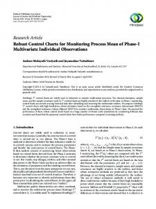
Self-organization mechanisms guide the behavior of the local entities of a collective. Consequently these approaches allow a drastic reduction of the solution search space compared to global search algorithms. Working on self-organization implies the creation of disorders inside a collective in order to obtain later a more relevant response of the system faced with unexpected events. From an engineering point of view it could be interesting to propose global systems gauges able to link disorder and relevance behavior at the system macro-level. Self-organization essentially refers to a spontaneous, dynamically produced (re-)organization. Several definitions corresponding to the different self-organization behaviors: (1) Swarm intelligence (SI); (2) Decrease of entropy; (3) Autopoiesis; (4) Artificial systems; (5) Emergence. Remark. Many natural systems show self-organization property (e.g. galaxies, planets, chemical compounds, cells, organisms and societies). Traditional scientific fields attempt to explain these features by referencing the micro properties or laws applicable to their component parts, for example gravitation or chemical bonds. Furthermore, self-organization implies organization, which in turn implies some ordered structure and component behavior. In this respect, the process of self-organization changes the respective structure and behavior, and a new distinct organization is self-produced. Emergence is the fact that a structure, not explicitly represented at a lower level, appears at a higher level. In the case of dynamic self-organizing systems, with decentralized control and local interactions, intimately linked with selforganization is the notion of emergent properties. The ants actually establish the shortest path between the nest and the source of food. However in the general case, self-organization can be witnessed without emergence and vice-versa. 1.2.1. Principles of self-organization. Over the last half a century, much research in different areas has employed self-organizing systems to solve complex control problems. However, there is as yet no general framework for constructing self-organizing systems. Different vocabularies are used in different areas, and with different goals. (Detail description of self-organization principles and different natural/man-manned models of self-organization structures are presented in [3, 5 - 7, 11]). The essence of self-organization is that system structure often appears without explicit pressure or involvement from outside the system. In other words, the constraints on form (i.e. organization) of interest to us are internal to the system, resulting from the interactions among the components and usually independent of the physical nature of those components. The organization can evolve in either time or space, maintain a stable form or show transient phenomena. General resource flows within self-organized systems are expected (dissipation), although not critical to the concept itself. Remark: Related works. The term self-organization has been used in different areas with different meanings, as is cybernetics, social-economic systems, thermodynamics, biology, mathematics, computing, information theory, synergetic, and others (for a general overview, see [11], and References there). However, the use of the term is subtle, since any dynamical system can be said to be self-organizing or not, depending partly on the observer: If we decide to call a “preferred” state or set of states (i.e. attractor) of a system “organized”, then the dynamics will lead to a self-organization of the system. A practical notion will suffice: A system described as self-organizing is one in which elements interact in order to achieve dynamically a global function or behavior [20]. This function or behavior is not imposed by one single or a few elements, nor determined hierarchically. It is achieved autonomously as the elements interact with one another. These interactions produce feedbacks that regulate the system. Many nonliving physical and chemical systems have the capacity to generate order from chaos. This capacity is known as self-organization. Self-organized systems can evolve by small parameter shifts that produce large changes in outcome. A common misconception about self-organization in biological systems is that it represents an alternative to natural selection. Self-organization usually relies on four basic ingredients: (i) Positive feedback; (ii) Negative feedback; (iii) Balance of exploitation and exploration; and (iv) Multiple interactions. All the previously mentioned examples of complex systems fulfill the definition of self-organization. Figure 1 shows these principles of self-organization in ant colony.
Ant swarm self-organization Path Way with Feed-backs and Decision Making
Figure 1: Feedbacks loops and collective choice of one food source (bifurcation) [9] When two food sources of equal quality are offered to an ant society, only one becomes selected through the concurrent influence of positive (in green) and negative (in red) feedback loops. Examples of such feedbacks are given in the Figure 1. Depending on these feedbacks, the trail amount and hence the probability for newly coming ants to choose one path (either P1 or P2) at the bifurcation point will change over time and will ultimately lead to the collective choice of one food source. More precisely, the question can be formulated as follows. Q: When is it useful to describe a system as self-organizing? This will be when the system or environment is very dynamic and/or unpredictable. If we want the system to solve a problem, it is useful to describe a complex system as selforganizing when the “solution” is not known beforehand and/or is changing constantly. Then, the solution is dynamically strived for by the elements of the system. In this way, systems can adapt quickly to unforeseen changes as elements interact locally. In theory, a centralized approach could also solve the problem, but in practice such an approach would require too much time to compute the solution and would not be able to keep the pace with the changes in the system and its environment. In engineering, a self-organizing system would be one in which elements are designed in order to solve dynamically a problem or perform a function at the system level. Thus, the elements need to divide, but also integrate, the problem. For example, a swarm of robots will be conveniently described as self-organizing, since each element of the swarm can change its behavior depending on the current situation. It should be noted that all engineered self-organizing systems are to a certain degree autonomous, since part of their actual behavior will not be determined by a designer. In order to understand self-organizing systems, two or more levels of abstraction should be considered: elements (lower level) organize in a system (higher level), which can in turn organize with other systems to form a larger system (even higher level).
The understanding of the system’s behavior will come from the relations observed between the descriptions at different levels. Note that the levels, and therefore also the terminology, can change according to the interests of the observer. For example, in some circumstances, it might be useful to refer to cells as elements (e.g. bacterial colonies); in others, as systems (e.g. genetic regulation); and in others still, as systems coordinating with other systems (e.g. morphogenesis). A system can cope with an unpredictable environment autonomously using different but closely related approaches: — Adaptation (learning, evolution). The system changes its behavior to cope with the change. — Anticipation (cognition). The system predicts a change to cope with, and adjusts its behavior accordingly. This is a special case of adaptation, where the system does not require experiencing a situation before responding to it. — Robustness. A system is robust if it continues to function in the face of perturbations. This can be achieved with modularity, degeneracy, distributed robustness, or redundancy. Successful self-organizing systems will use combinations of these approaches to maintain their integrity in a changing and unexpected environment. Adaptation will enable the system to modify itself to “fit” better within the environment. Robustness will allow the system to withstand changes without losing its function or purpose, and thus allowing it to adapt. Anticipation will prepare the system for changes before these occur, adapting the system without it being perturbed. 1.2.2. Elements of self-organization. We can see that all of them should be taken into account while engineering self-organizing intelligent systems. 1. Interacting components. The components provide the substrate for organization of higherlevel structures. Interaction/communication is necessary for creating linkages to assemble larger structures. Example components are molecules, cells, agents, etc. Example interactions are excitation, inhibition, sensing, attraction, repulsion, etc. 2. Constructive processes. Needed to build larger structures from the components, e.g., reproduction, aggregation, crystallization, copying, growth, recombination, ramification, etc. 3. Destructive processes. Needed to tear down existing (possibly suboptimal or unwanted) structures to make room for new ones, e.g., death, fragmentation, dissolution, division, mixing, turbulence, noise, etc. 4. Autocatalysis/positive feedback. Needed to reinforce and drive the construction of useful structures, e.g., splits encouraging more splitting to create a complex branching structure. 5. Homeostasis/negative feedback. Needed to prevent runaway structure formation (e.g., structures beyond a certain size becoming non-receptive to further addition or even unstable). 6. Nonlinearity. Needed to magnify some effects and squelch others in order to produce complex structure. Examples include thresholds, unimodal and multimodal dependencies, saturation, and amplification underlying the constructive, destructive and feedback processes. What is Emergence? The appearance of large-scale collective order that cannot be described completely in terms of the individual system components, e.g., meaning from a collection of words, a society from a collection of individuals, a wave from a collection of particles, a picture from a collection of pixels. Emergence seeks to move beyond pure reductionism without resorting to metaphysical explanations, e.g., in explaining phenomena such as intelligence and life. Complex adaptive systems exhibit spontaneous emergence at many levels of description. 1.2.3. Elements of engineering self-organization design and its role in design of robust intelligent control. Let us consider main approach in engineering philosophy of control design. Traditional top-down approach: (1) Consider all possibilities; (2) Develop a very careful design; (3) Thoroughly test the design to verify performance; (4) Implement and test a prototype; (5) Carefully replicate the verified design to ensure reliability. This approach relies on anticipation of all eventualities, meticulous design, thorough testing, and exact replication to obtain the desired level of performance. It works best in well-understood, predictable and relatively simple environments.
Self-organized bottom-up approach: (1) Provide the basic elements/components needed; (2) Let the components interact among themselves and with the environment to organize through an iterative process of creative exploration and selective destruction. This approach produces good designs by multi-scale, parallel, intelligent random search through the space of possibilities. It is appropriate (necessary) for large-scale complex systems operating in complex, dynamic, unpredictable environments, e.g., the real world. Key Difference Top-Down: Every aspect of the system at all levels is carefully designed and evaluated (a) Non-scalable in cost, time, effort, reliability; (b) Critically dependent on component reliability; (c) Inflexible in response to novel conditions. Bottom-Up: Only the basic “simple and cheap” components are designed; the rest of the system organizes itself: (a) Inherently scalable; (b) Flexible, robust, versatile, expandable, evolvable. What do complex adaptive systems buy us? 1. Scalability: The system can grow much larger because no one needs to keep track of everything; 2. Flexibility: The system can change as needed simply by individual agents changing their behavior; 3. Versatility: The system can be used in many different situations without redesign; 4. Expandability: More agents can be added to the system without redesign; 5. Robustness: The system can withstand changes and even loss of individual agents This is a new kind of engineering: (1) We’re no longer designing the system; (2) We’re engineering the possibility for the system to arise; (3) This will work for some applications and not for others. Why do we need to build complex adaptive systems? To obtain systems with attributes such as intelligence, adaptively, robustness, scalability, and flexibility for operation in complex, dynamic and uncertain environments e.g., battlefields, disaster areas, hazardous regions, ocean floors, outer space, etc. To create very large-scale or fine-grained systems where standard design, control, and analysis methods break down for capacity reasons, e.g., sensor networks with millions of nodes, swarms of micro-satellites, etc. To control other complex adaptive systems, e.g., traffic networks, communication networks, biological systems, etc. Self-organization may seem to contradict the second law of thermodynamics that captures the tendency of systems to disorder. The “paradox” has been explained in terms of multiple coupled levels of dynamic activity [the Kugler-Turvey model (Kugler and Turvey, 1987)] selforganization and the loss of entropy occurs at the macro-level, while the system dynamics on the micro-level generates increasing disorder [11, 12, 13, 16, 17]. In [11] are considered five examples of self-organization processes in dynamic systems with different scale dimensions. These examples help to understand main ideas of self-organization and find mutual components of quantum control algorithm of self-organization design. In next sections are considered the structure of this quantum design algorithm and its application to design of robust knowledge base in intelligent FCs. Simulation results are considered on examples of essentially non-linear dynamic system control objects.
2. Quantum Control Algorithm of Self-Organization Processes Let us consider the common parts of models of self-organization processes discussed in Introduction and Section 1. Main steps of generalized (bio-inspired) self-organization processes are as following: - First step is a templating that is organization of component by a template;
- The second step is a self-assembly with control via conformation; and - The third step is a self-organization as collective behavior of interactive (possible selfassembly) components. From the description of qualitative properties of these models we can extract common parts. Main common parts of self-organization processes (described in details in [11]) are as following: (1) Presence of correlation (spatial, temporal, or spatiotemporal types); (2) Random search in design process of a new structure in accordance with initial state and fixed correlation type; (3) Robustness of final new structure; (4) Flexibility of self-organized structure. These common parts are used in bio-inspired and man-made self-organization process (see, Figure 2).
Steps of Bio-Inspired Self-Organization Evolution 1. Templating Organization of molecular component by a template
2. Self-assembly Molecular self-assembly; Control via conformation
3. Self-organization Spatial Quantum correlation
Collective behavior of interactive (possible self-assembly) components
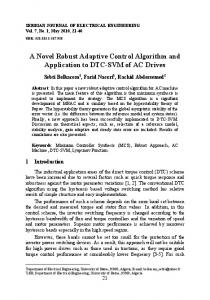
Figure 2: Structure of self-organization processes in things natural and things manmade and self-organization evolution Figure 2 shows also the structure and the main steps (right column) of bio-inspired selforganization processes in things natural and things man-made.
2.1. General Structure of QA of Self-Organization Processes Figure 3 shows the general structure of QA for logical design of bio-inspired selforganization process (see, Figure 2) that includes these common parts.
Algorithmic Level
Natural Decoding of Solution & Answer
Final State
New Self-Organized Robust Structure
Decision Making
Operator Vector (Templating of Operator (Self-assembly) structure) components (self-organization)
Evolution Dynamic Problem-Oriented Correlation Initial State Classical, Quantum, or Mixed Types Random (Classical/Quantum) Search Genetic Inspired Initial Structure Design process
Action of operator
Algorithmic description
Search
Action of operator States with hidden Information
Choice
Coding of Problem
Algorithm design of Self-Organization with Problem-Oriented Operators
Figure 3: Quantum Algorithm of logical design of bio-inspired self-organization process It is a QA design of self-organization with problem-oriented quantum operators: - First step of algorithm, initial states are vector-state that describes component’s templating of future designed structure. From bio-inspired structure point of view it is genetic inspired initial structure of evolution process; from computer science stand viewpoint it is coding of problem searching solution. It is well-known in computer science that vector and matrix can be presented using quantum state: The quantum representation of vector and matrix may be the base of quantum data structure (for compression presentation of massive classical data [21] in templating); - On second step of algorithm a self-assembly process is used (from bio-inspired structure point of view); from computer science stand viewpoint it is a decision-making process on choice of problem-oriented correlation. An action of correlation operator on initial state in templating prepare a structured assemble of components with hidden possible solutions of design structure; - Evolution dynamic realize a self-organization process of new structure design on the third step. Algorithmic description of self-organization process is a random quantum search process of hidden solution in self-assembly structure and acts as corresponding operator on self-assembly structure; - Natural decoding of searching solution is given the answer about final state of a new selforganized structure. The described algorithm is in general a quantum control design algorithm that includes all operation from general structure of QA. Remark. In this section we briefly consider analogy with structure of a QA [22, 23]. In the following section, further concepts of quantum computing will be introduced that will be necessary to apply the described methodology. General structure of QA consists from three quantum as superposition, entanglement (quantum correlation) and interference. Classical measurement gives the final result of quantum computation. Superposition operation is realized
by Hadamard transform, entanglement is realized by CNOT-operation or by quantum oracle, and interference is realized by QFT-operator. Main goal of QA applications is the study and search of qualitative properties of functions as the solution of problem. Initial states are coding of function property. Superposition describes the generalized searching space; a quantum oracle finds the searching solution; with interference operator and classical measurement the searching solution is extracted. The method of collective behavior (swarm method) is the simplest and most evident way for the algorithmization of quantum models. The passage from the single particle to the swarm of its samples seems to be the easiest way to overcome contra intuitiveness featured to quantum theory. With some additional suppositions a swarm method gives the algorithm of simulation of the dynamics with linear complexity of the number of particles. These additional suppositions lay in the framework of the basic idea of algorithmic approach the limitation of the memory and time for the simulation [1, 24]. Figure 4 shows the general structure of QA [11].
Background for Applications of Quantum Computing QCO Answer
SCO
Quantum output Quantum Gate Design
Classical input
Problem
fin Interference Quantum Oracle Superposition initial Quantum Massive Parallel Computations
Function property
Quantum Fourier Transform (QFT)
Qualitative Properties of Functions
Problem-Oriented Operator
Hadamard Transform
Property coding
Quantum Oracle is Black Box
Figure 4: General structure of quantum algorithm The superposition is that we should treat as realizable only states of the system S S1 S2 , S1 sup S2 of the form [24]
S j Sj1 Sj2 ,
(2.1)
j
where S11 , S21 , and S12 , S22 are orthonormal basis in space of states of subsystems S1 and S2 correspondingly, and each of these basic states has the same form, with some depth of nesting. Factually, this is one particle states, where the entanglement is distributed among the particles sequentially nested in each other. The quantum swarm model of self-organization was described in [1]. Remark. Based upon quantum entanglement, several paradigms of self-organization (such as inverse diffusion, transmissions of conditional information, decentralized coordination, cooperative computing, competitive games, and topological evolution in active systems) can be
introduced and discussed. This result was motivated by recent discovery and experimental verification of the most fundamental and still mysterious phenomenon in quantum mechanics: quantum entanglement. Formally, quantum entanglement as well as associated with it quantum non-locality follows from the Schrödinger equation; however, its physical meaning is still under extensive discussions. The most attractive aspect of quantum entanglement, in terms of a new quantum technology, is associated with instantaneous transmission of messages on remote distances. However, practical applications of this effect are restricted by the postulate adopted by many authors that these messages cannot deliver any intentional information. That is why all the entanglement-based communication algorithms must include a classical channel. The main challenge of this study is to evaluate the degree of usefulness of entanglement-based communication technology without any classical channels. The first attempt of this kind has been demonstrated how a randomly chosen message can deliver non-intentional, but useful, information under special conditions which include a preliminary agreement between the sender and the receiver. This effort can be to extend by applying the entanglement-based correlations to an active system represented by a collection of intelligent agents. The problem of behavior of intelligent agents correlated by identical random messages in a decentralized way has its own significance: it simulates evolutionary behavior of biological and social systems correlated only via simultaneous sensoring sequences of unexpected events. As shown in this report that under the condition that the agents have certain preliminary knowledge about each other, the whole system can exhibit emergent phenomena such as a new robust KB of intelligent control system for unpredicted control situations. It also can perform transmission of conditional information, decentralized coordination, cooperative computing, competitive games, topological self-organization, and inverse diffusion [1, 11, 25]. 2.2. Quantum control algorithm of self-organization processes Let us consider the peculiarities of common parts in self-organization models (presented in Figure 2) [11]: (i) Models of self-organizations on macro-level are used the information from micro-level that support thermodynamic relations (second law of thermodynamics: increasing and decreasing of entropy on micro- and macro-levels, correspondingly) of dynamic evolution; (ii) Self-organization processes are used transport of the information on/to macro- and from micro-levels in different hidden forms; (iii) Final states of self-organized structure have minimum of entropy production; (iv) In natural self-organization processes are don’t planning types of correlation before the evolution (Nature given the type of corresponding correlation through genetic coding of templates in self-assembly); (v) Coordination control for design of self-organization structure is used; (vi)Random searching process for self-organization structure design is applied; (vii) Natural models are biologically inspired evolution dynamic models and are used current classical information for decision-making (but don’t have toolkit for extraction and exchanging of hidden quantum information from dynamic behavior of control object). In man-made self-organization types of correlations and control of self-organization are developed before the design of the searching structure. Thus the future design algorithm of self-organization must include these common peculiarities of bio-inspired and man-made processes: quantum hidden correlations and information transport. Figure 5 shows the structure of a new quantum control algorithm of self-organization that includes the above mentioned properties. Remark. The developed quantum control algorithm includes three possibilities: (i) from the simplest living organism composition in response to external stimuli of bacterial and neuronal
self-organization; and (ii) according to correlation information stored in the DNA; (iii) from quantum hidden correlations and information transport used in quantum dots.
Final State
Robust KB
Self -Organized Robust Structure
Decision Making Feedback
Level 3
Goal: Support of Optimal Thermodynamic Trade -off between Stability, Controllability and Robustness
Feedforward Design
State with Hidden Quantum Information
Quantum Control Algorithm of Self-Organization EvolutionControl Dynamic Problem-OrientedCorrelation Initial State Random(Classical/Quantum)Search Classical,Quantum,or Mixed Types Genetic Inspired State Natural Bio-Inspired Self-Organization
Dyna mic
Level 2
SW
Level 1
Quantum SelfOrganization
Action
Environment Case-Study SelfAssembly
Computational Intelligence Quantum Fuzzy Inference
Apply
Action
Templating
Algorithmic Toolkit
Decision Making and Properties Choice
Apply
Soft Computing Optimizer
Figure 5: Structure of quantum control algorithm of self-organization Quantum control algorithm of self-organization design in intelligent control systems based on QFI-model is described in [1, 11]. In section 4 below we will describe the Level 1 (see, Figure 5) based on QFI model as the background of robust KB design information technology. Main goal of quantum control algorithm of self-organization in Figure 5 is the support of optimal thermodynamic trade-off between stability, controllability and robustness of control object behavior using robust self-organized KB of intelligent control system. Q: Why with thermodynamics approach we can organize trade-off between stability, controllability and robustness? Let us consider the answer on this question.
3. Thermodynamic Trade-off between Stability, Controllability and Robustness in Self-Organization Processes We will discuss the main goal and properties of quantum control design algorithm of selforganization robust KB. 3.1. Control object model and energy based hybrid controller As example of control object model we are considered port-controlled Hamiltonian systems [26]. Port-controlled Hamiltonian systems (PCHS) are generalization of conventional Hamiltonian systems. They can describe not only mechanical systems but also a broad class of physical systems including passive electro-mechanical systems, mechanical systems with nonholonomic constraints and their combinations. PCHS describe, in a modular, network-like way, the interconnection of physical systems using the transfer of energy as the unifying concept.
Energy is a concept that underlies the understanding of all physical phenomena and is a measure of the ability of a dynamical system to produce changes (motion) in its own system state as well as changes in the system states of its surroundings. In control engineering, dissipative theory, which encompasses passivity theory, provides a fundamental framework for the analysis and control design of dynamical systems using an input-output system description based on system energy related considerations. The notion of energy here refers to abstract energy notions for which a physical system energy interpretation is not necessary. The dissipation hypothesis on dynamical systems results in a fundamental constraint on their dynamic behavior, wherein a dissipative dynamical system can only deliver a fraction of its energy to its surroundings and can only store a fraction of the work done to it. Thus, dissipative theory provides a powerful framework for the analysis and control design of dynamical systems based on generalized energy considerations by exploiting the notion that numerous physical systems have certain input-output properties related to conservation, dissipation, and transport of energy. Such conservation laws are prevalent in dynamical systems such as mechanical systems, fluid systems, electromechanical systems, electrical systems, combustion systems, structural vibration systems, biological systems, physiological systems, power systems, telecommunications systems, and economic systems, to cite but a few examples. Energy-based control for Euler-Lagrange dynamical systems and Hamiltonian dynamical systems based on passivity notions has received considerable attention [27]. This controller design technique achieves system stabilization by shaping the energy of the closed-loop system which involves the physical system energy and the controller emulated energy. Specifically, energy shaping is achieved by modifying the system potential energy in such a way so that the shaped potential energy function for the closed-loop system possesses a unique global minimum at a desired equilibrium point. Next, damping is injected via feedback control modifying the system dissipation to guarantee asymptotic stability of the closed-loop system. A central feature of this energy-based stabilization approach is that the Lagrangian system form is preserved at the closed-loop system level. Furthermore, the control action has a clear physical energy interpretation, wherein the total energy of the closed-loop Euler-Lagrange system corresponds to the difference between the physical system energy and the emulated energy supplied by the controller [28]. A novel energy dissipating hybrid control framework was developed for Euler-Lagrangian, PCHS, and lossless dynamical systems. The fixed-order, energy based hybrid controller is a hybrid controller that emulates a hybrid Hamiltonian dynamical system and exploits the feature that the states of the dynamic controller may be reset to enhance the overall energy dissipation in the closed-loop system. An important feature of the hybrid controller is that its Hamiltonian structure can be associated with a kinetic and potential energy function. In a mechanical EulerLagrange system, positions typically correspond to elastic deformations, which contribute to the potential energy of the system, whereas velocities typically correspond to moments, which contribute to the kinetic energy of the system. On the other hand, while an energy-based hybrid controller has dynamical states that emulate the motion of a physical Hamiltonian system, these states only “exist” as numerical representations inside the processor. Consequently, while one can associate an emulated energy with these states, this energy is merely a mathematical construct and does not correspond to any physical form of energy. The central mathematical object of the formulation is what is called a Dirac structure [26], which encodes the detailed connecting network information. A main feature of the formalism is that the interconnection of Hamiltonian subsystems using a Dirac structure yields again a Hamiltonian system. A PCHS model encodes the detailed energy transfer and storage in the system, and is thus suitable for control schemes based on, and easily interpretable in terms of, the physics of the system.
3.2. Port-controlled Hamiltonian Systems (PCHS) A time-varying PCHS with dissipation is a system of the form: H x, t T H x, t g x, t u , y g x , t (3.1) x x with a Hamiltonian H x, t , u, y m, x n , a skew symmetric matrix J x, t , i.e. T
x J x, t R x, t
T
J J T holds, and a positive semi-definite symmetric matrix R x, t 0 are the interconnection and damping matrices, respectively. A PCHS is passive if
H x, t H x, t 0 u ydt H x, t H x, 0 0 x R x, t x dt . The essential fact about PCHSs is that, in a given sense, power preserving interconnection of several PCHS yields a Hamiltonian system (with or without ports). The rigorous result is that interconnection of PCHS by means of what is called a Dirac structure yields an implicit PCHS. Remark. PCHS naturally arise from a network modeling of physical systems without dissipative elements. Recall that a PCHS is defined by a state space manifold endowed with a triple J , g , H . The pair J x , g x , x , captures the interconnection structure of the t
T
t
T
system, with g x modeling in particular the ports of the system. Independently from the
interconnection structure, the function H : defines the total stored energy of the system. Furthermore, PCHS are intrinsically modular in the sense that a power-conserving interconnection of a number of PCHS again defines a PCHS, with its overall interconnection structure determined by the interconnection structures of the composing individual systems together with their power-conserving interconnection, and the Hamiltonian just the sum of the individual Hamiltonians. dH A basic property of PCHS is the energy balancing property x, t u T t y t showing dt that a PCHS is passive if the Hamiltonian H is bounded from below. Physically this corresponds to the fact that the internal interconnection structure is power-conserving (because of skewsymmetry of J x ), while u and y are the power-variables of the ports defined by g x ; and thus u T t y t is the externally supplied power. More precise results about the possibility of obtaining invariant manifolds expressing the controller variables in terms of the variables of the system can be formulated if both system and controller are PCHS. Let us consider the system : x J x, t R x, t
H x, t g x, t u , x T
y g x, t
H x, t ; x T
T
H , t T H c , t c : J c , t Rc , t c g c , t uc , yc g c , t . With the power preserving, standard negative feedback interconnection, u yc , uc y , one gets H d T x J x R x g x g c x , T g c g x J c x Rc x H d where H d x, H x H c . Let’s look next for invariant manifolds of the form: T
C K x, F x K .
T
H d gg x 0. J c Rc H d Since we want to keep the freedom to choose H c , we demand that the above equation is F T J R Condition CK 0 yields that T x gc g
T c
satisfied on CK for every Hamiltonian, i.e. we impose F on the following system of PDEs: F T J R gg cT 0. T x g g J R c c c Functions CK x, such, that satisfies the above PDE on CK x, 0 are called Casimir
functions. They are invariants associated to the structure of the system J , R, g , J c , Rc , g c , independently of the Hamiltonian function. The PDE for F has solution if and only if (iff), on CK x, , F F F F T (C1) J c ; (C2) R 0; (C3) Rc 0; (C4) J J gc g . x x x x Remark. Conditions (C2) and (C3) are easy to understand: essentially, no Casimir functions exist in presence of dissipation. Given the structure of the PDE, Rc 0 is unavoidable, but we can have an effective R 0 just by demanding that the coordinates on which the Casimir depends do not have dissipation, and hence condition (C2). If the proceeding conditions are fulfilled, an easy computation shows that the dynamics on is given by H x J x R x d x with H d H x H c F x K . Notice also, that due to condition (C2), H F H c R x c F x K R x F x K 0 , x x x T
T
0
so we can say that dissipation is only admissible for those coordinates which do not require energy shaping. Remark. A pseudo-Hamiltonian dissipative dynamic system are described as H x M x , x n , x where M x is an n n matrix with entries as Cr function on n / 0 , called the structure
matrix. H Cr n is the Hamiltonian function of the system. Then under the regularity assumption,
we
have
a
unique
decomposition
of
M x
as
following:
M x J x R x T x . A controlled dissipative pseudo-Hamiltonian system or PCHS if T x 0 . The generalization, provided by the concept of pseudo-Hamiltonian system is to allow T x 0 . The motivation for this generalization lies on the following two points. First of all, converting an affine nonlinear system into a port-controlled Hamiltonian system directly is difficult. But, roughly speaking, almost all the affine nonlinear systems can be converted to the pseudo-Hamiltonian systems. Moreover, almost all the functions can be the Hamiltonian function for a given nonlinear system. So this approach can cover a very large class of systems. Secondly, some conditions are known to convert a pseudo-Hamiltonian system to the PCHS via feedback.
Then a two step realization can be proposed as: [Dynamic system pseudo-Hamiltonian system PCHS], and the well established theory for PCHS may be used for a large class of control systems. Remark. Variable structure systems (VSS) [or sliding mode control] are piecewise smooth systems, i.e. systems evolving under a given set of regular differential equations until an event, determined either by an external clock or by an internal transition, makes the system evolve under another set of equations; in particular, this kind of behavior can occur periodically, and might give rise to very complicated dynamical features. VSS appear in a variety of engineering applications, where the non-smoothness is introduced either by physical events, such as impacts or switching, or by a control action, as in hybrid or sliding mode control. Typical fields of application are rigid body mechanics with impacts or switching circuits in power electronics. Let VSS system be described in explicit port Hamiltonian form H x x J s, x R s, x g s, x u , x where s is a (multi)-index, with values on a finite, discrete set, enumerating the different structure topologies. For notational simplicity, we will assume that we have a single index (corresponding to a single switch, or a set of switches with a single degree of freedom) and that s 0,1 . Hence, we have two possible PCHS dynamics, which we denote as H x s 0 x J 0 s, x R0 s, x g 0 s, x u , x H x s 1 x J1 s, x R1 s, x g1 s, x u. x Note that controlling the system means choosing the value s of as a function of the state variables and that u is, in most cases, just a constant external input. If the system (3.1) has a semi H positive definite Hamiltonian, i.e., H x, t H x, 0 0 , and 0 holds. Then the inputt output mapping u y becomes passive and consequently the feedback
u C x, t
(3.2)
with a positive definite matrix C x, t I 0 renders u, y 0 . Suppose moreover that the system is periodic and zero-state detectable and that H is positive definite and decrescent. Then the feedback (3.2) renders the system uniformly asymptotically stable. T
H Let the target signal h T and take its integrated value x H x, t z h x, t (3.3) dt x 0 that involved into the stabilizing controller and the feedback (3.2). Here z k and h nk . Let us define the extended state xe : x, z . Then we readily find T
t
T
that the dynamics of the whole system with the extended state xe is described by a PCHS: H x, t xe J e x, t Re x, t ge x, t u , xe
y ge x, t
T
where J Je T h
h R 0 g , Re , ge . 0 0 0 0
H x, t xe
T
(3.4)
Stabilization of this system implies integral control of the original. A trajectory tracking problem and error control may to convert into a stabilization problem. Remark. More precisely, let us consider a general nonlinear system x x, u, t , x 0 x0
and assume that the desired trajectory of the state x t on the time interval t 0, is given by
xd t and that it is realizable, that is, there exists an admissible input ud t such that xd xd , ud , t . The objective is to achieve the following goal: x t xd t 0 as t 0 . For this problem, we usually calculate the dynamics of the tracking error x : x xd as x x xd x, u , t xd x xd , u , t xd (3.5) x ,u ,t
and try to stabilize this system. Here the error system (3.5) sometimes becomes more complicated than the original x x, u, t , x 0 x0 and hard to be stabilized. In order to attain
the objective x t xd t 0 as t 0 , however, the error system does not need to have the form (3.5) and we can consider an error system in a more general form as given in the following definition. A system described by x x , u, t , x 0 x0 (3.6) with a smooth function is said to be an error system of x x, u, t , x 0 x0 with respect to
the desired trajectory xd t if x t 0 x t xd t holds for all u . For the definition of the error system, it is obvious that stabilization (settling the state at the origin) of the error system implies the tracking control of the original system. It was proposed a procedure to realize an error system of a given PCHS (3.1) by another PCHS via the generalized canonical transformation: x x , t , H H x , t U x, t , y y x, t , u u x, t , which preserves the structure of port-controlled Hamiltonian systems with dissipation, that is, the system into an appropriate Hamiltonian system in such a way that the transformed system H x , t x J x , t R x , t g x,t u, x T
y g x,t
T
H x , t x
T
(3.7)
satisfies x t 0 x t xd t . Hamiltonian has its minimum value on the desired trajectory, that is, H U x, t H U xd t , t 0, t 0, , since the new Hamiltonian function plays the role of the Lyapunov function when we stabilize the error system. Thus, if the state trajectory x t of the original system (3.1) can be distinguished by x0 and
y t y t x, t in the sense that
x0 xd 0 ,
y t 0, t 0, x t xd t t 0,
with storage function H as T H U U T H U J R S g x, t x x 0, 1 then the constructed PCHS is an error system of the original one (3.1). Thus we can achieve the tracking control via stabilization and the feedback (3.2).
Therefore, using the generalized canonical transformation, we can change the property of the system without changing the intrinsic passive property. Indeed if a given system fails to satisfy the stabilizability conditions by the feedback (3.2): positive definiteness of the Hamiltonian function and zero-state detectability, then still we may be able to transform the system into an appropriate Hamiltonian system which can be stabilized by the feedback (3.2). 3.3. Control performance: Thermodynamic trade-off and interrelations between stability, controllability and robustness According to Figure 6, one of the main tasks of designing an intelligent control system consists in providing that the developed (chosen) structure possesses the required level of control quality and robustness (supports the required indices of reliability and accuracy of control under the conditions of information uncertainty). Interrelations between of control quality criteria Industrial level
Reliability Basic Level
Level 1 : Advanced Control
Stability
Level 2 : Intelligent Control
Learning
Robustness Robustness
Controllability
Adaptation Soft computing
QC & QSC Opt.
Level 3 : Optimization by QSC
F.C. K.B. K.B. F.C. F.C.
Self-Organization PID
Quantum Soft Computing
IISC design process
SCOpt.
Control object m(t) m(t) m(t)
Figure 6: Performance and interrelations between of control quality criteria Note that one of the most important and hard-to-solve problems of designing intelligent control systems is the design of robust knowledge bases (KB) that allow the intelligent control system to operate under the conditions of information uncertainty. The core of technique for designing robust KB of FCs is generated by new types of computing and simulation processes. Remark. We are witnessing a rapidly growing interest in the field of advanced computational intelligence, a "soft computing" technique. Soft computing integrates fuzzy logic, neural networks, evolutionary computation, and chaos. Soft computing is the most important technology available for designing intelligent systems and control. The difficulties of fuzzy logic involve acquiring knowledge from experts and finding knowledge for unknown tasks. This is related to design problems in constructing fuzzy rules. Fuzzy neural networks and genetic algorithms are attracting attention for their potential in raising the efficiency of knowledge finding and acquisition. Combining the technologies of fuzzy logic, fuzzy neural networks and genetic algorithms, i.e., soft computing techniques will have a tremendous impact on the fields of intelligent systems and control design. To explain the apparent success of soft computing, we must determine the basic capabilities of different soft computing frameworks. Recently, the application of intelligent control system structures based on new types of computations (such as soft, quantum, etc., computing) has drawn the ever-increasing attention of researchers. Numerous investigations conducted have shown that they possess the following
points of favor: retain the main advantages of conventional automatic control systems (such as stability, controllability, observable-ability, etc.); have an optimal (from the point of view of a given control objective performance) KB, as well as a possibility of correcting with learning it and adapting it to the changing control situation; guarantee the attainability of the required control quality based on the designed KB; are open systems, i.e., they allow one to introduce an additional objective performance for control and constraints on the characteristics of the control process. One of the main problems of modern control theory is to develop and design automatic control systems that meet the three main requirements: stability, controllability, and robustness. The listed quality criteria ensure the required accuracy of control and reliability of operation of the controlled object under the conditions of incomplete information about the external perturbations and under noise in the measurement and control channels, uncertainty in either the structure or parameters of the control object, or under limited possibility of a formalized description of the control goal. Therefore, in practice of advanced control systems main sources of unpredicted control situations are as following: 1. Control object 1.1. Type of unstable dynamic behavior Local unstable Global unstable Partial unstable on generalized coordinate and non-linear braces 1.2. Time-dependent random structure or parametric excitations 1.3. Type of model description Mathematical model Physical model Partial mathematical and fuzzy physical model 2. External random excitations 2.1. Different probability density functions 2.2. Time-dependent probability functions 3. Measurement system 3.1. Sensor noise 3.2. Time delay 3.3. Random time delay with sensor noise 4. Different types of reference signals 5. Different types of traditional controllers This problem is solved in three stages as following: (1) The characteristics of stability of the controlled plant are determined for fixed conditions of its operation in the external environment; (2) A control law is formed that provides the stability of operation of the controlled plant for a given accuracy of control (according to a given criteria of the optimal control); (3) The sensitivity and robustness of the dynamic behavior of the controlled plant are tested for various classes of random perturbations and noise. These design stages are considered by modern control theory as relatively independent. The main problem of designing automatic control systems is to determine an optimal interaction between these three quality indices of control performance. For robust structures of automatic control systems, a physical control principle can be proven that allows one to establish in an analytic form the correspondence between the required level of stability, controllability, and robustness of the control. This allows one to determine the required intelligence level of the automatic control system depending on the complexity of the particular control problem. Let us consider in short the main physical principles of an energy-based control processes that allow one to establish the interrelation between the qualitative dynamic characteristics of the controlled plant and the actuator of the automatic control system: stability, controllability, and
robustness of control. For this purpose, we are employing the informational and thermodynamic approaches that join by a homogeneous condition the criteria of dynamic stability (the Lyapunov’s function), controllability, and robustness. Example: Thermodynamics trade-off between stability, controllability, and robustness. Consider a dynamic controlled plant given (in a general form of (3.1)) by the equation dq q , S t , t , u , t , u f q , qd , t , (3.8) dt where q is the vector of generalized coordinates describing the dynamics of the controlled plant; S is the generalized entropy of dynamic system (3.8); u is the control force (the output of the actuator of the automatic control system); qd t is reference signal, t is random disturbance and t is the time. The necessary and sufficient conditions of asymptotic stability of dynamic system (3.1) with t 0 are determined by the physical constraints (for example, as for PCHS) on the form of the Lyapunov function, which possesses two important properties represented by the following conditions: (I) This is a strictly positive function of generalized coordinates, i.e., V 0 ; (II) The complete derivative in time of the Lyapunov’s function is a non-positive function, dV 0. dt In general case the Lagrangian dynamic system (3.8) is not lossless with corresponding outputs. By conditions (I) and (II), as the generalized Lyapunov function, we take the function 1 n 1 (3.9) V qi2 S 2 , 2 i 1 2 where S S p Sc is the production of entropy in the open system “control object + controller”;
S p q, q , t is the production of entropy in the controlled plant; and Sc e, t is the production of entropy in the controller (actuator of the automatic control system). It is possible to introduce the entropy characteristics in Eqs. (3.8) and (3.9) because of the scalar property of entropy as a function of time, S t . Remark. It is worth noting that the presence of entropy production in (3.8) as a parameter (for example, entropy production term in dissipative process R x, S , t in Eq. (3.1)) reflects the dynamics of the behavior of the controlled plant and results in a new class of substantially nonlinear dynamic automatic control systems. The choice of the minimum entropy production both in the control object and in the fuzzy PID controller as a fitness function in the genetic algorithm allows one to obtain feasible robust control laws for the gains in the fuzzy PID controller. The entropy production of a dynamic system is characterized uniquely by the parameters of the nonlinear dynamic automatic control system, which results in determination of an optimal selective trajectory from the set of possible trajectories in optimization problems. dV Thus, the first condition is fulfilled automatically. Assume that the second condition 0 dt holds. In this case, the complete derivative of the Lyapunov function (3.9) has the form dV qi qi SS qi i q, S , t , u Scob Sc Scob Sc dt i i Thus, taking into account (3.8) and the notation introduced above, we have dV 0 qi i q, , t , u (3.10) dt i
Stability
Controllability
In the case of PCHS (3.7) we have
Robustness
H x , t dV 0 xi J i xi , t Ri xi , S , t i i gi xi , t ui dt x i i Robustness Stability T
(3.11)
Controllability
Relation (3.10) relates the stability, controllability, and robustness properties. Remark. This approach was firstly presented in [29]. It was introduced the new physical measure of control quality (3.10) to complex non-linear controlled objects described as nonlinear dissipative models. This physical measure of control quality is based on the physical law of minimum entropy production rate in intelligent control system and in dynamic behavior of complex object. The problem of the minimum entropy production rate is equivalent with the associated problem of the maximum released mechanical work as the optimal solutions of corresponding Hamilton-Jacobi-Bellman equations. It has shown that the variational fixed-end problem of the maximum work W is equivalent to the variational fixed-end problem of the minimum entropy production. In this case both optimal solutions are equivalent for the dynamic control of complex systems and the principle of minimum of entropy production guarantee the maximal released mechanical work with intelligent operations. This new physical measure of control quality we using as fitness function of GA in optimal control system design. In [27, 28] have studied something similar, what was called as "equipartition of energy". Such state corresponds to the minimum of system entropy. The introduction of physical criteria (the minimum entropy production rate) can guarantee the stability and robustness of control. This method differs from aforesaid design method (see, Figure 6) in that a new intelligent global feedback in control system is introduced. The interrelation between the stability of control object (the Lyapunov function) and controllability (the entropy production rate) is used. The basic peculiarity of the given method is the necessity of model investigation for control object and the calculation of entropy production rate through the parameters of the developed model. The integration of joint systems of equations (the equations of mechanical model motion and the equations of entropy production rate) enable to use the result as the fitness function in GA as a new type of CI. Acceleration method of integration for these equations is described in [30]. Remark. The concept of an energy-based hybrid controller can be viewed from (3.11) also as a feedback control technique that exploits the coupling between a physical dynamical system and an energy-based controller to efficiently remove energy from the physical system. According to (3.10) we have qi i q, , t, u 0 , i
or
q q, , t , u . i
i
(3.12)
i
Therefore, we have different possibilities for support inequalities in (3.12) as following: , SS 0 ; (ii) q q 0, , , SS 0 ; (i) qi qi 0, , i i i
i
, SS 0, q q SS , etc (iii) qi qi 0, ; i i i
i
and its combinations, that means thermodynamically stabilizing compensator can be constructed. These inequalities specifically, if a dissipative or lossless plant is at high energy level, and a lossless feedback controller at a low energy level is attached to it, then energy will generally tends to flow from the plant into the controller, decreasing the plant energy and increasing the controller energy. Emulated energy, and not physical energy, is accumulated by the controller. Conversely, if the attached controller is at a high energy level and a plant is at a low energy level, then energy can flow from the controller to the plant, since a controller can generate real, physical energy to effect the required energy flow. Hence, if and when the controller states coincide with a high emulated energy level, then it is possible reset these states to remove the
emulated energy so that the emulated energy is not returned to the plant. In this case, the overall closed-loop system consisting of the plant and the controller possesses discontinuous flows since it combines logical switching with continuous dynamics, leading to impulsive differential equations. A continuous-time system in the feedback interconnection with the resetting controller is considering in [27]. Every time the emulated energy of the controller reaches its maximum, the states of the controller reset in such a way that the controller's emulated energy becomes zero. Alternatively, the controller states can be made reset every time the emulated energy is equal to the actual energy of the plant, enforcing the second law of thermodynamics that ensures that the energy flows from the more energetic system (the plant) to the less energetic system (the controller). The proof of asymptotic stability of the closed-loop system in this case requires the non-trivial extension of the hybrid invariance principle, which in turn is a very recent extension of the classical Barbashin-Krasovskii invariant set theorem. The subtlety here is that the resetting set is not a closed set and as such a new transversality condition involving higher-order Lie derivatives is needed. A system theoretic foundation for thermodynamics is developed in [28]. Main goal of robust intelligent control is support of optimal trade-off between stability, controllability and robustness with thermodynamic relation as (3.10) or (3.11) as thermodynamically stabilizing compensator. The resetting set is thus defined to be the set of all points in the closed-loop state space that correspond to decreasing controller emulated energy. By resetting the controller states, the plant energy can never increase after the first resetting event. Furthermore, if the closed-loop system total energy is conserved between resetting events, then a decrease in plant energy is accompanied by a corresponding increase in emulated energy. Hence, this approach allows the plant energy to flow to the controller, where it increases the emulated energy but does not allow the emulated energy to flow back to the plant after the first resetting event. This energy dissipating hybrid controller effectively enforces a one-way energy transfer between the plant and the controller after the first resetting event. For practical implementation, knowledge of controller and object outputs is sufficient to determine whether or not the closed-loop state vector is in the resetting set. Since the energybased hybrid controller architecture involves the exchange of energy with conservation laws describing transfer, accumulation, and dissipation of energy between the controller and the plant, we can construct a modified hybrid controller that guarantees that the closed-loop system is consistent with basic thermodynamic principles after the first resetting event. The entropy of the closed-loop system strictly increases between resetting events after the first resetting event, which is consistent with thermodynamic principles. This is not surprising since in this case the closed-loop system is adiabatically isolated (i.e., the system does not exchange energy (heat) with the environment) and the total energy of the closed-loop system is conserved between resetting events. Alternatively, the entropy of the closed-loop system strictly decreases across resetting events since the total energy strictly decreases at each resetting instant, and hence, energy is not conserved across resetting events. Entropy production rate is a continuously differentiable function that defines the resetting set as its zero level set. Thus the resetting set is motivated by thermodynamic principles and guarantees that the energy of the closed-loop system is always flowing from regions of higher to lower energies after the first resetting event, which is in accordance with the second law of thermodynamics. This guarantees the existence of entropy function for the closed-loop system that satisfies the Clausius-type inequality between resetting events. Hence, it is reset the compensator states in order to ensure that the second law of thermodynamics is not violated. Furthermore, in this case, the hybrid controller with resetting set is a thermodynamically stabilizing compensator. Analogous thermodynamically stabilizing compensators can be constructed for lossless and PCHS dynamical systems. Detail description of interrelations between energy-based and thermodynamic-based controller design is given in [11, 28]. Eq.(3.10) joint in analytic form different measures of control quality such as stability, controllability, and robustness supporting the required level of reliability and accuracy.
Consequently, the interrelation between the Lyapunov stability and robustness described by Eq. (3.10) is the main physical law for designing automatic control systems. This law provides the background for an applied technique of designing KBs of robust intelligent control systems (with different levels of intelligence) with the use of soft computing. In concluding this section, we formulate the following conclusions: 1. The introduced physical law of intelligent control (3.10) provides a background of design of robust knowledge bases of intelligent control systems (with different levels of intelligence) based on soft computing. 2. The technique of soft computing gives the opportunity to develop a universal approximator in the form of a fuzzy automatic control system, which elicits information from the data of simulation of the dynamic behavior of the controlled plant and the actuator of the automatic control system. 3. The application of soft computing guarantees the purposeful design of the corresponding robustness level by an optimal design of the total number of production rules and types of membership functions in the knowledge base. Figure 6 is presented typical criteria for control quality, their interrelations with different types of computations and simulation types, as well as the hierarchy of levels of control quality depending on the required level of intelligence of the automatic control system. The main components and their interrelations in the information design technology (IDT) are based on new types of (soft and quantum) computing. The key point of this IDT is the use of the method of eliciting objective knowledge about the control process irrespective of the subjective experience of experts and the design of objective knowledge bases of a FC, which is principal component of a robust intelligent control system. The output result of application of this IDT is a robust knowledge base of the FC that allows the intelligent control system to operate under various types of information uncertainty. Self-organized intelligent control system based on soft computing technology was described in [29] that can supports thermodynamic trade-off in interrelations between stability, controllability and robustness. As particular case Eq. (3.10) includes the entropic principle of robustness [31]. Quantum analog of Eq. (3.10) is considered in [32, 33]. Remark. Unfortunately, soft computing approach also has bounded possibilities for global optimization while multi-objective GA can work on fixed space of searching solutions. It means that robustness of control can be guaranteed on similar unpredicted control situations. Also search space of GA choice expert. It means that exist the possibility that searching solution is not included in search space. (It is very difficult find black cat in dark room if you know that cat is absent in this room.) The support of optimal thermodynamic trade-off between stability, controllability and robustness in self-organization processes (see, Figure 5) with (3.10), (3.11) can be realized using a new quantum control algorithm of self-organization in KB of robust FC based on quantum computing operations (that absent in soft computing toolkit) [34 - 36]. Let us consider the main self-organization idea and the corresponding structure of quantum control algorithm as QFI that can realize the self-organization process.
4. QFI: Structure and applications to robust KB design Main problem solution of QFI is on-line design of robust KB for unpredicted control situations from individual KB (that are designed for concrete control situations with soft computing technology and stochastic simulation). The QFI is based on the physical interpretation of self-organization process on quantum level that was introduced in Section 2: on the model of the exchange, extraction, and transfer of quantum hidden information from/between classical particle’s trajectories in particle swarm and new types of quantum correlations between particle swarm trajectories. Structure of QFI is based on QA that includes superposition, entanglement, interference quantum operators, and new types of quantum correlations [1, 11].
The structure of QFI was developed in [34 - 36]. Let us consider the functional structure and work principle of main boxes in QFI as the Level 3 in Figure 28. 4.1. Structure of quantum fuzzy inference model and operator’s description Figure 7 shows the structure and main boxes of QFI. max. for normalization SC Optimizer
probability density function
maxK
P
QC Optimizer
Choice of Correlation type
KFC1
quantum quantumstate state (Q-bit) (Q-bit) II
normalization
KFC2
I
III
24 16 possibilities
Self-Organization
1.Superposition 1.Superposition
instead of process (IV)&(V),
IV Input 2.Entanglement Templating
max. probability Amp.
3.Interference selected (measured) possibility
Extraction of hidden quantum information
Grover’s Searching Q-Gate should be implemented
V
On-line process NewK
Decoding VI
QFI block
scaling factor
SelfAssembly
4 states selection
C CP , CD , CI
QFI Result
Figure 7: Structure and main boxes of QFI As we can to see from Figure 30, QFI includes the following steps: 1. Normalization 2. Quantum state with hidden information 3. Choice of correlation type 4. Selection of state type 5. Superposition 6. Entanglement (Quantum oracle) 7. Interference 8. Measurement (Decoding) And correspondingly main boxes are included: (I) Normalization; (II) Quantum state (Q-bit); (III) Choice of correlation and selection of quantum state; (IV) Superposition state with hidden quantum information; (V) Quantum oracle; (VI) Decoding. Let us briefly discuss main physical meaning and box structure of QFI in Figure 7. As example we will discuss (without loss of generality) the process of extraction of hidden quantum information, data processing, and design of robust KB for fuzzy PID-controller. We will use KB of two individual FC that was designed in off-line for two fixed (different) control situations. As inputs QFI is used in on-line the signals of two individual KB K FC1 , K FC 2 from SC Optimizer (see, also Figure 5, Level 1). In this case SC Optimizer organizes the Templating as the finite set of control signal trajectories of coefficient gain schedules in corresponding fuzzy PID-controllers. This step is corresponded to the “Initial states” and “Templating” in Figure 5 (Level 3 and Level 1, correspondingly).
Next step is normalization process that shows in Figure 8. On-line process I
Normalization maxK FC1
k P (ti ) max K PFC 1 k Pnorm (ti )
KFC1
Results of On-line Simulation
k D (ti ) max K DFC 1 k Dnorm (ti )
k I (ti ) max K IFC 1 k Inorm (ti )
KFC2
normalized control gain sequence Similar operations
Figure 8: Normalization process This step includes the algorithmic operation as dividing on maximal amplitudes of amplitudes of corresponding control trajectories (Box « max K » and together with Box I in Figure 7). Next step is design of corresponding quantum states. Figure 9 shows the main computing algorithm of quantum state based on the definition of quantum superposition [11]. Computer Science Interpretation
quantum state (Q-bit)
y 0 1,P
2
=P 0
1, P
y
2
w La y lit
P 1 1, P
rob
P 1 1,abPi 1 P 0
probability distribution function
Hidden quantum information
1, P
P
Quantum complementary
1 1, P Virtual state
0.
63
+
?!
92 0.
>
1 !!
0
1, P
Real state
s An
control gain sequence
On-line process II
Templating
Measurement
Calculation 1 1,P
Physical Interpretation
r we
qubit : quantum superposed state for kp at ti
ti
k PFC1
1 y1,0 P 0 2
1, P
y1,1 P 1 1, P
Figure 9: Computing algorithm design of quantum superposition state
In our case the space of states of subsystems is superposition of KB1 and KB2. Control laws of coefficient gain trajectories of fuzzy PID controllers designed on Soft Computing Optimizer (SCO) are included the important information about optimal control of control object in concrete (fixed) control situation. Coefficient gain trajectories of fuzzy PID controllers are considered as a random motion of particle swarm [1]. The physical interpretation of self-organization process on quantum level is introduced based on the model of the exchange and extraction of quantum hidden information from/between classical particle’s trajectories in particle swarm. New types of quantum correlations between particle swarm trajectories are introduced (see, Figure 7, Box II and Figure 14 below). In Figure 7, Box II together with Box III are design the superposition state and play the selfassembly role. For more deep understanding of physical meaning of QFI let us consider the physical peculiarities and differences between the definitions of quantum superposition and classical environment states on fuzzy set. Figures 10 and 11 are demonstrated the difference between fuzzy and quantum states.
Figure 10: Fuzzy sets for linguistic variables “small” and “medium”
Figure 11: Quantum superposition of two classical states
Example: Quantum superposition. In fuzzy set theory physical state is mapping (by expert) on linguistic scale (generally in subjective form) as linguistic variable. Figure 10 shows the case description for linguistic variables “large” and “small” describing the physical state 4.23. According to the definition of fuzzy set theory the state “small” is described as 4.23/0.79 and the state “large” is described as 4.23/0.21. Thus one number (as physical state) is characterized by two linguistic variables and can have the interpretation as “small” with membership degree 0.79 and as “large” with membership degree 0.21. In this case linguistic variable “large” is described by membership function L that can be defined through membership function Sm of linguistic variable “small” as L 1 Sm , i.e. includes the law of negation. It is important that for this case the law of middle excluding is valid, and the fuzzy state is non-measurable. In quantum mechanics quantum state consists from two and more classical states with fixed amplitudes of probability and physically means one observable state (on the quantum mechanics language is called “observable”). Figure 11 shows quantum superposition state of two classical states “large” and “small.” Figure 12 demonstrate the physical meaning of quantum superposition with different 1 1 classical states as 0 2 1 and 0 2 1 , correspondingly. 3 3
1
Classical state
Amplitudes of probability
1 3
1
Qu
0
1 3
0
2 1
an tu
m
sta
te
states
Classical state
2 3
(a) (b) Figure 12: Physical interpretation of probability amplitude of quantum states Figure 12b shows that amplitude of probability in quantum mechanics can be negative and characterize the non-Kolmogorov’s property of classical probability theory. The essential difference between quantum superposition and fuzzy state is the result of measurement. In quantum mechanics the result of measurement (in fixed measurement basis) is one classical state with maximal amplitude of probability. Other classical states in superposition are non-accusable for observer. Quantum superposition state is objective state and observed in many experiments. For quantum superposition we have complementary law that as partial case includes the logical negation law. For example, for quantum superposition in Figures 11 and 12a of the states 1 ”large” and
0 ”small” as
1 0 21 3
the probability law gives 2
1 2 pi 1. i 1,2 3 3 Fuzzy set theory also gives L Sm 1 . But linguistic variables 1 ”large” and 0 ”small” in quantum superposition have different numerical values and differs from the case of fuzzy state that have only one (crisp) value. In quantum computing calculation process starting from action of evolution operator U f on “initial” state 00 0 as unitary generalized Walsh-Hadamard transform U f U f i , 2
where f i 1 f i
U f i and
1 f i f i
(4.1)
f i define amplitude of probability of i th classical state in quantum superposition. As result we have the following: U f 00 0 s f , where s f
define the superposition
state from finite number of classical states. Thus every operator U f i maps qubit from initial state in mixed superposition state with
fixed probability state f i . Geometrically operator U f i is Bloch sphere with rotation around y axis on angle i 2arcsin
f i .
This approach can be used also for design of quantum fuzzy states when the analogy of probability marginal function plays a membership function [37]. Thus after signal normalization the operation of quantum bit’s forming is applied (Box II, Figure 7) from current values of normalized control signals. For this case probability density function is advanced calculated using representative trajectories of control signals. After integration the probability density function integral probability functions are received (Boxes «Р» and II, Figure 7). The defined integral probability functions are used for definition of “virtual” classical states 1 of control signals for design of superposition states using Hadamard transform (4.1) from current values of control signal inputs in QFI. Probability law as P 0 P 1 1 is used, where P 0 and P 1 are current probability values of real and virtual states of control signal, correspondingly. According to description in Figure 9, for the current normalized control signal 0 with integral (marginal) probability function his probability state is defined. As example, in Figure 9 for numerical normalized real state 0 as 0.92 we have the probability state 0.8. Then we can define the probability of virtual normalized state 1 using calculation 1 0.8 0.2 and using same marginal probability function with inverse mapping calculate numerical value of corresponding virtual control signal. In our case the result is 0.63 (but 0.92 0.63 1 and we are used quantum principle of complementary, and do not can use the law of logical negation as 1 0.92 0.08 ). Therefore the superposition of quantum system state “real state - virtual state” has the following form:
1 2
P 0
0
1 P 0
1 quantum bit (qbit) .
Figures 7 (Box IV) and 13 show the design process of quantum superposition states (4.1) from classical states of coefficient gain schedules of used two KB of fuzzy PID-controllers and fixed type of quantum correlation. Next step in this design process is the selection of quantum correlation types between trajectories of control laws of coefficient gains of used fuzzy PID-controllers. This selection operation is doing in Box III (see, Figure 7) from corresponding components of normalized control signals. In this case three types of quantum correlations between individual KB (that include hidden value information) are considered: spatial; temporal; and spatiotemporal. Figure 14 show these three types of correlations between control law processes of two PID coefficient gain’s schedule. Difference between quantum and classical correlation is in fact that in quantum case we have mutual (mixed) correlation between real and virtual states of normalized control signals. Classical correlation is the partial case of mixed quantum correlation. Thus full correlation has following parts: classical correlation (between real values of normalized
control signals); quantum correlation (between virtual values of normalized control signals); and mixed correlation (between real and virtual values of normalized control signals).
Superposition
On-line process IV
for new kp (superposition of 4 selected quantum states) Quantum superposed state k PFC 1 k PFC 2 k DFC1 k DFC 2 1 1 y1,0 P 0 1, P y1,1 P 1 1, P y2,0 P 0 2, P y2,1 P 1 2, P 2 2 1 1 y1,0 D 0 1, D y1,1 D 1 1, D y2,0 D 0 2, D y12, D 1 2, D 2 2 1 1 0 0 0 0 2 0 0 01 2n 1 1110 2n 1111 2n ( n 4) 16 possibilities
1 y1,0 P y2,0 P y1,0 D y2,0 D : probability amplitude
Figure 13: Computation algorithm of superposition states for proportional coefficient gain k P [On-line process IV for new k P (superposition of 4 selected quantum states)]
4 states selection based on a type of QFI
Choice of correlation type
Type of QFI (ex. Spatial correlation
1
0 kP
1
kD
1P
t
1 0
0
t D
kP
1P
Spatio-temporal correlation 1P
kP
0
t1 t2 ti 0
t1 t2 ti t j
1D
t1 t2 ti 0
for 2 states )
1
P
0
t1 t2 ti
Temporal correlation
On-line process III
P
t
1
0
t P
kD
0
t1 t2
Figure 14: Types of quantum correlations
t j
t
First two types of correlations are studies in correlation theory of random (classical and quantum) processes. Third type is a new in theory of quantum random processes and maps the effect of classical and quantum correlation’s interference. This type of full correlation includes hidden classical (unobserved) correlation in designed superposition of qbits, and can consider as information source for extraction additional (unobserved) value quantum information [11]. Figure 15 show the example of spatial correlation design in QFI from control coefficient gains signals of two fuzzy PID-controllers. KB of these controllers is designed by SCO tool for two different control situations. Quantum spatial correlations (as type) classified on two classes of correlations: internal and external. Figure 15 also shows these two classes of correlations.
4 states selection
Self-assembly
On-line process III
based on a type of QFI
Internal & External Spatial Correlation
k DFC 1
kIFC1 k PFC 2
KFC2
for new kI
4 qubits quantum states
KFC1
external correlation
k PFC 1
for new kD internal correlation
for new kp
k DFC 2
k IFC 2 kp
kD
kI
Figure 15: Spatial (internal and external) quantum correlation between coefficient gain’s signals of two fuzzy PID-controllers Internal quantum correlation is organized by statistical properties of first output control signal’s FC1 of coefficient gain schedule K FC1 . External quantum correlation is organized by corresponding statistical properties of first and second output control signal’s FC1 and FC2 of coefficient gain schedules K FC1 and K FC 2 , where index “ FC1 ” means first FC and index “ FC 2 ” means second FC. Figures 13 and 15 show that new proportional coefficient gain k PnFC with spatial correlation is k PnFC k PFC1 k PFC 2 k DFC1 k DFC 2 ,
and includes the information about proportional and differential coefficient gains. Thus k PnFC is behavior coordinator of four active agents k PFC1 , k PFC 2 , kDFC1 , kDFC 2
(4.2)
and
include value control information as response of these agents on unpredicted control situation. Figure 16 shows computing steps after superposition state design (see, Figure 13). Similar results as in Figure 15 are for temporal and spatiotemporal correlations. Therefore, the coordination control between coefficient gains is realized by design of different correlation types with different classes of internal and external correlations.
kPFC1 kPFC 2 kDFC1 kDFC 2
Quantum superposed state
On-line process V
Classical State 1 1 0000 2 0001 2n 1 1110 2n 1111 2n probability quantum amplitude correlation 16 possibilities (n 4)
Interference max.
k a1 a2 a3 a4 selected maximal possibility state
1 y1,0P y2,0 P y1,0D y2,0 D 2 y1,0P y2,0 P y1,0D y12,D
Oracle
16 y1,1 P y12,P y1,1 D y12,D
Figure 16: Selection by maximum probability amplitude for new k PnFC (Superposition of 4 selected quantum states) Thus for discussed example of two fuzzy PID-controllers every quantum superposition state of designed coefficient gain is described with four qbits. Box “Oracle” calculates all amplitudes of probability of 16 classical states and recognize the maximum amplitude. Figure 17 shows the selection by maximum probability amplitude for new k PnFC . This Box plays the role of interference.
Why maximum of amplitude probability?
•
Intelligent state of QA :
Q u a n tu m s ta te
q u a n tu m s ta te
H H
Sh
Sh
S vN
p i ln p i
m in
H
Sh
S
vN
0
S vN 0
For pure quantum state
i
m in H
Sh
m ax p i ;
pi i
2
Oracle of QFI algorithm choice the i ntelligent state with maximum amplitude probability that equivalent to the minimum of Shannon entropy
Figure 17: Selection by maximum probability amplitude for new k PnFC
Figure 18 show the decoding operation.
Decoding
for new kp k PQ F I C P
1 24
a1 a 4 a 1 a 4 C P
Inner vector product
1 24
4
a i 1
2
i
State number
Scaling factor
On-line process VI
Figure 18: Decoding operation Thus quantum random search operators of self-organization process are as following: superposition; oracle; interference; and decoding (measurement). These quantum operations are used in QA of QFI and simulation of robust KB. 4.2. Quantum algorithm of hidden information extraction: selection and peculiarities Let us consider from quantum information theory viewpoint other details of QA for hidden quantum information extraction from superposition state (see, Figures 13 and 16). Without loss of generality we consider one way communication between players A and B with fixed amount of hidden (unobserved) classical correlation in quantum state. We discuss the calculation process of optimal value, for example, proportional coefficient gain k PnFC of fuzzy PID-controller (see, Figures 9 and 16) using KB (KB1 and KB2) of two FC that designed for different control situations. Other coefficient gains are calculated with similar ways. A. Superposition state. Figure 13 shows 16 possible classical states in superposition that describe different correlation combinations (different type and class) between corresponding coefficient gains of two fuzzy PID-controllers. These two fuzzy PID-controllers are designed for different control situations. Figure 16 shows the example of k PnFC calculation on possible set k PFC1 , k PFC 2 , k DFC1 , k DFC 2 , where k PFC1 is the designed (in off-line) control signal value of
proportional coefficient gain of fuzzy PID-controller for first control situation; k DFC 2 is the designed (in off-line) control signal value of differential coefficient gain of fuzzy PID-controller for second control situation (that essentially differ [on external functionality conditions of control object] from first situation). Using tensor product between Hadamard’s transform new combinations as k PFC1 k DFC 2 is received. Other combinations are received in similar ways. Design process of new robust coefficient gains of PID-controller using superposition state in on-line have many peculiarities. 1. In this case superposition as quantum state help us logically joint different KB and introduce priority at correlation of any states in superposition using different optimal criteria. Design of KB based on SCO (soft computing technology) realized by genetic algorithm (GA) that is random search on fixed possible solution space. In this case the
random search of three coefficient gains k P , k D , k I in designed fuzzy PID-controller is independent for these coefficients and coordination control between them is absent. Its means that possible search other combination of coefficient gain schedules that have similar control effect (force control). 2. New types and classes of quantum correlations can realize coordination control of coefficient gains using only physical source of applied type and class of correlation. In this case new type and class of correlation can compress and reduce redundant information in independent control laws of coefficient gains, and as result extract more value information from responses of fuzzy PID-controllers on new unpredicted control situations. Therefore, this process designs new KB of FC in on-line with required level of robustness using new types of coordination control and quantum correlations. Application of entanglement in these three types of correlations gives new possibilities for increasing of KB-robustness based on new physical phenomena as teleportation between quantum states in designed superposition. This approach does not have classical analogies and characterize pure quantum nature of designed effect in intelligent control. 3. Selection of priority quantum state with fixed (in this case spatial) type of correlation is realized in Box V (see, Figure 7) based on the definition of “Intelligent quantum state.” B. Intelligent quantum state. Let us consider one of possible approach to optimal criteria choice of priority state extraction from designed superposition (Box IV, Figure 7) of possible coding states for coefficient gains of fuzzy PID-controller. For this goal we are used the definition of “intelligent quantum state” [11, 38] as the state with minimal uncertainty (minimum in Heisenberg inequality uncertainty). This definition is correlated with solutions of quantum wave equations (Schrödinger-like etc) when wave function of quantum system is described coherent state and uncertainty elation have global minimum. Definition and computation of intelligent state in QA are described in [11, 38] using the definition of von Neumann entropy and Shannon information entropy in this quantum state. According to the definition [38] “intelligent quantum state” is the minimum of difference between Shannon information entropy and physical entropy von Neumann on this quantum state: Quantum state min H Sh S vN , (4.3) where H Sh and S vN are Shannon and von Neumann entropies, correspondingly. According to quantum information law we have the following inequality: H Sh S vN i.e., Quantum state 0 . Remark. In quantum mechanics according to Born’s rule probability p of quantum system state equal to amplitude probability in degree 2: p that strong discussed last time in physics [11, 39]. From quantum information viewpoint pure quantum state have zero value of von Neumann entropy. Thus “intelligent quantum state” (4.3) in QA corresponds to minimum of Shannon information entropy of quantum state. This minimum is achieved for maximum probability state (according to definition of Shannon information entropy H Sh pi ln pi , i.e., global 2
i
minimum observed for maximum probability pi ). While p , i.e., amplitude probability in degree 2, thus principle of amplitude probability maximum at correlated state can be used as priority selection criteria of “intelligent” correlated (coherent) state in superposition of possible candidates. Therefore, quantum oracle model is realized with calculation of amplitude probabilities in superposition state with mixed types of quantum correlations (Box V, Figure 7) and selection state with maximum amplitude probability. According to definition, quantum oracle has full necessary information about solution. This algorithm is described in Figure 16. 2
Extraction of this information (as analog of interference) is realized together of decoding operation. In our case decoding operation is standard procedure (inner product in Hilbert space) and described in Figure 18. With selection scaleable coefficient of designed output coefficient gains (Figure 7, Box VI) is realized iteration work of QFI. The developed QA-model for QFI can solve classical problems of robust KB design for FC in structures of ICS that does not have analogs of solutions in classical random algorithm’s families. This algorithm have polynomial computing complexity ( BQP -class of computation complexity). C. Information transfer and communication in self-organization process. Let us consider the communication process between two KBs as communication [40] between two players A and B, and let d 2 n . According to the law of quantum mechanics, initially we must prepare a quantum state description by density matrix from two classical states (KB1 and KB2). The initial state is shared between subsystems held by A (KB1) and B (KB2), with respective dimensions d, 1 d 1 1 k k t t A U t k k U t† . B 2d k 0 t 0 Here U 0 I and U1 changes the computational basis to a conjugate basis:
i U1 k 1
d
i, k .
In this case, B chooses k randomly from d states in two possible random bases, while A has complete knowledge on his state. The state can arise from the following scenario. A picks a n random n-bit string k and sends B k or H k depending on whether the random bit t =0 or 1. Here H is the Hadamard transform. A can send t to B to unlock the correlation later. Experimentally, the Hadamard transform and measurement on single qubits are sufficient to prepare the state and later extract the unlocked correlation in . The initial correlation is 1 l small, I Cl log d . The final amount of information after the complete measurement M A in 2 one-way communication is as l I Cl I Cl log d 1 , (4.4)
i.e., the amount of accessible extracted information increase. This phenomenon is impossible classically. However, states exhibiting this behaviour need not be entangled and corresponding communication can be organized using Hadamard’s transform [11, 40]. Therefore, using the Hadamard transformation and a quantum correlation as communication between a few KB’s it is possible to increase initial information by quantum correlation. 4.3. Structure of self-organized intelligent control system based on QFI model Let us consider the peculiarities of application the developed quantum control algorithm of self-organization to structures of self-organized intelligent control systems. Figure 19 show two equivalent structures of robust intelligent control system based on QFI model. In particular, Figure 19, a show the design process of robust KB based on QFI and quantum soft computing technology. For two different (fixed) control situations with SCO using new type of global intelligent feedback are prepared in off-line tuning corresponding two KB for FC1 and FC2. Unpredicted control situations (new reference signal, delay time in sensor system, noises in sensor system, in parameters and excitation on control object, etc) reflect new control error (see, Figure 19, a). Responses of these two FC1(2) are new control signals of coefficient gains for fuzzy PID-controllers. These control signals are inputs to QFI that in parallel are prepared in superposition state (see, Figures 7 and 9). Output of QFI is a new control signal for coefficient gains of PID-controller.
QFC : Quantum Fuzzy Controller
Robust KB design in on-line off-line tuning
QFC
Quantum soft computing
SCO + QC
F.C. 1 QFI
Noise in model parameters
F.C. 2 on-line tuning
Control error
Ref. +
PID
-
+
Control object
+
Real physical object or simulation model
m(t)
Delay time in sensor
Noise with timedependent statistics
Z-1 Control Situation
Noise in sensor
New more realistic control situations
(a)
Response on unpredicted Control situation
Templating
Self-assembly
Extraction of hidden quantum information
Quantum correlation type ne d On-li
esign
Self-Organized Robust ICS
New control error
Self-organization
Unpredicted control situations
(b) Figure 19: Two equivalent structures of self-organized intelligent control system
Thus two FC1(2) together with QFI organize in on-line tuning the structure of QFC (see, Figure 19, a). Figure 19, b show how the structure of intelligent control system based on QFC is realized the self-organization principle based on QFI model and supports the thermodynamic trade-off (3.10). Template of initial states is organized from current control signals as response on a new control error from unpredicted control situation. Self-assembly of control signals is realized with superposition and selection of new quantum correlation in superposition of corresponding signals. Extraction of value hidden information is realized in QFI with corresponding quantum operators as quantum oracle and interference that increases the information amount for decision making according (4.3). As result new robust self-organized KB is designed. Q: What is a difference between our approach and Natural (or man-made) models of selforganization? A: Main differences are as followings [1, 11, 34 - 36]. 1. In our approach a self-organization process is described as a logical process of value information extraction from hidden layers (possibilities) in classical control laws using quantum logic of QFI-models based on main facts of QC and QAs theories; 2. Structure of QFI is includes all of natural elements of self-organization (templating, selfassembly, and self-organization structure) with corresponding quantum operators (superposition of initial states, selection of quantum correlation types and classes, quantum oracles, interference, and measurements). 3. QFI is quantum search algorithm (belonging to QPB-class) that can solve classical algorithmic unsolved problems. 4. In QFI the self-organization principle is realized using the on-line response in a dynamic behavior of classical FC on new control errors in unpredicted control situations for the design of robust intelligent control; 5. Model of QFI supports the thermodynamic interrelations between stability, controllability and robustness for design of self-organization processes. Let us consider concrete example of practical application of QFI to robust KB design of fuzzy PID-controllers.
5. Robust KB design of fuzzy PID-controllers: Application of QFI In this section we are briefly describe the application of QFI to design of robust KB of fuzzy PID-controller for intelligent control system of essentially non-linear control object. Example: Robust intelligent control of non-linear control objects (with essential dissipation and local unstable). Equation of motion and designed control force are described together with thermodynamic constraint as following [11, 36]:
x 2 ax 2 k1x2 1 x kx (t ) u(t ); dS x 2 ax 2 k1 x2 1 x x, dt
(5.1)
where (t ) describes random excitations with fixed probability density functions; u (t ) is designed dS x optimal control force; S x and are entropy production and entropy production rate, dt correspondingly. If in Eq.(5.1) we have condition as: 2 ax 2 k1 x 2 1 then entropy production dS x rate is non-positive, i.e., 0 and the system (4.4) has local time-dependent unstable states. dt Figure 20 show the thermodynamic interpretation of local unstable states in (5.1). Remark. Negative entropy production for local unstable states in oscillatory processes was also described in [41].
Second law of thermodynamics
dS 0 dt
Local unstable
Figure 20: Thermodynamic interpretation of local unstable states in (5.1) The system (5.1) has different dynamic behavior if parameters of structure are changing: for 0.5 (other parameters are for example, 0.3; k1 0.2; k 5 ) the system (5.1) is asymptotically stable; for 1 (other parameters are same as before) the system is local unstable and has auto-vibration cycles. Dynamic phase portrait of the system (5.1) has strange attractor [36]. Thus for small vibrations the system (5.1) is local unstable and it is design problem of robust control for reference signal x 0 and small random vibrations of control object. А. Let us consider off-line tuning of FC in learning situations. Learning situation of KB-design for FC1. Initial parameters of (5.1) are 0.5; 0.3; k1 0.2; k 5 and initial conditions are x0 ; x0 = 2.5; 0.1; reference signal xref 0 ; coefficient gain are simulated in the range [0, 10]; external random excitation is random process with Raleigh probability density function. This control situation is defined as teaching situation TS1. Learning situation of KB-design for FC2. Initial parameters of (5.1) are 1; 0.3; k1 0.2; k 5 and initial conditions are x0 ; x0 = 2.5; 0.1; reference signal xref 1 ; coefficient gain are simulated in the range [0,10]; external random excitation is random process with Raleigh probability density function (same as in TS1). This control situation is defined as teaching situation TS2. B. Control problem: (i) transfer control object from initial state x0 , x0 = 2.5, 0.1 in final state (reference signal) in present of random noises on control object, changing of parameters in structure of control object and control goals (reference signals); (ii) estimate sensitivity and level of robustness of designed FC1(2) in comparison with traditional PID-controller and selforganized FC with KB designed on basis of QFI in unpredicted control situation. Figure 21 show simulation results of control in situation TS2 using structure in Figure 19. In this case TS2 is unpredicted control situation for FC1 (essentially are changing parameters of control object structure and reference signal). Figure 22, a shows main performance and principle of self-organization process that is described in Figure 22, b.
Free motion
Smart solution
Wise solution based on QFI
Schrodinger cat
Value information extraction
PID controller (10 10 10)
Self-adaptation Self-learning Self-organization (a)
(b)
Figure 22: Simulation results of intelligent control for fixed control situation TS2 C. Analysis of simulation results and physical interpretation of self-organization process in QFC in unpredicted control situation. Figure 22(a) shows that in transient process (temporal period interval [0, 1.5 sec]) self-organized QFC is used trajectory of traditional PID-controller with smaller integral coefficient gain. Figure 23 shows values of generalized entropies in system “control object + FC” according to Eq. (5.1). In this case entropy production in control object and in QFC is decreased.
Local unstable
Figure 23: Temporal behavior of generalized entropies According to (3.10) in this case we have necessary equilibrium between qualitative and quantitative characteristics of Lyapunov stability, controllability, and robustness of control processes: minimum of generalized entropy guarantee robustness stability and controllability of
(5.1). As mentioned above in this case FC2 was tuning in TS2 and for FC1 this situation is unpredicted control situation. QFC is used coordination control between correspond control signals based on quantum correlation in QFI and Eq. (4.2). Using this effect self-organized QFC can extract the value information from transient process of FC2 and response of FC1 on unpredicted control situation: QFC is used in control laws of coefficient gains the information about optimal time response (smart solution) of FC2 in TS2 (see, Figure 22, a) and then after self-learning begin organize self-adaptation (see, Figure 22, b) using the performance of nonperiodical process of FC1 (without transient process). It is important that itself FC1 do not achieve the control goal (see, Figure 22, b), and FC2 is used transient process and has local unstable states (see, Figure 23). Therefore, to achieve the control goal (reference signal as 1 ) in self-organized QFC is realized self-learning process, extraction of value information for design wise control signal of coefficient gains from response of two FC1(2) on unpredicted control situation and then is used adaptation in real time. Quantum (unlocked) hidden correlation is used in self-organized QFC for design of coordination control between coefficient gains in fuzzy PID-controller. In our case quantum correlation includes the information about current values of coefficient gains and selforganized QFC is used for achievement of control goal the performance of optimal time control of FC2 and non-transient (aperiodical) behavior of FC1. As result high quality and performance of intelligent control is achieved. Remark. In above discussed example the effect of value information extraction for selforganized QFC with QFI was achieved in situation when FC2 is used in learning situation TS2. So we consider the robustness of intelligent control system on learning situations when one of situation TS2 was considered as unpredicted control situation for FC1 that tuning on TS1 (for TS1 was changing essentially parameter in control object structure and reference signal). It is the paradox (from advanced control viewpoint) that with FC1 (that do not achieve the control goal) and FC2 (that have transient process and local unstable) the self-organized QFC can achieve the control goal using information from responses of both controllers FC1(2). Q: This effect is saved in more general (than learning situations) unpredicted control situations? Let us below given the positive answer on this important for intelligent control question. Example: Robustness of self-organized QFC in unpredicted control situation. For the answer on this question we will consider more complex unpredicted (for both FC1 and FC2) control situation. For new unpredicted control situation we have prepared following new parameters: (i) reference signal xref 0 ; (ii) Raleigh external noise; (iii) new parameter 0.1 in control
object; (iv) constraint on control force u 10 N ; (v) in measurement system is introduced Gaussian noise with coefficient gain 0.02; (vi) time delay of control error signal 0.0125 sec. Other parameters are similar as in above example. Thus unpredicted control situation is characterized with new noises in measurement system, time delay of current control error information for FC1 and FC2, and jump changing of structure parameter in control object. Figure 24 shows results of simulation using structure of intelligent system in Figure 19. Control laws of coefficient gains and integral control error are shown in Figure 25. Figure 26 shows the loss of resource of intelligent control system as increases of generalized entropy productions in the system as general object: ”control object + fuzzy PID-controller.” The results of simulations are shown that both FC1 and FC2 do not achieved the control goal and have increased loss of resources. QFC can extract the important information from responses of these FCs and control object, and achieve the control goal with minimum of entropy production. It’s means that in this case self-organization in QFC supports the thermodynamic trade-off (3.10) between stability, controllability, and robustness in control object behavior (5.1). Therefore, the effect of self-organization in QFC is saved for complex unpredicted situation. The simulation results show also that from two non robust FC1(2) with using of quantum control
strategies it is possible to design universal robust QFC with simple control laws of coefficient gain schedules of fuzzy PID-controller.
(a) (b) Figure 24: Results of dynamic behavior (a) of control object; and (b) control error
New unpredicted control situation : new type of Rayleigh noise; new sensor delay time = 0.0125;sensor noise in measurement ; new model parameters : beta = - 0.1
Figure 25: Results of simulation of integral error and control laws of coefficient gains
Therefore, according to Figure 22 self-organization process can be separated in this case on two complementary parts: self-learning (in transient process) and self-adaptation that increase the level of robustness of intelligent control systems in on-line. Similar effect was described in [35, 36, 42 - 43].
Figure 26: Temporal behavior of generalized entropies of FC1, FC2 and QFC The discussed examples are illustrated the effectiveness of quantum approach to design of wise robust intelligent control and for solving with quantum soft computing classical algorithmic unsolved problems on classical level based on the methodology [43 - 49].
6. Conclusions 1. SCO allows us to model different versions of KBs (multiple-KB) of FC that guarantee robustness for fixed control environments. 2. Self-organization principle in quantum FC in on-line regime is introduced. 3. The QFI block enhances robustness of FC using a self-organizing capability. 4. Designed quantum FC achieves the prescribed control objectives in many unpredicted control situations: The reliability of intelligent control system based on QFI is increased in unpredicted control situations. 5. Using SCO and QFI we can design wise control of essentially non-linear stable and, especially, of unstable dynamic systems in the presence of information uncertainty about external excitations and of changing reference signals (control goal), and model parameters. 6. Control laws based on QFI are simple for the physical realization. 7. QFI based FC (QFC) requires minimum of the initial information about external environments and internal structure of control object model. 8. On-line process for extraction of the value information for wise control and in design of the unified robust KB in quantum FC is used.
Appendix: Physical models and peculiarities of self-organization We will discuss these phenomena on agent-based modeling (ABM) examples. Modeling and simulation approaches used in ABM or computational modeling allow us to create new worlds from scratch, modifying various conditions and parameters as the need arises. ABM thus examines “emergent” behavior as a structure and pattern that develops from numerous microlevel interactions. Nonlinear dynamics, psychology, and life sciences are organized in a fashion that reflects the ability of agent-based modeling to bridge the so-called “micro-macro” divide. In other words, ABM can be exploited to model processes at very fundamental, micro levels of analysis such as cooperation among individuals to intermediate levels such as organizational behavior in firms or other entities, all the way to “macro” phenomena such as the behavior of states or global economic processes. Therefore, we can present in a sequence that moves from more micro-level applications of ABM to increasingly macro-level applications. Two of the most micro-level analyses examine non-human systems, specifically the behavior of ant colonies and ovarian cycle variability in research rats. These examples help illustrate the highly impressive search of agent-based methodologies. A1. Thermodynamics and information-theoretic measures of Agent-Based Models (ABM) Agent-based modeling is used the assumption that some phenomena can and should be modeled directly in terms of computer programs (algorithms), rather than in terms of equations. Examples arise in physical, chemical, biological and social sciences; they can be as simple as propagation of fire and simple predator-prey models between handfuls of species and as complex as the evolution of artificial societies. The central idea is to have agents that interact with one another according to prescribed rules. This type of modeling has started to compete and, in many cases, replace equation based approaches in disciplines such as ecology, traffic optimization, supply networks, and behavior-based economics. The most celebrated examples are based on the behavior of ants that have become the workhorse of agent-based modeling (see, Figure A1).
Figure A1: Agent-based models ABM study exploits the analysis of insect behavior as an instance of the important overarching principle of self-organization. While self-organization is critical to the phenomenon
we refer to as complex adaptive systems, the theoretical foundation of self-organization requires further study. ABM demonstrates measures of order creation and constraint production, then uses these measures to evaluate several important questions involving the nature of complex systems, including the relationship of constraints to entropy-producing processes, the role of positive feedback loops in structure formation and the extent to which constraint decay plays a role in self-organizing dynamics. The role of ABM in helping answer these questions yields some potentially crucial theoretical insights that may lead to important advances in the modeling of social behavior. Remark. Leftmost column in Figure A1 shows the initial state; the two other columns show intermediates times, with time increasing left to right. Top row, termites build mounds with no central controlling authority. The algorithm is remarkably simple: each termite walks randomly. If it bumps into a wood chip, it picks the chip up, and continues to wander randomly. When it bumps into another wood chip, it finds a nearby empty space and puts its wood chip down. Bottom row, ants looking for food (a central nest and three sources of food). Ants move randomly and when they find food go back to the nest depositing a trail of pheromone. Ants tend to follow concentrated paths of pheromone, and as more ants carry food to the nest, they reinforce the chemical trail. In general the ant colony exploits the food sources in order, starting with the food closest to the nest. (Both systems can be viewed in ccl.northwestern.edu/netlogo). Ants have the ability to find the shortest path to food sources without using any visual cues. This much is known: Ants deposit pheromones while walking and ants prefer to follow directions rich in pheromone. Also, pheromone diffuses and evaporates, that is, trails do not last forever. These facts explain how ants can find the shortest path if a trail is broken and an obstacle disrupts the trail. The ants that pick the shorter path around the obstacle reconnect more quickly to the interrupted pheromone trail than those that choose the longer path. The pheromone scent is stronger in the shortest path; it gets picked, and over time reinforced. Thus, finding the shortest path around the obstacle emerges as a property of the interaction between the obstacle shape and the ants’ distributed behavior. The same mechanisms help ants to pick the closest source of foods (Figure A1). Q: Can ants be used in practical situations? A: The answer is yes. Consider the Traveling Salesman Problem (TSP). Say, for example, that salesmen have to visit ten cities, and that takes different times to travel between any two of them. What is the shortest path where each city is visited once? Consider now that an army of virtual salesmen (ants) are released to explore, randomly, all possible routes in the map. After an ant successfully completes the trip, it traces back the path to the original city, depositing an amount of virtual pheromone along the path. After the first round of explorers, a new batch is released and instructed in some way to follow the most concentrated routes. Because of diffusion and evaporation, the concentration is lower on longer paths. With tens of thousands of ants exploring the map and seeking high concentration routes, short routes accumulate higher concentrations, while long and convoluted routes accumulate almost no pheromone at all. The process is autocatalytic. After several repetitions, the shorter routes are reinforced reaching a near-optimal path. This is precisely the SI approach devised by Marco Dorigo (see, in details [2]). The method leads to solutions that appear to be better than the Shortest Path routine used by the Internet to find paths between nodes of the network. A. Ants and near-optimal paths applications. Thus ants have the ability to calculate the shortest path to different food sources using trails of pheromone. Replace sources of foods with cities and ants with salesmen: this analogy leads to a new way to view the classical TSP. Antinspired simulations developed in the late 1990s have led to algorithms that find near-optimal routes in networks. France Telecom, MCI, and British Telecommunications have used antlike routing strategies to telephone and data networks (Bonabeu et al., 2000). B. Emergent patterns in multi-agent communication space: information-theoretic measures on micro-level. As above mentioned self-organization may seem to contradict the second law of
thermodynamics that captures the tendency of systems to disorder. The “paradox” has been explained in terms of multiple coupled levels of dynamic activity [the Kugler-Turvey model (Kugler and Turvey, 1987)] self-organization and the loss of entropy occurs at the macro-level, while the system dynamics on the micro-level generates increasing disorder. One convincing example is described in [12] in the context of pheromone-based coordination. Their work defines a way to measure entropy at the macro level (agents' behaviors lead to orderly spatiotemporal patterns) and micro level (chaotic diffusion of pheromone molecules). In other words, the micro level serves as entropy “sink” - it permits the overall system entropy to increase, while allowing self-organization to emerge and manifest itself as coordinated multi-agent activity on the macro level. Another example relates a macro-level increase of coordination potential within a multiagent team, indicated by a macro-level decrease in epistemic entropy of agents' joint beliefs, with a micro-level increase in the entropy of the multi-agent communication space [13, 16, 17]. Similarly, it can be shown that the emergence of multi-agent networks, indicated by the minimal variance of their fragments (an approximation of the network heterogeneity), is explained by increased entropy on a micro-level. This micro-level is the communication space where the inter-agent messages are exchange [17]. A characterization of the micro-level (the entropy “sink”') can be obtained if one estimates the “regularity”' of the communication space. The auto-correlation function is equivalent to the power spectrum in terms of identifying regular patterns --- a near-zero auto-correlation across a range of delays would indicate high irregularity, while auto-correlation with values close to one indicate very high regularity. Another useful regularity statistics (based on the correlation dimension) is given by approximate entropy (ApEn) that quantifies the unpredictability of fluctuations in a time series as the likelihood that “similar” patterns of observations will not be followed by additional “similar” observations (Pincus, 1991). In other words, a time series containing many repetitive patterns has a relatively small ApEn, while a more complex series has a higher ApEn. In summary, macro-level (“globalview”) metrics may capture the quality of the emergent solutions in terms of observable coordination activities, while micro-level metrics may verify the solution in terms of the multiagent communications. C. Self-organization in multi-agent systems and thermodynamic concepts. To be effective, multi-agent systems must yield coordinated behavior from individually autonomous actions. Concepts from thermodynamics (in particular, the Second Law and entropy) have been invoked metaphorically to explain the conditions under which coordination can emerge. Emergent selforganization in multi-agent systems appears to contradict the second law of thermodynamics. This paradox has been explained in terms of a coupling between the macro level that hosts selforganization (and an apparent reduction in entropy), and the micro level (where random processes greatly increase entropy). Metaphorically, the micro level serves as an entropy “sink,” permitting overall system entropy to increase while sequestering this increase from the interactions where self-organization is desired. This metaphor make precise by constructing a simple example of pheromone-based coordination, defining a way to measure the Shannon entropy at the macro (agent) and micro (pheromone) levels, and exhibiting an entropy-based view of the coordination. Self-organization in natural systems (e.g., human culture, insect and ant colonies) is an existence proof that individual autonomy is not incompatible with global order. However, widespread human experience warns us that building systems that exhibit both individual autonomy and global order is not trivial. The relation between self-organization in multi-agent systems and thermodynamic concepts such as the second law is not just a loose metaphor, but can provide quantitative, analytical guidelines for designing and operating agent systems. Remark. The experience is sometimes summarized informally as “Murphy’s Law,” the observation that anything that can go wrong will go wrong and at the worst possible moment. At the root of the ubiquity of disorganizing tendencies is the Second Law of Thermodynamics that “energy spontaneously tends to flow.” In the context of biomechanical systems, Kugler and Turvey (1987) suggest that self-organization can be reconciled with second-law tendencies if a
system includes multiple coupled levels of dynamic activity. Purposeful, self-organizing behavior occurs at the macro level. By itself, such behavior would be contrary to the second law. However, the system includes a micro level whose dynamics generate increasing disorder. Thus the system as a whole is increasingly disordered over time. Crucially, the behavior of elements at the macro level is coupled to the micro level dynamics. State, and thus entropy, can define in terms either of location or direction. Location-based state is based on a single snapshot of the system, while direction-based state is based on how the system has changed between successive snapshots. Each approach has an associated griddling technique. For location-based entropy, the field with a grid is divided. Figure A2 shows a 2 2 grid with four cells, one spanning each quarter of the field.
Figure A2: Location-based gridding
Figure A3: Direction-based gridding
The state of this system is a four-element vector reporting the number of molecules in each cell (in the example, reading row-wise from upper left, < 1, 1, 3, 2 >. The number of possible states in an n n grid with m particles is n 2m . The parameters in location-based gridding are the number of divisions in each direction, their orientation, and the origin of the grid. For directionbased entropy, we center a star on the previous location of each particle and record the sector of the star into which the particle is found at the current step. Figure A3 shows a four-rayed star with a two particles. The state of the system is a vector with one element for each particle in some canonical order. Counting sectors clockwise from the upper left, the state of this example is < 2, 3 >. The number of possible states with an n pointed star and m particles is m n . The parameters in direction based gridding are the number of rays in the star and the rotation of the star about its center. In both techniques, the analysis depends critically on the resolution of the grid (the parameter n) and its origin and orientation (for location) or rotation (for direction). Figure A4 shows locational entropy in the micro system (the pheromone molecules), computed from a 5 5 grid. Entropy increases with time until it saturates at 1. The more molecules enter the system and the more they disperse throughout the field, the higher the entropy grows. Increasing the grid resolution has no effect on the shape of this increase, but reduces the time to saturation, because the molecules must spread out from a single location and the finer the grid, the sooner they can generate a large number of different states. Directional entropy also increases with time to saturation. This result (not plotted) can be derived analytically. The molecule population increases linearly with time until molecules start reaching the edge. Then the growth slows, and eventually reaches 0. Let M be the population of the field at equilibrium, and consider all M molecules being located at (50, 50) through the entire run. Initially, all are stationary, and each time step one additional molecule is activated.
Figure A4: Micro entropy in time ( 5 5 grid)
Figure A5: Unguided walker locational entropy
Then the total number of possible system states for a 4-star is 4M, but the number actually sampled during the period of linear population growth is 4t, since the stationary molecules do not generate any additional states. Thus the entropy during the linear phase is log (4t) / log (4M). As the growth becomes sub-linear, the entropy asymptotically approaches 1, as with locational entropy. With no coupling to the micro field, the walker is just a single molecule executing a random walk. Figure A5 shows that locational entropy ( 15 15 grid) for this walker increases over time, reflecting the increased number of cells accessible to the walker as its random walk takes it farther from its base. The grid size (15 divisions in each direction) is chosen on the basis of observations of the guided walker, discussed below. Now we provide the walker with a micro field by emitting pheromone molecules from the target. Because of their initial random walk around their origin, walkers in different runs will be at different locations when they start to move, and will follow slightly different paths to the target. The dots in Figure A6 and Figure A7 show the directional and locational entropies across this ensemble of guided walkers as a function of time.
Figure A6: Guided walker [dots - directional entropy (4 star); solid line -median distance to target (max 28); dashed line - median visible molecules (max 151)]
Figure A7: Guided walker [dots - locational entropy ( 15 15 grid), solid line - median distance to target (max 28), dashed line - median visible molecules (max 151)]
The solid line in each case plots the normalized median distance from the walkers to the target (actual maximum 28), while the dashed line plots the normalized median number of
molecules visible to the walkers (actual maximum 151). The lines show how changes in entropy and reduction in distance to the target are correlated with the number of molecules that the walker senses at any given moment. At the beginning and end of the run, when the walkers are wandering without guidance, directional entropy is 1, corresponding to a random walk. During the middle portion of the run, when the walker is receiving useful guidance from the micro level, the entropy drops dramatically. As the temperature parameter T is increased in the range 50 to 100, the bottom of the entropy well rises, but the overall shape remains the same (plot not shown). The locational entropy presents a different story. The minimization method for avoiding discreteness artifacts has the effect of selecting at each time step the offset that best centers the cells on the walkers. At the beginning of the run and again at the end, most walkers are close together, and fall within the same cell (because we chose a cell size comparable to these clouds). Walkers leave the starting cloud at different times, since those closer to the target sense the pheromones sooner, and follow different paths, depending on where they were when the pheromone reached them. Thus they spread out during this movement phase, and cluster together again once they reach the target. The effect of raising T to 100 on locational entropy is that the right end of the curve rises until the curve assumes a similar shape (plot not shown) to Figure 6. Comparison of Figure A5 and Figure A7 shows that though the directed portion of the walker’s movement has higher entropy than the undirected portions, coupling the walker to the micro level does reduce the walker’s overall entropy. Even at its maximum, the entropy of the guided walker is much lower than that of the random one, demonstrating the basic dynamics of the Kugler-Turvey model. The different behavior of locational and directional entropy is instructive. Which is more orderly: a randomly moving walker or one guided by pheromones? The expected location of a random walker is stationary (though with a non-zero variance), while that of a guided walker is non-stationary. In terms of location, the random walker is thus more regular, and the location entropy reflects this. However, the movement of the guided walker is more orderly than that of the random walker, and this difference is reflected in the directional entropy. This difference highlights the importance of paying attention to dynamical aspects of agent behavior. The intuition that the guided walker is more orderly than the random one is really an intuition about the movement of this walker, not its location. Example: Swarm robotic system and snake-bot. We are focuses on a particular swarm robotic system (referred to as “swarm-bot”) which is composed of a number of individual robots (referred to as “s-bots”) that are assembled to each other through physical links [14, 15], and on snake-bot model. A swarm-bot can efficiently move only if the chassis of the assembled s-bots have the same orientation. A modular limbless, wheel less snake-like robot (Snakebot) without sensors is based on a novel information-theoretic measure of spatiotemporal coordination in a modular robotic system, and uses it as a fitness function in evolving the system. This approach exemplifies a new methodology formalizing co-evolution in multi-agent adaptive systems: information-driven evolutionary design. A. Swarm robotic system. As a consequence, the s-bots should be capable of negotiating a common direction of movement and then compensating possible misalignments that originate during motion. At the beginning of a trial, the s-bots start with their chassis oriented in a random direction. Their goal is to choose a common direction of motion on the basis of the only information provided by their traction sensor, and then to move as far as possible from the starting position. The group is not driven by a centralized controller (i.e., the control is distributed), nor can the s-bots directly communicate or coordinate on the basis of synchronizing signals. Moreover, s-bots cannot use any type of landmark in the environment, such as light sources, or exploit predefined hierarchies between them to coordinate (i.e., there are no “leader robots” that decide and communicate to the other robots the direction of motion of the whole group). Finally, the s-bots do not have a predefined trajectory to follow, nor they are aware of their relative positions or about the structure of the swarm-bot in which they are assembled. As a
consequence, the common direction of motion of the group should emerge as the result of a selforganizing process based on local interactions, which are shaped as traction forces. The problem of designing a controller capable of producing such a self-organized coordination is tackled using neural networks synthesized by artificial evolution. Each s-bot is provided with different types of sensors, motors, and connecting apparatuses that allow groups of s-bots to self-assemble and disassemble. A swarm-bot consisting of several connected s-bots should move as a whole and reconfigure its shape when needed. For example, it might have to change its shape in order to go through a narrow passage or overcome an obstacle [15]. Thus, swarm-bots combine the power of swarm intelligence, as they are based on the emergent collective intelligence of groups of robots, and the flexibility of self-reconfiguration as they might dynamically change their structure to match environmental variability [14]. We will focus on a particular problem for the swarm-bot: coordinated motion. The s-bots are physically connected in a swarm-bot and have to coordinate their individual actions in order to move coherently. Coordinated motion is well studied in biology as it is present in many different animal species. Examples of this behavior can be seen in flocks of birds flying in a coordinated fashion, or in schools of fish swimming in perfect unison. These examples are not only fascinating for the charming patterns they create, but they also represent interesting instances of self-organizing behaviors. In [14, 15] shows how coordinated motion of real physically linked robots can be achieved on the basis of simple and robust controllers that have access only to local sensory information. In order to understand the functioning of the controller at the individual level, the activation of the motor units of an s-bot were measured in correspondence to a traction force whose angle and intensity were systematically varied. The results are reported in Figures A8 and A9. Figures A8 and A9 indicate that at the individual level, each s-bot exhibits two tendencies: one consists in following the rest of the group (e.g., when the perceived traction comes from the left or right hand side) and the other consists in persevering in moving straight (e.g., when the perceived traction comes from the rear or from the front, or has a low intensity). The effects of the individual behavior at the group level can be described as follows. At the beginning of each test, all s-bots perceive traction forces with low intensity, and so they move forward at maximum speed (according to point 1, Figure 10). The different traction forces generated by these movements are physically summed up by the turret of each robot. This causes a unique force to emerge at the group level, which has a direction that characterizes the movement of the whole group. The s-bots that have small misalignments with respect to this average group’s motion direction perceive traction forces from the rear and so they tend to persevere in their motion (according to point 3). In so doing—and this has a very important role for coordination—they continue to generate a traction signal in the same direction, which is perceived by the rest of the group. In contrast, the s-bots that have large misalignments with respect to the average group’s direction of motion perceive traction from the left or right hand side, and so they tend to turn so as to follow the rest of the group (according to point 2). Overall, these behaviors quickly lead the whole group of sbots to converge toward the same direction of motion (see [15] for a more detailed quantitative analysis of the self-organizing principles at work in these processes). This simple behavioral strategy is robust. In some cases, however, the same strategy does not lead the s-bots to converge toward a common direction of motion, but rather to a rotational dynamic equilibrium in which all s-bots move around the center of mass of the swarm-bot. This rotational equilibrium is stable since, while turning in circle, the s-bots perceive a traction force toward the group’s center that keeps them moving by slightly turning toward it. This rotational equilibrium is never observed in the experimental conditions used to evolve the controller, involving four simulated s-bots forming a linear structure, but only in generalization tests performed with real robots in different situations. In other words, the ability for a group of s-bots to display coordinated motion is the result of two opposite tendencies at the individual level: one corresponds to follow the rest of the group (e.g., when the perceived traction is not
aligned with the current direction of motion) and the other to persevere in moving straight (e.g., when the perceived traction is opposite with respect to the current direction of motion, or when it has a low intensity).
Figure A8: Motor commands issued by the left (a) and right (b) motor units [mapped onto a [-1, 1] interval (-1 and +1 respectively correspond to maximum backward and forward speed), of one of the best evolved neural controllers in correspondence to traction forces having different directions and intensities]
Figure A9: Motor commands issued by the left (a) and right (b) motor units [(0 corresponds to maximum backward speed and 1 to maximum forward speed), of the best evolved neural controller in correspondence to traction forces having different directions and intensities]
Remark. Above was described the results in swarm robotics which also implements standard self-reconfigurability with task-dependent cooperation. Small autonomous mobile robots (s-bots) aggregate into specific shapes enabling the collective structure (a swarm-bot) to perform functions beyond capabilities of a single module. The swarm-bot forms as a result of selforganization “rather than via a global template and is expected to move as a whole and reconfigure along the way when needed” [14]. One of basic ability of s-bot is coordinated motion emerging when the constituent independently-controlled modules coordinate their actions in choosing a common direction of motion. The focus in this research is on how much locomotion can be “patterned” in an aggregated structure.
B. Snakebot model. In this section we present also experimental results of Snakebot’s evolution based on estimates of the excess entropy and the relative excess entropy [16, 17]. The Genetic Programming (GP) techniques employed in the evolution are described elsewhere. In particular, the genotype is associated with two algebraic expressions, which represent the temporal patterns of desired turning angles of both the horizontal and vertical actuators of each morphological segment. Because locomotion gaits, by definition, are periodical, we include the periodic functions sin and cos in the function set of GP in addition to the basic algebraic functions. The selection is based on a binary tournament with selection ratio of 0.1 and reproduction ratio of 0.9. The mutation operator is the random sub-tree mutation with ratio of 0.01. Snakebots evolve within a population of 200 individuals, and the best performers are selected according to the excess entropy values, over a number of generations. Figures A10 and A11 are contrast (for vertical actuators) actual angles used by the first offspring and the final generation. Similarly, Figures A12 and A13 are contrasting the spatiotemporal correlation entropies produced by the first offspring and the evolved solution [16].
Figure A10: First offspring: actuator angles
Figure A11: Evolved solution: actuator angles
Figure A12: First offspring (correlation entropy)
Figure A13: Evolved solution
It can be easily observed that more regular angle dynamics of the evolved solution manifests itself as more significant excess entropy. Figures A14 and A15 are show typical fitness growth towards higher excess entropies estimated and the relative excess entropies, for two different experiments [16]. It should be noted that there are well-coordinated Snakebots which are moving not as quickly as the Snakebots
evolved according to the direct velocity-based measure, i.e. the set of fast solutions is contained within the set of well-coordinated solutions.
Figure A14: Snakebot fitness over time (using excess entropy)
Figure A15: Snakebot fitness over time (using relative excess entropy)
This means that the obtained approximation of the direct fitness function by the informationtheoretic selection pressure towards regularity is sound but not complete. In certain circumstances, a fitness function rewarding coordination may be more suitable than a direct velocity-based measure: a Snakebot trapped by obstacles may need to employ a locomotion gait with highly coordinated actuators but near-zero absolute velocity. In fact, the obtained solutions exhibit reasonable robustness to challenging terrains, trading-off some velocity for resilience to obstacles. In particular, the evolved Snakebot is able to traverse ragged terrains with obstacles three times as high as the segment diameter, move through a narrow corridor (only twice as wide as the segment diameter), and overcome various extended barriers. In addition, the Snakebot is robust to failures of individual segments: e.g., it is able to move even when every third segment is completely incapacitated, albeit with only a half of the normal speed. Interestingly enough, the relative excess entropy is increased in partially damaged Snakebots, as the amount of transferred information in the coupled locomotion has to increase. Moreover, there appears to be a strong correlation between the number of damaged (evenly spread) segments and the resulting relative excess entropy, where the coefficient of the linear fit is approximately equal to the relative excess entropy of a non-damaged Snakebot. This observation opens a way for Snakebot’s self-diagnostics and adaptation: the run-time value of the relative excess entropies may identify the number of damaged segments, enabling a more appropriate response. Cellular automata. The origins of ABM cellular automata—rows in a checkerboard that evolve into the next row based on simple rules. The idea of cellular automatons can be traced to John von Neumann and Stanislaw Ulam, further developed and popularized in Conway’s Game of Life, and more recently Wolfram. It is interesting to note that Watson and Crick’s work unraveling the structure of DNA took place nearly concurrently with much of von Neumann’s study of machine reproduction. It is noteworthy that the logical basis of reproduction in living cells mimics von Neumann’s machine reproduction theory; in fact, biology’s terminology closely follows von Neumann theory. But the converse is also true. Biology has been instrumental in driving agent-based models. Let us now discuss the recent developments in the studies of self-organization in abiotic, biotic (bacterial) colonies and man-made (programmable chips) systems, aimed at seeking to unravel the general principles of biotic self-organization. A typical bacterial colony consists of 109 1012 bacteria. Self-organized pattern formation is observed in bacterial colony growth.
Such cooperative behavior can be considered as an adaptive response under unfavorable environments. It is not created by pre-design or according to a plan, but through a process of biotic self-organization. The elements (bacteria) store the information for creating the needed "tools" and the guiding principles needed for the colonial self-organization. Additional information is cooperatively generated as the organization proceeds following external stimulations. The outcome is an adaptable complex system that can perform many tasks, learn and change itself accordingly. Consequently, the idea of engineered self-organization is to let many collections of element self-organize in a pre-engineered environment they can exchange information with. The most efficient collections will be let to further self-improve via evolution algorithms of the components internal structure and capabilities (the analog of evolution of the potential for gene expression). The system itself should regulate the evolution of its components. A2. Engineered self-organization of a bacteria colony The rapid developments in communication, informatics and nano- and bio- technologies give rise to a new difficulty: how to build a complex functioning system from a large number (say, 1010 1012 ) of smart, man-made interacting elements. Such systems are too complex for design and for blueprint construction. The challenge is to develop a new engineering methodology for the creation of such systems. Currently, despite the great progress in computational power, we have not reached even the ability to simulate the intracellular gel of a single bacterium, the simplest living organism, let alone design one. This macromolecular plexus, composed of ~ 1011 interacting polymers, proteins and nucleic acid segments, each with its own internal structure, continuously re-organizes its structure and composition in response to external stimuli and according to information stored in the DNA. Nature has not built such gels, cells, organs and organisms following some pre-designed blueprint, but rather via a process of biotic self-organization. It is conducted in parallel investigations of bacterial and neuronal self organization, seeking to unravel the general principles of biotic self-organization. The foundations of abiotic self-organization. Diverse non-living open systems, when forced to be far from equilibrium, respond by forming complex hierarchical spatio-temporal organizations. In the early 1950’s, Alan Turing motivated by the attempt to understand morphogenesis in living systems, proposed that complex structures emerge in open systems only when there is competition between two or more tendencies. He thus started the field of selforganization and set its first principle — patterning via competition. Bacteria use a variety of available sources of energy and entropy imbalances encountered in their different environments, from deep inside the earth crust to nuclear reactors and from freezing icebergs to sulfuric hot springs. Using thermodynamic imbalances bacteria are capable of converting myriad substances, from tar to metals, into life sustaining organic molecules. More complex organisms depend on this unique bacterial (and the symbiotic chloroplast) capacity. And, as Schrödinger noted, with all of our scientific knowledge and technological advances, we cannot design man-made machines to mimic the ways in which bacteria solve this fundamental requirement for life. Both biotic and man-made machines use imbalances for their operation, yet there are some essential differences. Often, competition is between global and local approaches towards equilibrium. In such cases, the global kinetics drive the system towards decorated, irregular, scale free shapes, while the local dynamics imposes local characteristic length-scales and order as well as overall symmetries and organization. For example, in the formation of a snowflake, the local dynamics at the interface, giving rise to surface tension, surface kinetics and growth anisotropy competes with the diffusion of water molecules towards the growing flake. The outcome is that the six-fold symmetry of the ice crystal is imposed on the overall symmetry of the flake. To increase the efficiency, the biotic machines can maintain a non-equilibrium (evolving) state, where both their internal structure and composition are regulated by internally stored information. In addition, biotic machines possess a membrane which enables them to generate from the external environment large internal imbalances which may be regulated and used when
needed. Moreover, the exchange of energy, matter and information across the membrane is actively regulated according to the internal state and stored information of the biotic machine and the surrounding conditions. Bacteria and chloroplasts share an additional operating principle: low-entropy energy is first stored in transferable packets of usable ‘‘currency’’ — ATP molecules. Namely, the photon energy is stored in nano-size coins for ready use. These coins are used in a regulated manner only when and where needed according to the internally stored functional information that reflects the intra-cellular state (including the gene-network state) of the cell. In this fashion, the low-entropy quanta of high energy are fed directly into micro-level degrees of freedom of the system and the process is self-regulated by the very same biotic machine according to its specific needs and stored knowledge. This is perhaps one of the most essential differences between man-made and biotic machines: a biotic machine should be compared not to a single man-made machine but to a cluster (factory) of man-made machines and information processing systems that regulate the operation and exchange of energy and materials between the machines. The surprising discovery is that, despite these vast differences in length-scales (from nanometer to millimeter), the macro-level can cause the micro-level dynamics to act as a singular perturbation: When the system is driven farther from equilibrium, the global tendencies are intensified and amplify the local effects to the extent that small changes on the micro-level can alter the macro-level organization. By the same token, modifications on the global level (possibly caused by micro-level modifications) can act as a singular feedback, i.e. can reach down and affect the micro-level organization by favoring one particular micro-level structure over the others. Only recently have we come to appreciate that an emergent pattern is determined via a singular interplay between the macro- and micro-levels subject to a microscopic solvability principle. Moreover, the two-level picture is often insufficient. In such cases, a hierarchical multi-level organization is generated as the only possible solution to a hierarchical selfconsistency principle of self-organization. Both ordered and disordered patterns should have similarly low values of complexity and patterns with hierarchical or scale-free organization should have the highest complexity. Structural complexity might be an appropriate quantity, instead of entropy production, to describe the response of open systems to external imposed conditions — especially when these conditions vary in time and/or space. In this regard, a new principle of ‘‘complexity-basedflexibility’’ was suggested. Ordinary notions of stability, as used for closed systems or open systems with regular steady states, are not valid for the hierarchical or scale-free spatio-temporal complex patterns formed during abiotic self-organization. In such cases, higher complexity elevates the flexibility of the system, thus imparting it higher tolerance and robustness. The fundamental principles of abiotic self-organization enable one to engineer or pre-design conditions that form desired patterns by the system during its self-organization, a process dubbed, ‘‘engineered self-organization.’’ One of the most fundamental aspects of biological systems is that they can use internally stored relevant information to self-design their own ‘‘engineered’’ self-organization. Moreover, during the process, internal and external information is processed and used to alter the engineering of the very same self-organization process enabling the system with the special capabilities and characteristics described in this review. Bacteria are not the solitary, simple organisms as they are usually depicted. Under natural growth conditions, certain bacterial species self-organize into hierarchically complex structured colonies containing 109 1012 organisms (see, Figure A16). To coordinate such cooperative ventures, these bacteria have developed and utilized various methods of biochemical communication, by using a variety of mediators, which range from simple molecules to polymers, peptides, complex proteins, genetic material, and even ‘‘cassettes of genetic information’’ such as plasmids and viruses. The resulting colony patterns reflect cooperative survival strategies. The colony behaves much like a multi-cellular community. It has been proposed to view the colony’s capabilities to perform collective sensing, distributed information processing and collective gene-regulation as fundamental cognitive functions. And
consequently it can change its spatio-temporal organization (engineered self-organization) for better adaptability to changes in the environment.
Figure A16: Hierarchical colony pattern generated by Paenibacillus vortex bacteria We emphasize that in addition colonial internal sensing is crucial since the complex patterns emerge through the communication-based interplay between individual bacteria (the micro-level), as well as sensing characteristics of the collective, i.e., the colony (the macro-level). Self-engineering capabilities of bacteria. Under natural growth conditions, bacteria can utilize intricate communication capabilities (e.g. quorum-sensing, chemotactic signalling and plasmid exchange) to cooperatively form (self-organize) complex colonies with elevated adaptability — the colonial pattern is collectively engineered according to the encountered environmental conditions. Bacteria do not genetically store all the information required for creating all possible patterns. Instead, additional information is cooperatively generated as required for the colonial self-organization to proceed. A new picture is thus emerging, one in which adaptable self-engineering can be viewed as the bacteria solution to a challenging selfconsistency mathematical problem at the forefront of optimization and control in nonlinear dynamics. So it is reasonable to conclude that collectively, bacteria can glean information from the environment and from other organisms and interpret the information in an existential ‘meaningful’ way, i.e. by building an appropriate colony structure. It is perhaps even not so farfetched to imagine that the bacteria can develop common knowledge and learn from past experience. Figure A17 and A18 show the main principles and robustness of self-engineering design systems. Complex colonial forms (patterns), emerge through the communication-based singular interplay between individual bacteria (the micro-level) and the colony (the macro-level). Each bacterium is, by itself, a biotic autonomous system with its own internal cellular gel that possesses informatics capabilities (storage, processing and interpretation of information) (Hellingwerf 2005). These afford the cell certain freedom to select its response to biochemical messages it receives, including self-alteration and broadcasting messages to initiate alterations in other bacteria. Such self-plasticity and decision-making capabilities elevate the level of bacterial cooperation during colonial self-organization. As the individuals in a growing colony begin to respond to the colony itself (i.e. information flow from the colony to the individual), these individuals response by regulating their movements, growth rates, various tasks they perform, the chemical signals they send to other bacteria and even their gene-network state (phenotypic state) according to the received signals.
By doing so, the individual cells collectively alter the colony so as to increase its durability and adaptability.
Figure A17: The idea of “Engineered Self-Organization” - “Forcing” the system to express its hidden “abilities”
Figure A18: Robustness and specificity - The same P. vortex bacteria under different growth conditions Collectively emerge during biotic self-organization on every level, from the membranes and cytoplasm to the whole colony. The cells thus assume newly co-generated traits and abilities that are not explicitly stored in the genetic information of the individuals. For example, bacteria cannot genetically store all the information required for creating the colonial patterns. In the new picture, they do not need to, since the required information is cooperatively generated as selforganization proceeds by bacterial communication, informatics and self-plasticity capabilities. Bacteria can perform most elementary cognitive function more efficiently as can be illustrated by their cooperative behavior (colonial or inter-cellular self-organization). As a member of a complex super-organism — the colony — each unit (bacteria) must possess the ability to sense and communicate with the other units comprising the collective and perform its
task within a distribution of tasks. Bacterial communication thus entails collective sensing and cooperativity. The fundamental (primitive) elements of cognition in such systems include interpretation of (chemical) messages, distinction between internal and external information, and some self vs., non-self distinction (peers and cheaters). Molecular biology is a subfield of biology that grew out of the fields of biochemistry, which is concerned with the chemical properties of living cells, and genetics, which is concerned with the evolutionary history of organisms and the relationships between them. The molecules of concern to molecular biology are those biochemical structures that are directly involved in encoding the information necessary for an organism to sustain its own life as well as to pass information to the next generation through the reproductive process. Main molecules are DNA, RNA and Protein. DNA: Deoxyribonucleic acid. The double-stranded chemical instruction manual for everything a plant or animal does: grow, divide, even when and how to die. Very stable, has error detection and repair mechanisms; stays in the cell nucleus; can make good copies of itself. DNA is a polymer (a molecule) with two long complementary strands. DNA bases - A: Adenine, T: Thymine, G: Guanine, C: Cytosine; DNA Base pairs: A T and G C . Human genome has approximately 3 109 bases and 15 103 genes. RNA: Ribonucleic acid. Single-stranded where DNA is double-stranded, messenger RNA (mRNA) carries single pages of instructions out of the nucleus to places they're needed throughout the cell. No error detection or repair; makes flawed copies of itself. Evolves ten times faster than DNA. RNA is a polymer, a molecule related to DNA. Transfer RNA (tRNA) helps translate the mRNA message into chains of amino acids in the ribosomes. The expression of the genetic information in DNA is accomplished by transcribing a sequence of bases in DNA into a sequence of bases of RNA. RNA Bases. A: Adenine, U: Urile, G:Guanine, C: Cytosine. RNA Base pairs: A U and GC. RNA differs from DNA in that it is single stranded and tends to fold back into itself forming hairpins. The DNA and RNA bases are also called nucleotides. So these structures include DNA and RNA, each of which are strands of nucleotides; these nucleotides cluster into groups of three to form amino acids, and these amino acids are the building blocks of proteins. What is known as the “central dogma” in molecular biology (see, Figure A19) is the idea that the genome is the repository or template for all of the genetic information that is required both for organisms to perpetuate their own life and for them to pass this information on to the next generation through the reproductive process. The central dogma initially stated that information in the organism flows from DNA to mRNA to protein in a unidirectional manner, but with the discovery of retroviruses and other organisms that transcribe genetic information from RNA to DNA and then back to mRNA to proteins, the unidirectionality rule has had to be relaxed. The sequence hypothesis of molecular biology states that the sequences of nucleotides and amino acids determine the structure and function of the proteins that they code. The overarching goal of research in molecular biology since Watson and Crick first elucidated the sequence hypothesis in 1953 has been to discover just how these simple sequences of nucleotides are translated into proteins, and what impact the nucleotide sequence has on the 3-dimensional structure of proteins and function these proteins play within the organism. So what is the importance of information theory to molecular biology? Since the development of information theory coincided with the work Watson and Crick were doing that led to the enunciation of the structure and role of DNA, it had an influence on the way molecular biologists conceptualized DNA. The parallels to the kinds of symbolic messages and communication systems about which Shannon was writing were obvious: DNA has an “alphabet” of four nucleotides (Adenine, Guanine, Cytosine, and Thymine (Uracil in RNA)),
and a DNA strand is made up of a backbone of deoxyriboses, or sugars, each one attached to one of the four nucleotides.
(a)
(b) Figure A19: Structure of central dogma in molecular biology
The sequence of these nucleotides in turn determines what amino acids and proteins will be produced. If you consider the central dogma of molecular biology (at least for most prokaryotes and eukaryotes) that information moves from DNA to mRNA to protein, you can map this onto the model of a communication system we saw earlier. The source of the genetic message is the DNA strand. Figures A20 and A21 are shown the structure of RNA.
Figure A20: Structure of RNA
Figure A21: Two types of RNA
The message itself is the sequence of nucleotides in that strand. The channel is the RNA polymerase that recruits and attaches the proper nucleotides to the new mRNA strand, and the receiver is the mRNA strand. The destination is the ribosome, which in turn initiates a process of translation from the sequence on the mRNA strand into proteins. Errors or noise can be introduced as the RNA polymerase reads the DNA sequence and recruits the corresponding nucleotides (see, Figure A22).
Figure A22: (a) Coupling between information processing and cellular metabolism; (b) The logical relationship between the nucleotide sequence of the nucleic acid and the amino acid sequence of the protein is the genetic code, which assigns an amino acid or a stop signal to each nucleotide triplet In the translation step, mRNA is the source, the message is the transcribed nucleotide sequence, and the channel is the tRNA that directs the translation of nucleotide triplets (or codons) into amino acids (and is the place where noise in the form of translational errors can be introduced). The receiver is a polypeptide chain, and the destination of the completed protein can be any number of cellular structures that govern function in the cell. The metabolism of the cell provides all the building blocks for the construction of the molecules present in the cell. Free energy, the driving force for these processes, comes from the conversion of food into waste products. Metabolism drives the elaboration of information in the cell, which can be expressed according to the central dogma of molecular biology. The first step is transcription, which copies some of the DNA into RNA, which constitutes a sort of “working copy” of the genetic information. This RNA, called messenger RNA, is then translated into protein by a highly complex molecular mechanism involving the ribosome, a supramolecular complex with many components. Figure A23 show the entropy (in bits) for all pairs of bases of the set of E. coli sequences used to produce the entropy map, which demonstrates how the correlated paired bases in the four stems stand out [19]. This is endeavor proved successful, and the level of understanding is now such that we feel and can hint at a new approach to building complex man-made systems. The human being central nervous system is composed of 1011 1012 neurons with about 1016 synaptic connections.
Figure A23: Mutual entropy (information) between all bases (in bits), colored according to the color bar on the right, from 33 sequences of E. coli tRNA [19] (The four stems are readily identified by their correlations as indicated) A typical bacterial colony consists of 109 1012 bacteria. Both systems are not created by predesign or according to a plan, but through a process of biotic self-organization. The elements (neurons or bacteria) do not store the information required to construct the system, but rather the information for creating the needed "tools" and the guiding principles. Additional information is cooperatively generated as the organization proceeds following external stimulation. The key principles that enable it are communication and self-plasticity of the components. The outcome is an adaptable complex system that can perform many tasks, learn and change itself accordingly. Consequently, the idea of engineered self-organization is to let many collections of element self-organize in a pre-engineered environment they can exchange information with. The most efficient collections will be let to further self-improve via genetic algorithms of the components internal structure and capabilities (the analog of evolution of the potential for gene expression). The system itself should regulate the evolution of its components. We can conclude with projections in regards to turning the conceptual idea, of engineered self-organization of communicating elements with self-plasticity, into an operational approach that will enable the creation systems too complex for design, yet with desired pre-specified capabilities. A3. Role of quantum correlations and information transport in self-organization models For QA design of self-organization based on QFI-model we will use examples of novel information-transport and self-organization processing mechanisms in nanometer-scale structures based on different types of quantum correlations. The local modulation and detection of a quantum state can be used for information transport at the nanometer length-scale, an effect called a ‘quantum mirage’ [50 - 52].
Unlike conventional electronic information transport using wires, the quantum mirage can be used to pass multiple channels of information through the same volume of a solid. Nanometer structures offer the possibility of fundamentally different ways to transport and process information, and the ‘clunk’ in computational structures, so far as physical limitations are concerned, is not encountered, at least down to nanometer dimensions. A new class of nanometer-scale structures called ‘molecule cascades’ was discussed [50], and show how they may be used to implement a general-purpose binary-logic computer in which all of the circuitry is at the nanometer- length-scale. Bottom-up approach is one of the main focus research areas of nanoscience where various atomic structures will be constructed on an atom-by-atom basis. Manipulation with a scanning tunneling microscope (STM) tip allows engineering of man-designed structures using single atoms/molecules or investigating the physical/chemical properties of materials at an atomic level. Positioning of single atoms with subatomic level precision on a surface requires an extremely fine control over the tip-atomsurface junction. The detailed knowledge of how an atom moves across a surface is valuable for both fundamental understanding and further progress of nanoscience. A. Definition of Quantum Mirage. According to the definition Quantum Mirage is as following: A nanoscale property that may allow information to be transferred through use of the wave property of electrons. Thus, quantum computers might not require wires as we know them. Quantum Wire: Another form of quantum dot, but unlike the single-dimension "dot," a quantum wire is confined only in two dimensions - that is it has "length," and allows the electrons to propagate in a "particle-like" fashion. Constructed typically on a semiconductor base, and (among other things) used to produce very intense laser beams, switchable up to multigigahertz per second. Figure A24 shows the effect of quantum mirage in Cu(111) quantum dot.
Figure A24: The example concerns a novel method for information transport [The quantum-mirage effect - The Cu(111) surface (Manoharan et. al, 2000, [52])] B. Surface states and quantum corrals. The Cu(111) surface has surface-state electrons that form a nearly ideal two dimensional non-interacting electron gas. These surface-state electrons are scattered by step edges and defects creating standing waves in the local density of states (LDOS) that are readily imaged with the scanning tunneling microscope (STM) (see Crommie et al . 1993a). Crommie et al (1993b) showed how these electrons could be confined in-plane to structures called ‘quantum corrals’.
Remark. Quantum corrals are built by positioning atoms, typically transition metal atoms, along a closed line on the clean surfaces of noble metals. In recent experiments Manoharan et. al have built elliptical corrals with Co atoms on the (111) surface of Cu. The Cu (111) surface (see, Figure A24) has a band of surface states, orthogonal to the bulk states, which can be represented as a two dimensional electron gas confined at the surface. The Fermi level is placed at 450 meV above the bottom of the surface state band. The atoms forming the corral act as scattering centers which tend to confine surface electrons inside the corral. If the corral fence where an impenetrable wall electrons inside the corral would be perfectly confined and the energy spectrum would consist of a set of delta functions at the energies of the bound states. The characteristic energy separation between these states decreases as the size of the corral increases. In real systems, there is some leaking of the wave function: electrons can tunnel through the fence and the bound states acquire a finite life time. The energy spectrum inside the corral (the local density of states) then consists of resonances, the width of which increases with increasing energy. C. Role of correlation types in quantum corral self-organization. The fabrication of solid state quantum computing devices involves both the ability to manipulate mater at the nanoscale and to design structures that interact according to prescribed quantum computing Hamiltonians. Tuning and controlling quantum interactions are basic problems faced by the quantum computing community. This requires engineering the structure of electronic wave functions in different environments and conditions. The manipulation of individual atoms with STM has made possible the construction of arbitrary quantum structures on top of surfaces. Quantum corrals are a collection of atoms arranged in a controlled manner on top of a metallic surface. These novel structures generate quantum confinement of the surface conduction electron wave functions leading to striking phenomena such as resonant electronic states and the formation of quantum mirages. Generally speaking, quantum mirages are the projection of a perturbation on a point into another distant point of the surface. The magnetic interaction between magnetic impurities can be strongly enhanced due to the electronic confinement produced by quantum corrals. Example: Design of a quantum corral to generate chosen couplings between three spins. In general, to lowest order, the magnetic behavior of a collection of impurities at coordinates Ri is given by the following target Hamiltonian [51]: H target ij si s j J i J j C R i , R j , (A.1) i, j
i, j
where the summation is done over all impurity pairs. The exchange parameters ij can be written as ij J i J j C Ri , R j with the corresponding correlation function C Ri , R j .
Case1: A single mirage. To test of method in this simple case, the simulated annealing algorithm was instructed to maximize the quantity C R 1 , R 2 , i.e. to project a perturbation from
R 1 to R 2 as efficiently as possible. The cost function was chosen to be simply E 1 C R 1 , R 2 .
The reflection symmetry at the x-axis was imposed on the corral impurities to simplify the o
problem. The distance between the spins at R1 and R2 was fixed to 140 A to resemble the experimental conditions. Once the optimization procedure is completed, the correlation function is plotted in [51]. Figure A25 shows the response function and the quantum corral resulting form optimization process. For the results case of Figure 6 we have: H target s1 s2 . Figure A25 also shows that the minimum found presents some resemblances to the ellipse but new unexpected features also appear. First of all, the atoms of the corral tend to accumulate around the location of the perturbation and also around the location of the desired mirage. Atoms on the long sides have less importance and are placed in a less dense arrangement.
Figure A25 (see text)
Figure A26 (see text)
This contrasts with the evenly spaced atoms of the early experimental setups. A second shell of impurities appears to be more efficient than a single shell to confine the electron gas and produces better mirages. For comparison the family of con-focal ellipses have studied that can be formed with the same number of equidistant impurities (being the perturbation at one focus and the mirage at the other). The best mirage was finding that formed by the family as a factor 3 smaller than the one obtained with the structure shown in Figure A25. Case2: A complex mirage. Suppose now that we want to build a quantum corral such that generates a target magnetic Hamiltonian of three impurities: H target s1 s2 s1 s3 , i.e. only a selected set of pairs of the three spins are coupled. We arbitrarily choose the coordinates of the spins R 1 , R 2 and R 3 to be in the vertexes of an equilateral triangle of side d = o
121 A . Note the following: (i) the last equation is a particular case of Eq. (A.1) where 23 0 and 12 23 ; and (ii) the target Hamiltonian has a different symmetry than the desired positions of the magnetic spins. That is, we require the magnetic couplings on two sides of the triangle but not on the third.
The resulting corral is shown in Figures A26 and A27; the original requirements are efficiently achieved in [51].
Figure A27 (see text)
Figure A28 (see text)
In Figure A26 the optimum configuration found for the impurity atoms has dense focusing structures near the source of the perturbation and near the mirages. Amazingly, some atoms are automatically located in the middle of the corral to split the standing waves towards the “targets” at R2 and R3 . Figure A27 shows the effect of a magnetic impurity at R3 which produces a large response at R1 but not at R2 [in contrast with the case of an impurity located at R1 (compare with Figure A26)]. The corral is the same in Figures A26 and A27; the difference is the position of the magnetic perturbation. Comparison of Figures A26 and A27 shows that the interaction will induce couplings as initially designed. The resulting magnetization shows that s2 and s3 are not directly coupled. At the same time the interactions between s1 and s2 , and between s1 and s3 are enhanced. The positions of the spins and the Hamiltonian chosen are arbitrary. The resulting design for four spins with a target Hamiltonian:
H target s1 s3 s2 s4 (A.2) where the positions of the spins form a square. The results of minimizing are shown in Figure A28. Figure A28 shows the spin density generated by a perturbation at R1 . The spin density when
the magnetic perturbation is at R2 gives another position of corral. Therefore, the spin Hamiltonian formed by this structure has two pairs of spins interacting independently. Each pair of spins does not couple with the other pair, even though the interaction is mediated by an electron gas that is shared by both pairs. Thus the designed structure of corral is dependent from type of quantum correlation [11, 51, 52]. D. Role of information-transport in quantum corral self-organization. Let us now to discuss two examples of novel information-transport and processing mechanisms in nanometer-scale structures. The local modulation and detection of a quantum state can be used for information transport at the nanometer length-scale, an effect we call a ‘quantum mirage’. Unlike conventional electronic information transport using wires, the quantum mirage can be used to pass multiple channels of information through the same volume of a solid. A new class of nanometer-scale structures called ‘molecule cascades’ is discussed [11, 25], and show how they may be used to implement a general-purpose binary-logic computer in which all of the circuitry is at the nanometer length-scale. The power dissipated in mirage-based information transport is independent of the distance over which the information is transported. The detection of the mirage necessarily requires creation of either particle-like or hole-like excitations in the quantum system and is thus dissipative. Example: Multi-channel information transport. One of the most intriguing capabilities of mirage-based information transport comes from its wave-coherent nature. In the non-interacting limit, the electrons of a system can be considered as independent and the principle of superposition holds true. This suggests that, as with classical waves, we should be able to transmit multiple channels of information through the same volume of space by selectively modulating spatially overlapping quantum states. Figure A29 shows how two channels of information could be transported in a crossedellipse-shaped quantum corral specifically designed for this purpose [50].
Figure A29: Multi-channel information transport with the quantum mirage (a), (c), (e), (g) STM topographs of crossed-ellipse structure. (a) No atoms at foci of ellipses; (c) atom at left focus; (e) atom at top focus; and (g) atoms at left and top foci. (b), (d), (f), (h) dI/dV difference images corresponding to the topographs (a), (c), (e) and (g), respectively. (b) No mirage; (d) mirage at right focus; (f) mirage at bottom focus; (h) mirages at both right and bottom foci
The mirages shown in (h) demonstrate the ability to pass two channels of information through the same volume of space using the quantum-mirage effect [50]. While it is true that electrons always interact with each other and a system of electrons must be properly described by a many-body wave function, Figure A29 demonstrates that there are regimes in which the single-particle non-interacting approximation is useful and the isolation between channels is more than adequate for the transmission of binary information. The successful application of multi-channel information ‘cross-troughs’, such as that shown in Figure 26, has the potential to significantly reduce the number of wiring layers in a chip. We will discuss a novel mechanism of nanostructure growth based on quantum confinement of surface-state electrons. Ab initio calculations and the kinetic Monte Carlo simulations reveal the phenomenon of confinement-induced adatom self-organization in quantum corrals. The studies indicate that new atomic scale nanostructures can be engineered exploiting the quantum confinement of surface electrons. E. Adatom self-organization induced by quantum confinement of surface electrons. As above mentioned noble metal surfaces featuring a surface state are especially appealing substrates to study quantum confinement. It is known that surface-state electrons on (111) noble metal surfaces form a two-dimensional (2D) nearly free electron gas. Particularly fascinating phenomena occur if the surface electrons are confined to closed structures (corrals). The direct observation of standing-wave patterns in the Fe corral on Cu(111) is one of the most spectacular examples demonstrating quantum effects at the atomic scale. The quantum confinement of surface electrons inside corrals can lead to a mirage effect, i.e., the projection of the electronic structure of adatoms to a remote location. Quantum corrals can be used to tailor the spin polarization of surface electrons and magnetic interactions between adatoms. We will concentrate on self-organization properties on Co adatoms on Cu(111) and Ce adatoms on Ag(111) confined to quantum corrals, and demonstrate a novel mechanism of quantum growth on metal surfaces. The self-organization of adatoms inside corrals has been revealed. One of the most important aspects in nano-science is the formation of artificial nanostructures. Ordered structures of atoms and molecules can be generated either by the manipulation of single atoms or molecules by means of the tip of a scanning tunneling microscope or by using self-assembly processes of particles. Figure A30 shows the self-organization process in a man-made atomic ring and the interference pattern of electrons ‘confined’ in this structure. Structure evolution process of quantum dot design Initial structure
Spatial quantum correlation
New structure
Figure A30: Self-organization in quantum dot
Surface-state electrons are confined within the corral by strong scattering at the corral walls. The quantum interference between electronic waves traveling towards to the corral walls and the backscattered ones leads to the standing-wave patterns. In other words, strong oscillations in the LDOS manifest the confined surface states. The interaction of the confined surface electrons with adatoms leads to an interesting effect. The energy of the Co adatom placed inside the corral is calculated. For large distances between the adatom and the corral walls the interaction energies are calculated in the framework of the frozen potential approximation using single-particle energies instead of total energies. The energy exhibits an oscillatory behavior and can be attractive or repulsive. For the adatom it appears to be energetically favorable to rest in regions of high LDOS. These results clearly demonstrate the impact of the quantum confinement of surface electrons on energetics of adatoms. The quantum confinement of surface electrons and the surface-state mediated long-range interactions with spatial quantum correlation are shown to determine the growth process in quantum corrals based on self-organization possibilities.
References 1. S.V. Ulyanov, L.V. Litvintseva and S.S. Ulyanov, “Quantum swarm model of self-organization process based on quantum fuzzy inference and robust wise control design,” Proc. 7th International Conference on Application of Fuzzy Systems and Soft Computing (ICAFS’2006), Siegen, Germany, September 13-14, 2006, pp. 10 – 19. 2. S. Camazine, J.-L. Deneubourg, N.R. Franks, J. Sneyd, G. Theraulaz and E. Bonabeau, Selforganization in biological systems, Princeton University Press, 2003. 3. C.K. Hemelrijk (Ed.) Self-organisation and evolution of social systems. UK: Cambridge University Press, 2005. 4. D. Helbing, ”Traffic and related self-driven many-particle systems,” Reviews of Modern Physics, 2001, Vol. 73, № 4, pp.1067-1141. 5. H. Czap, R. Unland, C. Branki and H. Tianfield (Ed.) Self-organization and autonomic informatics, (Frontiers in Artificial Intelligence and Applications), Vol. 135, 2005. 6. R. V. Solé and J. Bascompte, Self-organization in complex ecosystems. Princeton University Press, 2006. 7. H. Haken, Information and self-organization: A macroscopic approach to complex systems, Springer Verlag, Ed. 3rd, 2006. 8. M. Mamei, R. Menezes, R. Tolksdorf and F. Zambonelli, “Case studies for self-organization in computer science,” Journal of Systems Architecture, 2006, Vol. 52, № 8-9, pp. 443-460. 9. C. Detrain and J.-L. Deneubourg, “Self-organized structures in a superorganism: do ants “behave” like molecules?” Physics of Life Reviews, 2006, Vol. 3, № 3, pp. 162-187. 10. E. Ben-Jacob and H. Levine, “Self-engineering capabilities of bacteria,” J. R. Soc. Interface, 2006, Vol. 3, № 2, pp. 197–214. 11. S.V. Ulyanov, L.V. Litvintseva, I.S. Ulyanov and S.S. Ulyanov, Quantum information and quantum computational intelligence: Quantum optimal control and filtering – Stability, robustness, and self-organization models in nanotechnologies, Note del Polo Ricerca, Università degli Studi di Milano, Vol. 82, Milan, 2005. 12. H. Parunak and S. Brueckner, “Entropy and self-organization in multi-agent systems,” Proc. of the Fifth International Conference on Autonomous Agents, Montreal: ACM Press, 2001, pp. 124-130. 13. S. Guerin and D. Kunkle, “Emergence of constraint in self-organizing systems,” Nonlinear Dynamics, Psychology, and Life Sciences, 2004, Vol. 8, No. 2, pp. 131 – 146. 14. G. Baldassarre, V. Trianni, M. Bonani, F. Mondada, M. Dorigo and S. Nolfi, “Self-organized coordinated motion in groups of physically connected robots,” IEEE Transactions on Systems, Man and Cybernetics (Part B: Cybernetics), 2007, Vol. 37, № 1, pp. 224-239. 15. V. Trianni, On the evolution of self-organizing behaviors in a swarm of autonomous robots, Ph.D. Thesis, Universite Libre de Bruxelles Universite d'Europe, IRIDIA, 2005 – 2006. 16. M. Prokopenko, V. Gerasimov and I. Tanev, “Evolving spatiotemporal coordination in a modular robotic system,” Lecture Notes in Computer Science (LNCS), 2006, Vol. 4095, 558—569 [Proc. 9th International Conference on the Simulation of Adaptive Behavior (SAB 2006): From Animals to Animats].
17. G. Mathews, H. Durrant-Whyte and M. Prokopenko, “Measuring global behavior of multi-agent systems from pair-wise mutual information,” Lecture Notes in Computer Science (LNCS), 2005, Vol. 3684, pp. 587-594. 18. N. Raichman, T. Gabay, Y. Katsir, Y. Shapira and E. Ben-Jacob, “Engineered self organization in natural and man-made systems.” In: Natural and man-made systems in continuous media and discreet systems (ed. D. J. Bergman & E. Inan), NY: Kluwer, 2004. 19. Ch. Adami, “Information theory in molecular biology,” Physics of Life Reviews, 2004, Vol. 1, No 1, pp. 3–22. 20. C. Gershenson, Design and control of self-organizing systems, PhD Thesis, Vrije Universiteit Brussel, 2006. 21. Ch.-Y. Pang, “Using quantum state to represent vector and matrix,” arXiv: quant-ph/0612061 v1, 2006. 22. M.A. Nielsen, I.L. Chuang, Quantum Computation and Quantum Information, Cambridge Univ. Press, UK, 2000. 23. S.V. Ulyanov, L.V. Litvintseva, I.S. Ulyanov and S.S. Ulyanov, Quantum information and quantum computational intelligence: Quantum decision making and search algorithms, Note del Polo Ricerca, Università degli Studi di Milano (Polo Didattico e di Ricerca di Crema), Vols. 84 & 85, Milan, 2005. 24. Yu.I. Ozhigov, “About mathematical apparatus of many body quantum dynamics,” arXiv: quantph/0604055 v1, 2006. 25. M. Zak, “Entanglement-based self-organization,” Chaos, Solitons & Fractals, 2002, Vol. 14, No 5, pp. 745-758. 26. A.J. van der Schaft, Theory of port-Hamiltonian systems (Lectures 1, 2, and 3), Network Modeling and Control of Physical Systems, DISC, 2005. 27. W.M. Haddad, V. Chellaboina and S.G. Nersesov, Impulsive and Hybrid Dynamical Systems: Stability, Dissipativity, and Control, Princeton Series in Applied Mathematics, Princeton, NJ: Princeton University Press, 2006. 28. W. M. Haddad, V. Chellaboina and S. G. Nersesov, Thermodynamics: A Dynamical Systems Approach, Princeton Series in Applied Mathematics Princeton, NJ: Princeton University Press, 2005. 29. S.V. Ulyanov, “Self-organized control system,” US patent, No. 6, 411, 944, 1997; see also “Selforganization fuzzy chaos intelligent controller for robotic unicycle: A new benchmark in AI control,” Proceedings 5th Intelligent System Symposium, Tokyo, Sep. 29 -30, 1995, pp.41 – 46. 30. S.V. Ulyanov and S.A. Panfilov, “System and method for stochastic simulation of nonlinear dynamic systems with high degree of freedom for soft computing application,” US patent, No 0039555 A1, Pub. Date: Feb. 26, 2004. 31. L. Demetriusa and T. Manke,” Robustness and network evolution—an entropic principle,” Physica, 2005, Vol. A 346, pp. 682–696. 32. S.V. Ulyanov, L.V. Litvintseva, I. Kurawaki et al, “Soft computing design of intelligent control systems in micro-nano-robotics and mechatronics,” Soft Computing, 2000, Vol. 4, No 2, pp. 147 – 156. 33. K. M. F. Romero, J. E. Parreira, L. A. M. Souza, M. C. Nemes and W. F. Wreszinski, “Analytical relation between entropy production and quantum Lyapunov exponents for Gaussian bipartite systems,” arXiv: quant-ph/0703200v1, 2007. 34. S.V. Ulyanov and L.V. Litvintseva, “Design of self-organized intelligent control systems based on quantum fuzzy inference: Intelligent system of systems engineering approach,” IEEE International Conference on Systems, Man and Cybernetics, 2005, Hawaii, USA, 10-12 Oct. 2005, Vol. 4, pp. 3835 – 3840. 35. S.V. Ulyanov, L.V. Litvintseva, S.S. Ulyanov et al, “Self-organization principle and robust wise control design based on quantum fuzzy inference,” Proceedings of Internat. Conf. ICSCCW’2005, Antalya, Turkey, 2005, pp. 16 – 43. 36. L.V. Litvintseva, S.V. Ulyanov, K. Takahashi et al, “Design of self-organized robust wise control systems based on quantum fuzzy inference,” Proceedings of World Automation Congress (WAC’2006): Soft computing with Industrial Applications (ISSCI’2006), Vol. 5, Budapest, Hungary, 2006. 37. M.A. Mannucci, “Quantum fuzzy sets: Blending fuzzy set theory and quantum computation,” arXiv: cs/0604064v1 [cs. LO], 2006.
38. F. Ghisi and S.V. Ulyanov, “The information role of entanglement and interference in Shor quantum algorithm gate dynamics,” Journal of Modern Optics, 2000, Vol. 47, № 12, pp. 1012- 1023. 39. W.H. Zurek, “Probabilities from entanglement, Born’s rule pk k
2
from envariance,” Physical
Review, 2005, Vol. A71, № 5, pp. 05237. 40. D.P. DiVincenzo, M. Horodecki, D.W. Leung, J.A. Smolin and B.M. Terhal, “Locking classical correlation in quantum states,” Physical Review Letters, Vol. 92, No 6, 2004, pp. 067902. 41. S.R. Williams, D.J. Evans and E. Mittag, “Negative entropy production in oscillatory processes,” arXiv: cond-mat/0612014 v1, 2006. 42. S.V. Ulyanov, “System and method for control using quantum soft computing,” US patent No 6,578,018B1, 2003. 43. S.V. Ulyanov, L.V. Litvintseva, S.S. Ulyanov et al, “Computational intelligence with quantum game’s approach and robust decision-making in communication information uncertainty,” Proceedings of Internat. Conf. on Computational Intelligence (ICCI’2004), Nicosis, North Cyprus, 2004. pp. 172 – 187. 44. S.V. Ulyanov, K. Takahashi, L.V. Litvintseva et al “Quantum soft computing via robust control: Classical efficient simulation of wise quantum control in non-linear dynamic systems based on quantum game gates,” Proceedings of 2nd Internat. Conf. on Soft Computing, and Computing with Words in System Analysis, Decision and Control (ICSCCW’2003), Antalya, Turkey, 2003. pp. 11 – 41. 45. S.V. Ulyanov, G. Degli Antoni, K. Yamafuji et al, “Physical limits and information bounds of micro-control. Pt 2: Quantum soft computing and quantum search algorithms,” Proceedings Internat. Symp. Micro-machine and Human Science (MHS’98), Nagoya, Japan, 1998, pp. 217 224. 46. S.V. Ulyanov, I. Kurawaki, L.V. Litvintseva et al, “Applied quantum soft computing for optimization of KB structures in fuzzy controllers: Introduction,” Proceedings World Cong. on Intelligent Systems on Industrial Automation (WCIS’2000), Tashkent, Uzbekistan, 2000, pp. 34-57. 47. S.V. Ulyanov, L.V. Litvintseva, I. Kurawaki et al, “Applied quantum soft computing for global optimization and robust control design: Methodological approach,” Proceedings 4th Internat. Conf. on Applications of Fuzzy Systems and Soft Computing (ICAFS’ 2000). Siegen, Germany, 2000, pp. 190-213. 48. S.V. Ulyanov, K. Takahashi, I. Kurawaki et al, “Quantum soft computing: Quantum global optimization and quantum learning processes – Application in AI, informatics and intelligent control processes,” Proceedings of the 7th World Multi-Conference on Systemics, Cybernetics and Informatics (SCI’2003), Vol. 7, Florida, Orlando, USA, 2003. pp. 422 – 427. 49. S.V. Ulyanov, “Quantum soft computing in control process design: Quantum genetic algorithms and quantum neural network approaches,” Proceedings of World Automation Congress (WAC’2004): Soft computing with Industrial Applications (ISSCI’2004), Vol. 17, Seville, Spain, 2004, pp. 99 – 104. 50. D. M. Eigler, C. P. Lutz, M. F. Crommie, “Information transport and computation in nanometrescale structures,” Phil. Trans. R. Soc. Lond., 2004, Vol. A362, pp. 1135–1147. 51. A.A. Correa, F.A. Reboredo and C.A. Balseiro, “Quantum corral wave-function engineering,” Physical Review, 2005, Vol. B71, No 3, pp.035418; (see also arXiv: condmat/0408585 v1, 2004). 52. G.A. Fiete and E.J. Heller, “Theory of quantum corrals and quantum mirages,” Reviews of Modern Physics, 2003, Vol. 75, No 3, pp. 933 – 948.