Robust control of a mimo thermal-hidraulic process with sensor compensation in real time, V. López-Morales & R. Valdés-Asiain, 27-36
ROBUST CONTROL OF A MIMO THERMAL-HIDRAULIC PROCESS WITH SENSOR COMPENSATION IN REAL TIME
V. López-Morales¹ & R. Valdés-Asiain². ¹Centro de Investigación en Tecnologías de Información y Sistemas, CITIS-ICBI-UAEH, Carr. Pachuca Tulancingo, Km. 4.5, C.U., C.P. 42084, Tel. (+52) (01-771) 71 72197, ó 72000 ext. 6734, Fax. 72000 ext. 6732, Pachuca de Soto, Hidalgo, México.
[email protected]
² Instituto Tecnológico de Pachuca, (AP 276) Carr. México-Pachuca Km. 87.5, Col. Venta Prieta C.P.42080, Pachuca de Soto, Hidalgo, México.
[email protected] th
th
Received: January 25 2003. Accepted March 7 2005
ABSTRACT The main goal of this paper is twofold: To show a kind of robustness in a nonlinear multivariable (NL MIMO) system with feedback control, by employing some linearization and observation techniques well known in reference kind of model; and at the same time it is a proposal to immunize the measurements of a level capacitance-based sensor when there are changes in the measured variables properties, by employing an on-line compensation. The MIMO thermal-hydraulic nonlinear system is stabilized when some linearizing conditions are met and a design methodology for using a state feedback scheme is established. In order to assign poles to the control system, the Jacobian linearization is transformed to the controllable canonical form. This is accomplished by the Brunovsky similarity transformation, and by a static state feedback. A Luenberger observer is added to the control system in order to improve its stability. Illustrations of these techniques are shown via numerical and practical simulations carried out directly in the inexpensive physical process. RESUMEN El propósito principal de este articulo es doble: por un lado, mostrar algunos aspectos de robustez en un sistema de control por retroalimentación de un sistema multivariable (MIMO), al emplear algunas técnicas de linealización y observación, bien conocidas, en un modelo de referencia; y presentar, al mismo tiempo, una propuesta para lograr la inmunización de las mediciones de un sensor de nivel de liquido, basado en la variación de capacitancia, cuando existen cambios en las propiedades de las variables medidas, al emplear compensación en tiempo real. El sistema no lineal termo hidráulico MIMO es estabilizado, cuando algunas condiciones de linealización son cumplidas, y con esto se establece una metodología de diseño que utiliza un esquema de retroalimentación de estado. A fin de asignar los polos al sistema de control, la linealización Jacobiana es transformada a la forma canónica controlador. Lo anterior es llevado a cabo por la transformación de similaridad de Brunovsky, y una retroalimentación de estado estática. Un sencillo observador de Luenberger es agregado al sistema de control a fin de mejorar su estabilidad. La aplicación de estas técnicas es mostrada vía simulaciones numéricas y físicas realizadas directamente en esta sencilla y barata, pero útil, plataforma de pruebas de control. KEYWORDS: Process modeling, Brunovsky canonical transformation, Sensor compensation, Linearized observer.
27
Journal of Applied Research and Technology
Robust control of a mimo thermal-hidraulic process with sensor compensation in real time, V. López-Morales & R. Valdés-Asiain, 27-36
1. INTRODUCTION Most practical control prototypes for academic research and student training, are usually single input, single output, and well behaved systems (i.e. with smooth nonlinearities). They are generally hard to re-manufacture, and in most cases they use expensive sensors and components. The capacitive sensors for measuring level, as used here,, can be assembled easily with two pieces of aluminum (for industrial use titanium is preferred). We propose, in this paper, an inexpensive and highly nonlinear multivariable system (NL MIMO) which is modeled, characterized (sensors, actuators and parameters), linearized, and finally controlled by means of a similarity Brunovsky transformation and a state feedback. A like-Luenberger observer is also implemented in order to improve the robustness of the process. Some numerical simulations and real time process measurements are shown to verify our approach, particularly when some properties change on the independent sensor variables. In order to illustrate our methodology we use this NL MIMO system which is a thermal-hydraulic process (two tanks interconnected shown in Fig. 1) that has two inputs (liquid flow and thermal flux in the first tank), and two outputs (liquid level and temperature in the tank 2) and four state variables. 1.1 Linearization Problem In many cases linearization problem is tackled by using a (generalized or an approximated) state coordinate transformation and an input-output injection [1-5], with some interesting practical applications [6, 7]. These techniques give (necessary and) sufficient conditions for the existence of linearizing (generalized) state coordinates transformation, which transforms, if it exists, a subclass of NL systems into a linear system up to a (generalized) inputoutput injection or more complex systems [8, 9]. However, whether some integrability conditions are not verified, a minimal or an approximated linear model cannot be obtained, i.e. by linearizing the process model; better results are obtained that in the case of applying these forward conditions directly on the nonlinear system. Furthermore, one can obtain, by making some judiciously considerations on the NL process, a linear model that can be steered (by using some similarity transformation) on a useful linear model. 2. PROBLEM STATEMENT The problem to be solved is the control of the thermal-hydraulic process according to the following facts: (a) There are variations in the measurement of the capacitance-based sensors (due to changes in salt contents of water). (b) There are permanent dead zones on the actuators. (c) Some electrical noise appears in the electric and electronic circuitry. The goal, in this process, is to obtain the desired control of both level and temperature in tank 2 by means of the flux inputs (both heat and liquid) into tank 1.
Figure 1. Thermal-hydraulic process
Vol. 1 No. 1 April 2005
28
Robust control of a mimo thermal-hidraulic process with sensor compensation in real time, V. López-Morales & R. Valdés-Asiain, 27-36
In order to find a theoretical solution for this process, it is assumed that the variations of all the state variables around the equilibrium point are small. The differential equations that describe the process are linearized. The system is controllable and observable. In this way, we address the problem of multivariable system control which is: discrete, linear, time invariant, and with concentrated parameters, 4 state variables, 2 inputs and 2 outputs. The process is driven by a personal computer and a standard PCL-812 data acquisition card. 2.1 Hydraulic system modeling A very common methodology of modeling a hydraulic system can be found in [10]. If we assume that the flow is linear (since the variations in the liquid level are bounded and the rate not arbitrarily fast) the hydraulic system equations are: 1 ⎡ 1 − R1 C1 ⎡ x&1 ⎤ ⎢ R1 C1 ⎢x ⎥ = ⎢ 1 ⎛ 1 1 ⎣ &2 ⎦ ⎢ ⎜ ⎢ R C −⎜ R C + R C 2 2 ⎣ 1 2 ⎝ 1 2
where x1 = h1 ,
⎤ ⎡1 ⎥⎡ x ⎤ ⎢ ⎥ 1 + ⎢ C1 ⎞⎥ ⎢⎣ x 2 ⎥⎦ ⎢ 0 ⎟⎟ ⎥ ⎢⎣ ⎠⎦
⎤ 0 ⎥ ⎡Q ⎤ , ⎥ 1 1 ⎥ ⎢⎣Q 2 ⎥⎦ C 2 ⎥⎦
(1)
x 2 = h2 (levels).
2.2 Thermal system modeling By applying the mass conservation law, the system equations can be written as follows: ⎡ M& 1 ⎤ ⎡ We1 − Ws1 ⎤ , ⎢ M& ⎥ = ⎢Ws + We − Ws ⎥ 2 2⎦ ⎣ 2⎦ ⎣ 1
(2)
where M i is the i -th tank mass, and Wei is the mass flow entering the i -th tank (gr/sec) and Wsi is the mass flow leaving the i -th tank (gr/sec). Applying the energy conservation law for the tank 1, the rate of change of energy is:
E& 1 = We1 He1 − Ws1 Hs1 + Q1 − k p Ap1
T1 − Ta T − T2 , − k L AL 1 Lp LL
where He1 is the liquid enthalpy entering tank 1, equal to c p Te1 (cal/gr), and Hs1 is the liquid enthalpy leaving tank 1, Q1 is the heat flux entering the tank produced by an electric resistor (cal/sec). The thermal conductivity of surface, Kp, is given in (cal/(cm2)
cal o , and Ta is the environmental temperature in C . From the stored thermal cm ⋅ C ⋅ sec 2 o
energy E1 = M 1c p T1 it follows
dT dM 1 ⎞ ⎛ E& 1 = c p ⎜ M 1 1 + T1 ⎟, dt dt ⎠ ⎝ and from this equation, by substituting
(4)
dT1 in (3) and simplifying the dynamic equation for tank1, it follows: dt
29
Journal of Applied Research and Technology
Robust control of a mimo thermal-hidraulic process with sensor compensation in real time, V. López-Morales & R. Valdés-Asiain, 27-36
T&1 =
We1 1 (Te1 − T1 ) + * M1 M 1c p
⎡ T1 − Ta T − T2 ⎤ − k L AL 1 ⎢Q1 − k p AP1 ⎥ Lp LL ⎥⎦ ⎢⎣
.
In order to find a linear behavior, some important considerations are detailed below:
Assumption 1: Since the thermal conductivity kp can be neglected and since there are no external fluxes into tank 2 r2 = 0, Q2 = 0, k p = 0, k L = 0, We2 = 0 , and in a similar way as before the dynamic equation for tank 2 is obtained as follows:
T&2 =
T2 − Ta T − T1 ⎤ Ws We2 1 ⎡ (Te 2 − T2 ) + 1 (T1 − T2 ) + − k L AL 2 ⎢Q2 − k p AP 2 ⎥ M 2 c p ⎣⎢ Lp LL ⎦⎥ M2 M2
(5)
Also since the flow mass can be rewritten as We1 = r1 ρ , Ws1 = q1 ρ where r1 is the input flow ( cm / sec ) and 3
ρ
is the density of the liquid ( gr / cm ). 3
Assumption 2: Te1 and c p are constant parameters. Then, the former equations can be rewritten as:
T&1 =
K 1 r1 G (Te1 − T1 ) + 1 Q1 h1 h1
⎛ h − h2 ⎞ ⎟⎟(T1 − T2 ) T&2 = K 2 ⎜⎜ 1 h 2 ⎝ ⎠ where K 1 =
1 1 = const., G1 = = const., and A1 A1 ρc p
,
. K2 =
(6)
1 = const . R1 A2
2.3 System Linearization Linearization model is obtained by using the well known Taylor linearization method, verifying that lim ℜ n = 0 , n →∞
where Rn is n-th residual.
Assumption 3: The repository liquid temperature (equilibrium point) Te1 is constant. In this way the linearized equations can be written:
Vol. 1 No. 1 April 2005
30
Robust control of a mimo thermal-hidraulic process with sensor compensation in real time, V. López-Morales & R. Valdés-Asiain, 27-36
⎡ − K 1 r10 ⎤ G1 T&1 = (T1 − T10 ) ⎢ ⎥ + Q1 h10 ⎡ ⎛h ⎞⎤ ⎣ h10 ⎦ (T2 − T20 ) ⎢− K 2 ⎜⎜ 10 − 1⎟⎟⎥ , ⎡ ⎛h ⎞⎤ ⎝ h20 ⎠⎦ ⎣ T&2 = (T1 − T10 ) ⎢ K 2 ⎜⎜ 10 − 1⎟⎟⎥ + ⎠⎦ ⎣ ⎝ h20
(7)
where the following real process restrictions and assumptions are used:
h10 > h20 , Q10 = 0, Te = T10 = T20 , R20 < ∞ . Equations (7) can be rewritten in a state form as follows
⎡ x& 3 ⎤ ⎡m 33 0 ⎤ ⎡ x 3 ⎤ ⎡b32 ⎤ ⎢ x ⎥ = ⎢m m ⎥ ⎢ x ⎥ + ⎢ 0 ⎥Q , ⎣ & 4 ⎦ ⎣ 43 44 ⎦ ⎣ 4 ⎦ ⎣ ⎦
(8)
where Q is the heat flux entering the tank 1 (cal/sec) and
m33 = −
⎞ ⎛h K 1 r10 , m43 = − K 2 ⎜⎜ 10 − 1⎟⎟, h10 ⎠ ⎝ h20
m44 = −m43 , m33 =
G1 h10
2.4 Luenberger observer −1
The control law for closed loop operation is u = FT x + v , where F is the feedback state matrix, T corresponds to the Brunovsky and other similarity transformations which are necessary to apply, in order to change the original state matrix A into a new state matrix Ac written in the controllable canonical form, and v is the new set point vector. At this point the pole placement can be done accordingly. The state equations for closed loop operation are x& = A + BFT −1 x + Bv . Analyzing equations (7 and 8), one notes that a small variation of x2 around the equilibrium point has the undesirable effect to have more demand of liquid into the system, resulting in poor stability. Then, in order to increase the stability of the process, by filtering the sensor noises and giving a smooth and precisely estimation, an observer must be added for the level of tank 2, or state variable x . The whole design is based on the pole placement technique for multiple variables as found in [11].
(
)
2
Luenberger observer equations of the level system (8) in the state form are:
) ) ) ⎡ L1 ⎤ ⎡ x 3 − x 3 ⎤ ⎡ x& 3 ⎤ ⎡m 33 0 ⎤ ⎡ x 3 ⎤ ⎡b32 ⎤ ⎢ x)& ⎥ = ⎢m m ⎥ ⎢ x) ⎥ + ⎢ 0 ⎥U + ⎢ L ⎥ ⎢ x − x) ⎥ , 3⎦ ⎣ 2 ⎦⎣ 3 ⎣ 4 ⎦ ⎣ 43 44 ⎦ ⎣ 4 ⎦ ⎣ ⎦
(9)
with the control law synthesized
u1 = −5.12 * x3 − 8.69 * x)3 − 0.42 * T 1
− 0.395 * T 2 + V 1 u 2 = 1105.6 * x)3 + 17.52 * T 1 − 4.52 * T 2 + V 2 31
(10)
Journal of Applied Research and Technology
Robust control of a mimo thermal-hidraulic process with sensor compensation in real time, V. López-Morales & R. Valdés-Asiain, 27-36
where the parameters L1 and L2 correspond to the gains of the observer, and V1 and V2 are the set points for
)
)
both level and temperature in tank 2. The variables x3 and x 4 are the observer expected or predicted values for variables x3 and x 4 respectively, that is the level in both tanks. 2.5 Compensation of the capacitive sensor for liquid salt contents variations Since the output voltage of a capacitive sensor is modified by any change in the dielectric constant of the liquid between its plates, it is necessary to make a correction for any variation of salt content in the water. Fig. 2 is a plot of liquid level vs. sensor voltage for two different contents of salt, where 1 is the reference plot, obtained for ordinary drinking water, while 2 and 3 plots refer to the same water after adding one or two amounts of salt.
Figure 2 Capacitive sensor characterization as a function of salt content in the water From the plot, it is clear that as more amount of salt there is in the liquid, more drift from the reference curve is achieved. Next, we propose an approach to characterize these variations even if an unknown change of sensor properties (dielectric characteristics) enters the control system. Let h1 (v ) = A exp(− K1v) for water with some salt and h2 (v) = A exp(− K 2 (v − δ )) for water with no salt. If both liquids are the same
A exp(− K 1v1 ) = A exp(− K 2 (v 2 − δ )). Expanding in a Taylor series, it is found that
δ = mv + b
(11)
In Fig. 3, is shown the plot of δ vs. voltage for two different amounts of salt. For easier lecture the electronic circuits and the program code used are omitted here, but available in www.reduaeh.mx/investigacion/sistemas/virgilio.htm
Vol. 1 No. 1 April 2005
32
Robust control of a mimo thermal-hidraulic process with sensor compensation in real time, V. López-Morales & R. Valdés-Asiain, 27-36
Figure 3. Difference in sensor voltage for water with 1 or 2 amounts of salt Both graphs can be approximated, at least for some range of output voltages, by a straight line. Fig. 4 shows both, the characterization of the capacitive sensor for different amounts of salt, and the resulting plot after applying compensation from Fig. 3 (it doesn’t show the curve without salt or how you got the compensation). With compensation the leftmost curve is translated to the right and becomes very close to the reference curve for a large range of values. It is therefore expected that the control system will work properly if both the reference curve and the one obtained when the liquid has some salt added, can be made close enough to each other. In real time, when the system is initially put to work, it will be necessary to obtain at least two measurements of level and voltage, in order to obtain the equation of delta as a function of voltage. The control system will then find the equation of the straight line and apply the necessary correction to any voltage measurement coming from the sensor. Our goal, that the liquid salt contents will not disturb the functioning of the control system, would then be reached.
Figure 4. Sensor Output voltages and the compensated plots 2.6 Experimental results The following Figs. 5 and 6 show the functioning of the control system when the input is a unit step, both in level and temperature. These experimental results are obtained when have been added 1 or 2 units of salt to the liquid inside 33
Journal of Applied Research and Technology
Robust control of a mimo thermal-hidraulic process with sensor compensation in real time, V. López-Morales & R. Valdés-Asiain, 27-36
the capacitor, respectively. If no compensation were used, both graphs would be useless due to the big error. The process is controlled by the above equations (9 and 10). Inside the computer program there is a control loop that runs continuously in a cyclic way, and for each iteration of the loop the differential equations are solved by the 4th order Runge-Kutta method. The solution values of the variables are then used to compute the control signals u1 and u2, which are finally sent to the liquid flux interface and heat flux interface, respectively.
Figure 5. System response to a unit step… Liquid has 1u of salt and compensation applied The offset shown in Figs. 5 and 6 between the set point values of both level and temperature, and the final values ) reached, is due to the fact that the u2 control signal is calculated using the value of x 4 coming from the observer, instead of the value for x 4 obtained from the capacitive sensor, so a re-characterization of the sensor seems to be necessary, but what we notice here is that the process works no matter how much salt the liquid contains. The process is always stable because the addition of a state observer to the system acts as a noise filter.
Figure 6. System response to a unit step… Liquid has 2u of salt and compensation applied
Vol. 1 No. 1 April 2005
34
Robust control of a mimo thermal-hidraulic process with sensor compensation in real time, V. López-Morales & R. Valdés-Asiain, 27-36
3. CONCLUDING REMARKS Measuring liquid level can be accurate even if cheap capacitive sensors are used whenever there is an algorithm that takes care of the differences in liquid dielectric constant. In order to increase robustness in a nonlinear model under environmental noise, an observer can be useful for predicting a noisy variable, and improve stability. Furthermore, we show a kind of robustness in a nonlinear multivariable (NL MIMO) system feedback control, by employing some well known linearization and observation techniques; and we propose a characterization of a level capacitance-based sensor to immunize the measurements of changes in the dielectric variables properties. It was shown the stabilization of a MIMO thermal hydraulic nonlinear system, when some linearizing conditions were achieved with an assignment of poles to the control system, via the transformation of the system to the controllable canonical form. This is accomplished by the Brunovsky similarity transformation, and a static state feedback. In order to challenge this controller scheme with respect to a fuzzy controller, some experimental results have been obtained with a like-TakagiSugeno controller and varying the sensors parameters, showing that better results are obtained with our approach whether the linearization point (equilibrium point) is accordingly established. 4. ACKNOWLEDGEMENT The work of Virgilio López Morales was partially supported by a project A-E-N-M02: M03 under a Grant from ANUIES ECOS NORD, and the PROMEP-RDS-01-05 project under a Grant from SEP-SESIC. The work of René Valdes Asiain was partially supported by the Instituto Tecnológico de Pachuca and the Universidad Autónoma del Estado de Hidalgo. 5. REFERENCES [1] [2] [3] [4] [5] [6] [7] [8] [9] [10] [11]
Krener, A.J., and Respondek, W., Nonlinear observers with linearizable error dynamics. SIAM Journal of Control and Optimization, Vol. 23, 1985, pp. 197-216. Marino, R., and Tomei, P., Dynamic output feedback linearization and global stabilization. System and Control Letters, Vol. 17, 1991, pp.115-121. Xia, X.H, and Respondek, W., Nonlinear observers with linearizable error dynamics. SIAM Journal of Control and Optimization, Vol. 23, 1985, pp.197-216. Glumineau, A., Moog, C.H., and Plestan, F., New algebro-geometric conditions for the linearization by input output injection, IEEE Transactions on Automatic Control, Vol. 46, 1987, pp. 1915-1930. López-Morales, V., Plestan F., and Glumineau, A., An Algorithm for the structural analysis of state space: synthesis of nonlinear observers, Int. Journal of Robust and Nonlinear Control, Vol. 11, 2001, pp. 1145-1160. Chiasson, J.N., Nonlinear differential-geometric techniques for control of a series DC motor. IEEE Transactions on Control Systems and Technologies, Vol. 2, 1994, pp. 35-42. Plestan F., and Glumineau A., Linearization by generalized input-output injection for electrical motor observers, Proc. of Electrimacs’96, 1996, pp. 579-574, Saint Nazaire, France, September. López-Morales, V., Alain Glumineau, and L.E. Ramos Velasco, Constructive State-Affine Transformation of a Class of Nonlinear Systems, WSEAS Transactions on Mathematics, Vol. 3, No. 1, 2004, pp. 157-162. Besançon, G. and Bornard, G., State equivalence based observer synthesis for nonlinear control systems, Proc. IFAC 13th Triennial World Congress, 1996, Vol. E, No. 1, pp. 287-292, San Francisco, USA, July. Auslander, D. M., Takahashi, Y., and Rabins, M. J., Introducing Systems and Control 1rst Edition, McGraw-Hill, 1974. Wonham, W.N., On pole assignments in multi-input controllable linear systems, IEEE, Transactions on Automatic Control, Vol. 12, No. 6, 1967, pp. 660-665.
35
Journal of Applied Research and Technology
Robust control of a mimo thermal-hidraulic process with sensor compensation in real time, V. López-Morales & R. Valdés-Asiain, 27-36
Authors Biography
Virgilio López-Morales Received the B.S. degree in Electronics Engineering from National Polytechnic Institute, Mexico City, Mexico, in 1992, and the Electrical Engineering Master in Sciences, from CINVESTAV, National Polytechnic Institute, Mexico City, Mexico, in 1994, and the Ph.D. degree in Engineering Sciences (Esp. Applied Automation and Computation) from the Institut de Recherche en Communications et Cybernétique de Nantes, Ecole Centrale de Nantes, France, in 1998. He is currently full time researcher at Universidad Autónoma del Estado de Hidalgo, México. He has authored and coauthored over 30 technical journal and conferences papers. His research interests include Nonlinear and Complex Systems, Fuzzy Modeling and Control of Dynamical Systems and Structure Analysis.
René Valdes-Asiain Received the B.S. degree in Physics from Universidad Nacional Autónoma de México, Mexico City, Mexico, in 1967, the Solid State Electronics Master in Sciences, from Brigham Young University, USA, in 1983, and the Control Engineering Master in Sciences, from Instituto Tecnológico de la Laguna, Coahuila, México, in 2001. He is currently full-time researcher at Instituto Tecnológico de Pachuca, Hidalgo Mexico. His research interests include Linear Systems Control.
Vol. 1 No. 1 April 2005
36