Rainfall and runoff forecasting with SSA–SVM approach - CiteSeerX

141

© IWA Publishing 2001

Journal of Hydroinformatics

|

03.3

|

2001

Rainfall and runoff forecasting with SSA–SVM approach C. Sivapragasam, Shie-Yui Liong and M. F. K. Pasha

ABSTRACT Real time operation studies such as reservoir operation, flood forecasting, etc., necessitates good forecasts of the associated hydrologic variable(s). A significant improvement in such forecasting can be obtained by suitable pre-processing. In this study, a simple and efficient prediction technique based on Singular Spectrum Analysis (SSA) coupled with Support Vector Machine (SVM) is proposed. While SSA decomposes original time series into a set of high and low frequency components, SVM helps in efficiently dealing with the computational and generalization performance in a high-dimensional input space. The proposed technique is applied to predict the Tryggevælde catchment runoff data (Denmark) and the Singapore rainfall data as case studies. The results are

C. Sivapragasam M. F. K. Pasha Department of Civil Engineering, National University of Singapore, 10 Kent Ridge Crescent, Singapore 119260 Shie-Yui Liong (corresponding author) Department of Civil Engineering, National University of Singapore, 10 Kent Ridge Crescent, Singapore 119260 Tel: (+65) 8742155. E-mail: [email protected]

compared with that of the non-linear prediction (NLP) method. The comparisons show that the proposed technique yields a significantly higher accuracy in the prediction than that of NLP. Key words

| forecasting, nonlinear prediction, singular spectrum analysis, support vector machine

INTRODUCTION In the last decade or so, machine learning techniques such

the important oscillations in time series taken from the

as Artificial Neural Networks (ANN), fuzzy logic, genetic

system. The general idea is to filter the record first and

programming, etc., have been widely used in the modeling

then use some model to forecast on the filtered series

and prediction of hydrologic variables. One common way

(Elsner & Tsonis, 1997). For example, Lisi et al. (1995)

to improve the prediction accuracy is to perform some

applied SSA to extract the significant components in their

pre-processing of the inputs. Changing the representation

study on Southern Oscillation Index (SOI) time series and

of data is one such technique, for example. Ideally, a

used a back-propagation neural network for prediction.

pre-processing that most matches the specific learning

They reconstructed the original series by summing up the

problem should be chosen. In this study, Singular

first ‘p’ significant components.

Spectrum Analysis (SSA) is proposed as a novel

Although SSA is seen as an adaptive noise-reduction

pre-processing technique for the deterministic chaotic

(filtering) algorithm, in this study SSA is used as an

systems, e.g. the rainfall and runoff processes, and the

efficient pre-processing algorithm which results in the

resulting input representation is trained with Support

modified representation of the input vectors where new

Vector Machine (SVM) for forecasting.

features are linear functions of the original attributes. This

SSA, as proposed by Vautard et al. (1992), is generally

is because for deterministic chaotic systems like the rain-

seen as an adaptive noise-reduction algorithm. It is used to

fall and runoff processes (Jayawardena & Lai, 1994; Sharifi

perform a spectrum analysis on the input data, eliminate

et al., 1990; Sivakumar et al., 1998; Islam et al., 2000), it is

the ‘irrelevant features’ (high-frequency components) and

difficult to precisely demarcate signal and noise com-

invert the remaining components to yield a ‘filtered’ time

ponents and the suppression of certain high frequency

series. This approach of filtering a time series to retain

components may alter the resulting filtered output signal.

desired modes of variability is based on the idea that the

Thus, the prediction accuracy may be better when the

predictability of a system can be improved by forecasting

learning machine is presented with all components of

142

C. Sivapragasam et al.

|

Rainfall and runoff forecasting with SSA–SVM approach

Journal of Hydroinformatics

|

03.3

|

2001

the spectrum analysis for training. However, such an

recently some applications have been seen in the regres-

approach has an obvious disadvantage in terms of the cost

sions and time series predictions as well. Mukherjee et al.

one has to pay for the computational and generalization

(1997) applied SVM for non-linear prediction of chaotic

performance of the learning machine, which degrades

time series (the Mackey–Glass time series, the Ikeda map

rapidly with the growth in the number of input features.

and the Lorenz time series) and compared the results with

SVM is proposed to overcome this problem. SVM offers an

different approximation techniques (ANN, polynomial,

efficient way to deal with the computational and general-

RBFs, local polynomial and rational). They concluded that

ization performance in a high-dimensional input space

SVM gave excellent performance in chaotic time series,

owing to the dual representation of the machine in which

outperforming all other techniques. Dibike (2000) con-

the training patterns always appear in the form of scalar

cluded that SVM does generalize better than both ANN

products between pairs of examples.

and genetic programming in his case study of rainfall-

In summary, this paper addresses the forecasting

runoff modeling. Babovic et al. (2000) concluded that

problem in two steps: (1) pre-processing the input time

SVM produced consistently better results over 12 lead

series based on Singular Spectrum Analysis (SSA) into a

periods than ANN for water level forecasting in the city of

set of high and low frequency signals resulting in a high

Venice. Liong & Sivapragasam (2000) and Sivapragasam

dimensional input space; (2) training the Support Vector

& Liong (2000) demonstrated that SVM shows good

Machine (SVM) to learn this preprocessed data and sub-

generalization performance in their applications on flood

sequent prediction. Further, a new ‘kernel’ function is

forecasting and rainfall-runoff modeling, respectively.

proposed to improve the efficiency of the SVM prediction. The paper is organized as follows. First, SVM and SSA techniques are described. Then the proposed technique is applied for single-lead day prediction of Singapore rainfall

SVM theory

and that of the Tryggevælde catchment runoff. Finally, a

According to the Structural Risk Minimization (SRM)

brief discussion concludes the paper.

principle, the generalization ability of learning machines depends more on capacity concepts than merely the dimensionality of the space or the number of free parameters of the loss function (as espoused by the classi-

SUPPORT VECTOR MACHINE Introduction SVM is basically a linear machine, which can be seen as a statistical tool that approaches the problem similar to Artificial Neural Networks (ANN). It is an approximate

cal paradigm of generalization). Thus, for a given set of observations (x1,y1), . . ., (xn,yn), the SRM principle chooses the function f*b in the subset {fb: b∈L}, for which the guaranteed risk bound, as given by Equation (1) below, is minimal. In other words, the actual risk is controlled by the two terms in Equation (1):

implementation of the principle of Structural Risk Minimization (SRM) which helps it to generalize well on unseen data. While on one hand it has all the strengths of ANN, yet on the other hand it overcomes some of the

where the first term is an estimate of the risk and the

basic lacunae as reported in the application of ANN

second term is the confidence interval for this estimate.

(ASCE Task Committee, 2000a, b). In this paper, a

The parameter h is called the VC dimension (named after

brief discussion on the strengths of SVM over ANN is

Vapnik and Chervonenkis) of a set of functions. It can be

presented.

seen as the capacity (or the flexibility of the functional

Although most of the research work till now has been

class in fitting the underlying learning problem) of a set of

focused on the SVM classifiers and its applications,

functions implementable by the learning machine. If the

143

C. Sivapragasam et al.

|

Rainfall and runoff forecasting with SSA–SVM approach

Journal of Hydroinformatics

|

03.3

|

2001

function is too complex (for the given amount of training data), then chances of overfitting arise. In the case of ANN, for a chosen architecture, the capacity is fixed and we try to minimize the empirical risk, whereas in SVM, the empirical risk term and the capacity term are simultaneously controlled. SVM is an approximate implementation of the SRM principle. The final approximating function for SVM for regression is of the form

Figure 1

where K(xi,,x) = Kf(x).f(xi)L is called the kernel function,

subject to the following constraints:

|

Illustrative figures for (a) e-insensitive loss function and (b) quadratic loss function.

which performs the inner product in feature space, f(x). To act as a kernel, a function needs to satisfy Mercer’s condition (discussed in the subsection on the proposed kernel function). Kernel representation offers a powerful alternative for using linear machines for hypothesizing complex real world problems as opposed to Artificial Neural

Network

based

learning

paradigms,

which

uses multiple layers of threshold non-linear functions (Cristianini & Shawe-Taylor, 2000). The approximating function is designed to have the smallest e deviation (given by Vapnik’s e-insensitive loss function) from measured targets, di, for all training data. Slack variables, x and x*, are introduced to account for outliers in the training data. The algorithm computes the * i

value of Lagrange multipliers, ai and a , by minimizing the following objective function:

0 ≤ ai ≤ C, i = 1,2,....., N 0 ≤ ai* ≤ C, i = 1,2,....., N where C is a user specified constant and it determines the trade-off between the flatness of f(x) and the amount up to which the deviation can be tolerated. It should be noted that, both in the objective function given by Equation (4) and in the approximating function given by Equation (2), the training patterns appear as dot products between the training pairs. The solution of the above problem yields ai and a*i for all i = 1 to N. It can shown that all the training patterns within the e-insensitive zone yields ai and a*i as zeros. The remaining non-zero coefficients essentially define the final decision function. The training examples corresponding to these non-vanishing coefficients are called support

Subject to

di − (a.xi + b) ≤ e + xi (a.xi + b) − di ≤ e + xi* xi xi* ≥ 0

expressed in the dual form as

vectors. The values of e, C and the kernel-specific parameters must be tuned to their optimum by the user to get the final regression estimation. At the moment, identification of optimal values for these parameters is largely a trial and error process. Further, other than e-insensitive loss function, quadratic loss function (Figure 1) may also be used in which case e = 0. In this study, the quadratic loss function is preferred over the e-insensitive loss function, as the former is less computer memory intensive. Details on SVM can be found, for example, in Vapnik (1995), Drucker

144

C. Sivapragasam et al.

|

Rainfall and runoff forecasting with SSA–SVM approach

Journal of Hydroinformatics

|

03.3

|

2001

et al. (1997), Smola & Scholkopf (1998), Haykin (1999),

also a kernel function. The proposed kernel, Knew, is as

Vapnik (1999) and Cristianini & Shawe-Taylor (2000).

expressed below:

In this study, SVM is implemented on the Singapore Rainfall data and Tryggevælde catchment data using a

Knew = exp( − ((xi − xj)(xi − xj)T)1/2/2s2) + xixj

MATLAB tool developed by Gunn (1997).

where s is the width of the RBFs.

Proposed kernel function

Strengths of SVM over ANN

Kernel representation essentially involves two steps, viz. transforming the data to a feature space, f(x), by non-linear mapping and performing linear regression in the feature space. These two steps can be merged into a single step through the use of kernel functions, which compute the inner product, Kf(x).f(xi)L, in the feature space as a function of original input points. For a function to act as a kernel function, it must satisfy Mercer’s

(6)

This section presents a brief discussion of the advantages of SVM over ANN, particularly in terms of the nature of the model, arriving at the optimal architecture and dealing with multi-dimensional inputs. A more detailed discussion on comparison between SVM and ANN can be found in Liong & Sivapragasam (2000). (a) SVM is not a black-box model: SVM is founded on principles from computational learning theory.

theorem as defined below. Let X be a finite input space with K(X,Z) a symmetric

Unlike ANN, where the final set of optimal weights

function on X. K(X,Z) is a kernel function if and only if the

and threshold of the trained network cannot be

matrix,

interpreted, the final values of Lagrange multipliers

[K] = (K(xi,xj))N i,j = 1

(5)

in SVM show the relative importance of the training patterns in arriving at the final decision. (b) Optimal architecture: arriving at the optimal

is positive semi-definite. Previous works (Babovic et al., 2000; Sivapragasam & Liong, 2000; Dibike, 2000) indicate the superiority of the Radial Basis Function (RBF) kernel for hydrologic variables. However, in the present study it is found that a combination of RBF and linear (simple dot product) kernels are more robust than the RBF kernel only. It can be easily proved that the proposed kernel function satisfies Mercer’s theorem to qualify as a kernel. Consider a finite set of points {x1,x2 . . ., xn}. Let [K1] and [K2] be the matrices obtained by using two kernels K1 and K2. If K1 and K2 individually satisfies Mercer’s theorem, it can easily be proved that the linear combination of such kernels K1 + K2 will also satisfy Mercer’s theorem

architecture of the network is a time consuming and laborious task in ANN. In contrast, SVM gives the optimal architecture as a solution of quadratic optimization problem. (c) Multi-dimensional inputs: multi-dimensional input vectors result in more complicated ANN architecture with more number of tunable parameters. However, in SVM there is no increase in the number of tunable parameters with the size of input dimension. Since in dual representation, the dot product of two vectors can be easily estimated, SVM can handle multi-dimensional inputs more efficiently and easily than ANN.

and therefore will also be a kernel. If j is any vector such that j∈Rn, [K] is positive semi-definite if jT[K]j≥0. Now,

for

the

combination

of

two

kernels,

jT[K1 + K2]j≥0, i.e. jT[K1]j + jT[K2]j≥0, which is true.

SINGULAR SPECTRUM ANALYSIS

Since the RBF kernel and the linear kernel are shown

SSA, commonly known as Karhunen–Loeve expansion, is

to be kernel functions individually, for example, in

widely used in digital signal processing. Its utility in time

Cristianini & Shawe-Taylor (2000), the combination is

series analysis and prediction is attributed to the data

145

C. Sivapragasam et al.

|

Rainfall and runoff forecasting with SSA–SVM approach

Journal of Hydroinformatics

|

03.3

|

2001

adaptive nature of the basis functions (eigenelements)

functions’ (EOFs), i.e. the columns of the matrix P = XR

on which it is based. In contradistinction from classical

are the PCs. The elements of P are given as:

spectral analysis, where the basis functions are prescribed sines and cosines, SSA determines the shape of the oscillations adaptively from the data (Vautard et al., 1992). SSA extracts as much reliable information as possible from short and noisy time series without using prior

The singular values are ordered as l1≥l2≥ . . . ≥lm≥0. Each

knowledge about the underlying physics or biology of the

l2i explains the variance of the ith PC.

system (Vautard et al., 1992). It is based on principal

As mentioned above, the eigenvectors can be used to

component analysis (PCA) in the time domain of a uni-

compute the principal components of the time record. In

variate time series. The first step in SSA is to construct the

turn, by choosing a small number of principal com-

so-called ‘trajectory matrix’. The dynamics of the under-

ponents, ‘p’ (p≤m) and their associated eigenvectors, the

lying system is generally described by a continuous vari-

original record can be filtered through a convolution in

able and its derivatives. Alternatively, it can also be

order to reflect oscillatory modes of interest (Elsner &

described as a discrete time series xi together with its

Tsonis, 1997). This is the principle behind using SSA as a

successive shifts by a lag parameter t. For SSA, this

noise-reduction algorithm. In the present study, however,

method is the procedure that takes a univariate time

all the components are used simultaneously to form input

record and makes it a multivariate set of observations

vectors for training. In other words, the ‘m’ PCs from SSA

(Elsner & Tsonis, 1997). Thus, the ‘trajectory matrix’ gives

is used to form the ‘m’ dimensional input vector. The fact

the vector space of delay coordinates for a time series

that each individual PC is of length N′ instead of N means

denoted by:

they cannot be used for prediction directly. A series of length N, called Reconstructed Components (RCs), corresponding to a given set of eigenelements, is extracted as suggested by Vautard et al. (1992). The main advantage of using RCs instead of PCs is the recovery of the epochs.

Selection of embedding dimension (m) It has been suggested, for example, by Penland et al. (1991) that the results are not greatly sensitive to ‘m’ as long as where m is the embedding dimension (described under the

‘m’ is considerably smaller than N. In fact, variations of

heading ‘Selection of embedding dimension’) and t is

the window length (embedding dimension) about a suf-

the delay time ( also called time lag, described under the

ficiently large ‘m’ only stretch or compress the spectrum of

heading ‘Selection of time delay’). The individual series

the eigenvalues, leaving the relative magnitudes of the

in

eigenvalues unchanged (Elsner & Tsonis, 1997).

the

trajectory

matrix

is

reduced

to

a

length,

N′ = N − (m − 1)t. In the next step, Singular Value

In the present study, the embedding dimension is

Decomposition (SVD) is applied to the lagged-covariance

calculated, as adopted by Lisi et al. (1995), from Takens’

matrix, Z = XTX. It can be shown that X is decomposed

theorem. According to the embedding theorem of Takens

into X = LDRT, where L(N′ × m) and R(m × m) are the

(1981) to characterize a dynamic system with an attractor

left and right eigenvectors and D[diag(m × m)] is the cor-

(dissipative dynamical systems are characterized by the

responding singular values (l1, l2, . . ., lm). The Principal

attraction of all trajectories toward a geometric object

Components (PCs) are the projection of the trajectory

called an attractor) dimension c (correlation dimension),

onto the columns in R, called the ‘empirical orthogonal

an m (m = 2c + 1) dimensional phase space is adequate.

146

C. Sivapragasam et al.

|

Rainfall and runoff forecasting with SSA–SVM approach

Journal of Hydroinformatics

|

03.3

|

2001

‘c’ is found using the Grassberger–Procaccia correlation dimension algorithm (e.g. Grassberger and Procaccia, 1983a, b; Theiler, 1987).

Selection of time delay (τ) SSA is based on the autocorrelation structure in the data. The autocorrelation function method is applied to deter-

Figure 2

|

Variation of Singapore daily rainfall at station 23 (December, 1965–September, 1966).

mine the value of t. The value of time lag corresponds to the value when the autocorrelation function first crosses the zero line of the lag series. There are a total of 64 rainfall stations located on the main Nonlinear Prediction Method (NLP) In the Nonlinear Prediction Method (NLP) the basic idea is to set a functional relationship between the current state Xt and future state Xt + T, Xt + T = fT(Xt) from the attractor in a phase space of an univariate time series. At time t for an observation value xt the current state of the system is Xt, where Xt = [xt,xt − t, . . . xt − (m − 1)t] and the future state at time t + T is Xt + T, where Xt + T = [xt + T, xt + T − t . . . xt + T − (m − 1)t], where T is the lead time. For a chaotic

island of Singapore. The collection device used is the tipping bucket with drum autorecorder. Daily rainfall data from Station 23 is considered for this study. Figure 2 shows the variation of daily rainfall depth for Station 23. Of the total available data, 3000 data are used for training while 100 data are used for validation. The prediction performance is evaluated using two goodnessof-fit measures, the correlation coefficient (CC) and the root-mean-square-error (RMSE) as defined below:

system the predictor Ft, which approximates fT, is necessarily nonlinear. There are two approaches to find fT: one is a global approximation and the other is a local approximation. According to Farmer & Sidorowich (1987), only states near (Euclidean near) the current state are used for prediction. To find the k nearest neighbors of current state Xt a Euclidean metric is imposed on phase space so that one can construct a local predictor by projecting the nearest state Xt′ to a state Xt′ + T, for example through averaging

where xˆt + T is the predicted

value.

where the subscripts m and s represent the measured and simulated values, the subscript ‘avg’ represents the average value of the associated variable and n is the total number of events considered. The study is carried out in two stages. In the first stage, raw data are used for training and prediction but the results are far from satisfactory. In the second stage,

SINGAPORE RAINFALL PREDICTION

the SSA pre-processed data are used. This results in the decomposition of the original time series into a set of high

The proposed SSA–SVM approach is first applied to a

and low frequency components with the disappearance of

single lead day prediction of Singapore rainfall data. The

the discontinuity characterized by many ‘zeros’ (dry

island of Singapore lies only 1°20′ north of the equator.

periods) existed in the original rainfall time series. The

The average annual rainfall over the island is 2700 mm, a

efficiency of any prediction method is greatly affected, as

large share of which is caused by the northeast monsoon.

is widely known, by the existence of discontinuities in the

147

C. Sivapragasam et al.

|

Rainfall and runoff forecasting with SSA–SVM approach

Journal of Hydroinformatics

Table 1

|

|

03.3

|

2001

Prediction accuracy of various techniques (Singapore rainfall data) SVM

Items

NLP

Raw data

Preprocessed data with SSA

Number of training samples

3000

700

700

100

100

100

Number of verification samples Correlation coefficient Training

0.57

0.18

0.80

Verification

0.51

0.10

0.70

RMSE Training Verification

14.57

22.9

9.35

8.50

20.12

6.11

Equation (6), with a spread s. The best performance on training data is obtained for C = 15 and s = 25. The result is then compared to the best prediction from NLP method with m = 4, t = 7 and the number of nearest neighbors, k = m + 1 = 5 [as suggested by Farmer and Sidorowich (1987) and Cao and Soofi (1999)]. Table 1 Figure 3

|

Reconstructed components of the original rainfall series (sample plot).

compares the prediction accuracy resulting from NLP and SVM (raw data only, and pre-processed data with SSA) for a single lead day forecasting. It can be seen that the pre-processing with SSA drastically improves the prediction result over forecasting with raw data. The disconti-

time series. The decomposition results in a significant

nuity in the rainfall series (raw data) characterized by

improvement in the prediction accuracy.

multiple dry periods (‘zeros’) causes SVM to yield a very

In this study an optimal set of m = 4 (using m = 2c + 1

poor

prediction

(correlation

coefficient

CC = 0.10).

for the next higher integer value of c = 1.1) and t = 7

Applying SVM on the preprocessed data, however, gives a

(autocorrelation function first approaches zero at 7 of the

CC of 0.70 while NLP yields a CC of 0.51 for the verifi-

lag series) are obtained. These values are then used in the

cation set. The RMSE for SVM with the preprocessed data

SSA decomposition. The original time series is centered by

is 6.11 as opposed to 8.50 obtained by NLP. It should

subtracting its mean before computing the covariance

noted that, although the number of training data used for

matrix. The resulting RCs are shown in Figure 3 (sample

SVM is considerably less than that for NLP (700 against

plot of 200 vectors). The first two components in Figure 3

3000), the generalization error is still good in spite of

are low frequency components as compared to the

the fact that the univariate input vectors become four-

remaining two. SVM is now implemented as defined in

dimensional after SSA pre-processing. Computational

148

Figure 4

C. Sivapragasam et al.

|

|

Rainfall and runoff forecasting with SSA–SVM approach

Journal of Hydroinformatics

|

03.3

|

2001

Scatter plots for (a) SVM with raw input, (b) SSA–SVM and (c) NLP.

efficiency also remains unaffected. This is because SVM

area of 130.5 square km) is situated in the eastern part of

derives its desirable property of better generalization from

Sealand, north of the village Karise. The soils in the

the SRM principle, as explained earlier. Figure 4(a–c)

catchment are predominated by clay, implying a very

show the scatter plots for 3 cases, viz. NLP prediction,

flashy flow regime. Daily data of meteorological input

SVM prediction with raw data and SVM prediction with

(precipitation, potential evapotranspiration and mean

pre-processed data, respectively.

temperature) and observed runoff data are available for the period 1 Jan 1975 to 31 Dec 1993. In this study m = 4 (m = 2c + 1 where c = 1.4 for this time series) and t = 9 are used in the SSA decomposition. It is noted that runoff at time t, Qt, closely depends on the

TRYGGEVÆLDE CATCHMENT RUNOFF PREDICTION

difference, Qt − Qt − 1. This deviation term is included with

The proposed SSA–SVM method is now applied to fore-

other 4 RCs. This results in a five-dimensional input

cast the runoff from Tryggevælde catchment similar to the

vector. Figure 5 shows the 4 RCs as obtained by SSA

previous section. The Tryggevælde catchment (with an

decomposition. It can be seen that the first RC accounts

respect to the first RC as one of the inputs along with the

149

C. Sivapragasam et al.

|

Rainfall and runoff forecasting with SSA–SVM approach

Journal of Hydroinformatics

Table 2

|

|

03.3

|

2001

Prediction accuracy of various techniques (Tryggevælde runoff data) SVM

Items

NLP

Preprocessed Raw data data with SSA

Number of training samples

3288

700

700

365

365

365

Number of verification samples RMSE Training

0.428

0.398

0.152

Verification

0.737

0.726

0.304

Training

0.891

0.940

0.992

Verification

0.919

0.924

0.983

Correlation coefficient

Figure 5

|

Reconstructed components of the original runoff series (sample plot).

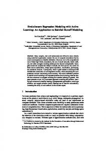
Figure 6

|

Comparison between measured and the predicted flows with NLP: verification.

for the maximum variance. SVM is now applied with the proposed new kernel, as defined in Equation (6). The best

RMSE of 0.304, resulting in an improvement of 58.75% in

performance on training data is obtained for C = 25 and

the verification data. The correlation coefficient also

s = 3. The study carried out in Islam et al. (2000) using

shows a significant improvement from 0.919 for NLP to

NLP is used for comparison with the results of the present

0.983 for SSA–SVM. It should be noted that the total

study.

number of training patterns used in SVM is significantly

Table 2 compares the prediction performance of the

lower than that in NLP. Figures 6 and 7 show the

single lead day forecasting on training and verification

comparison of measured and predicted flows for the veri-

data resulting from NLP and SVM methods. It can be seen

fication data resulting from NLP and SSA–SVM methods.

that data pre-processing with SSA coupled with SVM

The peak flow prediction is significantly improved

improves the prediction result significantly. While the

with the proposed technique. The low flows are also

RMSE as obtained by NLP is 0.736, SSA–SVM yields a

better predicted by the SSA–SVM approach by NLP.

150

C. Sivapragasam et al.

|

Rainfall and runoff forecasting with SSA–SVM approach

Journal of Hydroinformatics

|

03.3

|

2001

prediction accuracy of hydrologic variables than that of the non-linear prediction (NLP) method. SSA–SVM results in a significant improvement in the case study on Singapore rainfall prediction with a correlation coefficient of 0.70 as opposed to 0.51 obtained by NLP. Similarly, SSA–SVM yields 58.75% improvement (in terms of RMSE) over NLP in the runoff prediction for Tryggevælde catchment. Figure 7

|

Comparison between measured and the predicted flows with SSA–SVM: verification.

Moreover, the predictions from SVM offer special advantages as compared to other machine learning techniques like ANN. Unlike ANN, SVM does not require the architecture to be defined a priori. The structural risk minimization principle gives SVM the desirable property to generalize well in the unseen data. The dual representation offers the unique advantage of ease in dealing with the high-dimensional input vectors without loss of both generalization accuracy and computational efficiency. The optimization problem formulated for SVM is always uniquely solvable and, thus, does not suffer from the limitation of ways of regularization as in ANN, which may lead them to local minima.

ACKNOWLEDGEMENTS The authors wish to thank Mr Marco Sandri of Centro di Calcolo—C.I.C.A., Universita` di Verona, Italy for his constructive discussions on SSA. Also, the authors wish to express their sincere thanks to Danish Hydraulic Institute (DHI) and Meteorological Service Singapore for providing the daily runoff data of Tryggevælde catchment and Figure 8

|

Scatter plots of verification data for (a) NLP and (b) SSA–SVM.

Figure 8(a, b) show the scatter plots for the verification data with NLP and SSA–SVM, respectively.

Singapore rainfall data, respectively.

NOTATION The following symbols are used in this paper: R(b) = actual risk Remp(b) = empirical risk

CONCLUSIONS

V = confidence interval

In this study, it has been demonstrated that the proposed

h = VC dimension

approach, SSA–SVM, could yield significantly higher

x = input data

151

C. Sivapragasam et al.

|

Rainfall and runoff forecasting with SSA–SVM approach

Journal of Hydroinformatics

f = the non-linear mapping function

PC = Principal Components

f = the linear function in feature space

RC = Reconstructed Components

a and b = coefficients to be estimated

RBF = Radial Basis Function

d = measured targets

SOI = Southern Oscillation Index

x and x* = slack variables

SRM = Structural Risk Minimization

e = insensitive loss function

SSA = Singular Spectrum Analysis

a and a* = Lagrange multipliers

SVD = singular Value Decomposition

C = user specified constant,

SVM = Support Vector Machine.

|

03.3

|

2001

N = the number of training samples l = the number of support vectors K = the kernel function Knew = proposed kernel function [K1] = matrix obtained using kernel K1

REFERENCES

[K2] = matrix obtained using kernel K2

ASCE Task Committee. 2000a Artificial neural networks in hydrology-1: preliminary concepts. J. Hydrol. Engng 5(2), 115–123. ASCE Task Committee. 2000b Artificial neural networks in hydrology-2: hydrologic applications. J. Hydrol. Engng 5(2), 124–137. Babovic, V., Keijzer, M. & Bundzel, M. 2000 From global to local modelling: a case study in error correction of deterministic models. Hydroinformatics’2000, Iowa Institute of Hydraulic Research, Iowa, USA (CD-ROM). Cao, L. & Soofi, A. S. 1999 Nonlinear deterministic forecasting of daily dollar exchange rates. Int. J. Forecast. 15, 421–430. Cristianini, N. & Shawe-Taylor, J. 2000 An Introduction to Support Vector Machines. Cambridge University Press, Cambridge, UK. Dibike, Y. B. 2000 Machine learning paradigms for rainfall-runoff modelling. Hydroinformatics 2000, Iowa Institute of Hydraulic Research, Iowa, USA (CD-ROM). Drucker, H., Burges, C., Kaufman, L., Smola, A. & Vapnik, V. 1997 Support vector regression machines, Advances In Neural Information Processing Systems 9. MIT Press, Cambridge, MA, 156-161. Elsner, J. B. & Tsonis, A. A. 1997 Singular Spectrum Analysis: A New Tool in Time Series Analysis. Plenum Press, New York. Farmer, J. D. & Sidorowich, J. J. 1987 Predicting chaotic time series. Phys Rev. Lett. 59(8), 845–848. Grassberger, P. & Procaccia, I. 1983a Measuring the strangeness of strange attractors. Physica D 9, 189–208. Grassberger, P. & Procaccia, I. 1983b Characterisation of strange attractors. Phys. Rev. Lett. 50(5), 346–349. Gunn, S. R. 1997 Support vector machines for classification and regression. Technical Report. Image Speech and Intelligent Systems Research Group, University of Southampton. Haykin, S. 1999 Neural Networks: A Comprehensive Foundation. Prentice Hall International, Inc., New Jersey. Islam, N., Liong, S. Y., Phoon, K. K. & Liaw, C. Y. 2000 Forecasting of river flow data with general regression neural network. Accepted for publication in IAHS red book on International Symposium on Integrated Water Resources Management University of California, Davis.

s = width of the RBFs n = total number of events considered for prediction j = any vector∈Rn m = embedding dimension t = time delay X′ = trajectory matrix N′ = reduced training set after forming trajectory matrix L, R = left and right eigenvector matrix P = matrix of principal components p = individual principal component c = correlation dimension l = square root of variance CC = correlation coefficient RMSE = root mean square error.

Subscripts i, j, k = positive integer index m = measured s = simulated.

ABBREVATIONS The following abbreviations are used in this paper: ANN = Artificial Neural Network NLP = Non-Linear Prediction PCA = Principal Component analysis

152

C. Sivapragasam et al.

|

Rainfall and runoff forecasting with SSA–SVM approach

Jayawardena, A. W. & Lai, F. 1994 Analysis and prediction of chaos in rainfall and stream flow time series. J. Hydrol. 153, 23–52. Liong, S. Y. & Sivapragasam, C. 2000 Flood stage forecasting with SVM. Submitted for publication in J. Am. Water Res. Assoc. Lisi, F., Nicolis, O. & Sandri, M. 1995 Combining singular-spectrum analysis and neural networks for time series forecasting. Neural Processing Lett. 2(4), 6–10. Mukherjee, S., Osuna, E. & Girosi, F. 1997 Nonlinear prediction of chaotic time series using support vector machines. Neural Networks for Signal Processing—Proceedings of the IEEE Workshop. IEEE, Piscataway, NJ, pp. 511–520. Penland, C., Ghil M. & Weickmann, K. M. 1991 Adaptive filtering and maximum entropy spectra with application to changes in atmospheric angular momentum. J. Geophys. Res. 96, 659–671. Sharifi, M. B., Georgakakos, K. P. & Rodriguez-Iturbe, I. 1990 Evidence of deterministic chaos in the pulse of storm rainfall. J. Atmos. Sci. 47(7), 888–893. Smola, A. J. & Scholkopf, B. 1998 A tutorial on support vector regression. Technical Report NeuroCOLT Technical Report NC-TR-98-030, Royal Holloway College, University of London, UK.

Journal of Hydroinformatics

|

03.3

|

2001

Sivakumar, B., Liong, S. Y. & Liaw, C. Y. 1998 Evidence of chaotic behavior in Singapore rainfall. J Am. Water Res. Assoc. 34(2), 301–310. Sivapragasam, C. & Liong. S. Y. 2000 Improving higher lead period runoff forecasting accuracy: the SVM approach. 12th Congress of the Asia and Pacific Regional Division of the IAHR. Asian Institute of Technology, Bangkok, Vol 3, pp. 855–861. Takens, F. 1981 Detecting strange attractors in turbulence. In Dynamical Systems and Turbulence (ed. Rand, D.A. & Young, L.S.). Springer-Verlag, London, pp. 366–381. Theiler, J. 1987 Efficient algorithm for estimating the correlation dimension from a set of discrete points. Phys. Rev. A 36(9), 4456–4462. Vapnik, V. 1995 The Nature of Statistical Learning Theory. Springer-Verlag, New York. Vapnik, V. 1999 An overview of statistical learning theory. IEEE Trans. Neural Networks 10(5), 988–999. Vautard, R., Yiou, P. & Ghil, M. 1992 Singular-spectrum analysis: a toolkit for short, noisy and chaotic signals. Physica D 58, 95–126.