Right: An image similar to one of Damien Hirst's spot paintings. Abstract. Apparently-random distributions of colours in a discrete setting have been used by ...
Computational Aesthetics in Graphics, Visualization, and Imaging (2012) D. Cunningham and D. House (Editors)
Random Discrete Colour Sampling Henrik Lieng
Christian Richardt
Neil A. Dodgson
University of Cambridge
Figure 1: We present an algorithm that distributes colours randomly using a human-centric definition of randomness. Left: Colours distributed using Matlab’s random-number generator. Middle: Result of our algorithm. Notice that our algorithm does not produce any distinctive patterns. Right: An image similar to one of Damien Hirst’s spot paintings. Abstract Apparently-random distributions of colours in a discrete setting have been used by many artists and craftsmen in the past century. Manual colourisation is a tedious and difficult process. Automatic colourisation, on the other hand, tends not to not look ‘random’ to a human, as randomly-generated clusters and patterns stimulate human perception and break the appearance of randomness. We propose an algorithm that minimises these apparent patterns, making the distribution of colours look as if they have been distributed randomly by a human. We show that our approach is superior to current solutions, especially for small numbers of colours. Our algorithm is easily extendible to non-regular patterns in any coordinate system. Categories and Subject Descriptors (according to ACM CCS): I.3.8 [Computer Graphics]: Applications; I.3.m [Computer Graphics]: Miscellaneous—Visual Arts; J.5 [Arts and Humanities]: Fine Arts.
1. Introduction Abstract art is usually based on some object or complex structure that is simplified or abstracted. Of most relevance to this work is where coloured grids, dots, or regions are used by artists to flatten out the complexity of the real. As Rosalind Krauss put it, ‘in the spatial sense, the grid states the autonomy of the realm of art. Flattened, geometricised, ordered, it is antinatural, antimimetic, antireal. It is what art looks like when it turns its back to nature’ [Kra85]. c The Eurographics Association 2012.
Random colour sampling in the spatially discrete space was used in the early twentieth-century by numerous artists such as Jean Arp, Sophie Tauber and Vilmos Huszár. The grid represents order and structure; colourising the cells in this discrete spatial grid introduces randomness and chaos. The artist controls the amount of structure and chaos: the more regular the patterns, the more structure we get – and vice versa. A related type of art is the colour chart. Here, a small subset of the colour spectrum is laid out in either a struc-
H. Lieng et al. / Random Discrete Colour Sampling
tured fashion, like colour palettes in paint programs, or in a random fashion as shown in Figure 4. Gerhard Richter and Ellsworth Kelly are amongst the most prominent artists in this genre. A recent variation on this is Damien Hirst’s series of spot paintings. Random circles of colours with a fixed radius are distributed in some regular pattern. The colours are chosen ‘randomly’ by the artist. However, this is a human interpretation of randomness. Naïve machine simulations of Hirst’s work demonstrate clusters of spots of similar colours; Hirst’s actual paintings have no such clusters [Dod09]. A related problem, albeit in craft rather than art, is tiling a wall in a seemingly ‘random’ pattern with coloured tiles of a small number of colours. The Flickr group ‘Interesting Pixel Patterns’† collects photographs of such patterns of pixels or tiles on a regular grid. Looking at these photographs, we notice that ‘Tetris’-like clusters are deliberately avoided (unlike the left column of Figure 4). It is remarkably difficult to achieve a pattern that appears random to a human as humans are good at spotting patterns. True random selection of each tile’s colour therefore does not lead to an effective tiling; the selection must be moderated by a human. Our problem is thus that we wish to produce ‘random’ selections of colours that emulate what a human perceives as random, rather than a truly random distribution. Wei (2010) [Wei10] proposed algorithms for multi-class blue-noise sampling, that is, sampling using multiple classes of objects that are distributed in a blue-noise fashion, both within each individual class and between their unions. The algorithms can be applied to both continuous and discrete spaces. Our initial assumption was that, owing to their demonstrated success in the continuous space, these algorithms would serve to solve our problem. Unfortunately, the proposed algorithms are not suitable for discrete sampling using a small number of colours. Since they use a Euclidean distance metric, where adjacent horizontal and vertical cells are closer than diagonal adjacent cells, these algorithms tend to generate obvious diagonal lines of the same colour, Our algorithm, described in Section 3, takes an alternative approach. It picks an empty cell and computes an energy for each potential colour; the colour with the lowest energy is then chosen. Our energy function is based on a human-centric definition of randomness (Section 2). We show significant improvements over Wei’s blue noise algorithms (Section 4). The results produced by our algorithm include Hirst-like regular spot paintings (Figure 1), abstract colour charts (Figure 4), hexagonal grids (Figure 6), and non-regular dot patterns such as Fermat’s spiral (Figure 9). Our algorithm is
† http://www.flickr.com/groups/1302071@N22/
easily extendible to higher dimensions (see our supplementary video). Finally, we show that our algorithm is applicable to the problem of randomly tiling coloured tiles (Figure 7).
2. What do we mean by ‘random’? Randomness can be defined as ‘happening, done, or chosen by chance rather than according to a plan or pattern’ [Cam08]. For a colour distribution to appear ‘random’ to a human being it cannot contain any region with clearly visible patterns or clusters that deviate from the remainder of the distribution. These regions will attract the viewers attention and thus break the feel of randomness. Human visual perception is exceptionally well-trained to recognise patterns. Gestalt psychologists convincingly illustrate this through visual experiments. We can, for example, draw certain objects or shapes with just a few lines, and we will instantly recognise and visualise the complete outline of the object. Gestalt theorists argue that perceptual processes are dynamic rather than passive and the perceptual world is organised into patterns or configurations. The claim that ‘the whole is greater than the sum of its parts’ [Kof35] is an important tenet for the Gestalt psychologist. The Gestalt theorists argues that there must be a general underlying principle behind these phenomena. Wertheimer (1912) pioneered this notion with his ‘laws of grouping’ such as proximity, continuation and similarity [Wer12]. In this work, we focused on the proximity and similarity cues: dots that look similar and are close together are grouped together. This is clearly visible in Figure 1 (left) where horizontally adjacent similar cells ‘stick’ out. The ideas illustrated by Gestalt theory are used widely by artists. Due to the inherent complexity of the real world, it is impossible to capture it in its entirety. Artists must therefore provide simplified representations of the objects they depict. Arnheim (1956) provides an extensive review of this concept [Arn56]. Since humans are trained to identify patterns, these are expected in art. Hirst’s spot paintings, on the other hand, do not consist of any easily-identifiable patterns. We could therefore argue that these distributions look more random according to human perception than distributions made by a random-number generator. As Hirst’s works do not consist of any of the Gestalt groups, it is difficult to find interpretation other than ‘just random coloured dots’. One might hence argue they do not possess any æsthetic value. The art critic Peter Schjeldahl analyses Hirst’s spot paintings as follows: ‘. . . the pleasantly disorienting effects of colours that appear to be distributed at random: bright or muted and warm or cool, all ajumble. . . . His work comprehends all manner of things about previous art except, crucially, why it was created’ [Sch12]. However, we leave this argument to the philosopher. c 2012 The Author(s)
c 2012 The Eurographics Association and Blackwell Publishing Ltd.
H. Lieng et al. / Random Discrete Colour Sampling
Following our chosen Gestalt principles, we define randomness as the minimisation of certain features that are obvious to the human perceptual system: • regular patterns • clusters of the same colour • horizontal, vertical or diagonal runs of the same colour In a regular grid, where each cell has eight neighbours, producing a distribution that has no adjacent similar cells when sampling four colours or fewer is impossible. There must therefore be a balance between the various patterns. Also, longer patterns are more noticeable to human perception. These must hence be penalised more than smaller patterns. We also assume that vertical and horizontal patterns are more noticeable to the human perceptual system than diagonal patterns. This latter assumption is based upon informal experiments during the development of our algorithm. Our initial experiments revealed that we can identify all of the above features by looking only for straight-line runs of the same colour in the four principal directions (horizontal, vertical and the two diagonals). This obviously identifies such runs. It also identifies the strongest of the regular patterns, the checkerboard, through combination of the two diagonal directions through a given cell. And it also identifies clusters of the same colour by combinations of all four directions through a given cell.
• c p (c, x) is the count of a pattern p around location x for the colour c. If, for example, we are considering horizontal patterns (p = H) at the empty cell in the one-dimensional array [blue, red, empty, red, red, pink, red], and the current colour is c = red, the counter returns 3. Note that the counter stops when a different colour is encountered. The rightmost red is therefore not counted. • n controls the balance between square clusters and elongated patterns. A large n results in few elongated clusters but more square clusters. Conversely, a small n results in more similar adjacent cells in exchange for fewer square clusters. We use n = 5 for the results given in this paper. • ω p are weights for the various patterns. For example, large values of ωV and ωH , and small values of ωD1 and ωD2 result in more diagonal patterns but fewer vertical and horizontal patterns, which tends to produce a ‘checkerboard effect’. Figure 2 shows how these weights affect the results visually. ωH = ωV = 50, ωD{1,2}= 1
ωH = ωV = 1, ωD{1,2}= 50
3. Random discrete colour sampling Given a set of colours and a number of empty cells, our algorithm picks a random empty cell in each iteration and fills it with the colour of minimal energy (Equation 1). If there are multiple colours with the minimal energy, we pick one of these randomly. Note that we use a random-number generator when picking cells and colours randomly. The energy for each colour is based on cells of the same colour in the local neighbourhood. That is, we count nearby cells of the same colour that form linear runs, horizontally, vertically or diagonally where the linear runs align with the current cell. We compute an energy as follows: E(c, x) =
∑
ω p · c p (c, x)n ·
p∈{H,V,D1 ,D2 }
Pp + 1 , T +1
(1)
where c is the sample colour and x is the position of the current cell. The remaining terms of Equation 1 are: • H and V represent horizontal and vertical patterns, and D1 and D2 are diagonal patterns orientated like and , respectively. • Pp is the number of adjacent cells with similar colour in the direction defined by the pattern p. • T is the total number of adjacent cells with the same colour, that is T = PH + PV + PD1 + PD2 . c 2012 The Author(s)
c 2012 The Eurographics Association and Blackwell Publishing Ltd.
Figure 2: Effect of the weights ω p . Left: Higher weights for vertical and horizontal patterns produce diagonal patterns (i.e. checkerboard patterns). Right: Higher weights for diagonal patterns produce maze-like patterns.
3.1. Energy minimisation with sample control Even though we do not explicitly control the frequency of each colour, our tests show that we do get an even amount of each colour. Sometimes, however, we might want an exact number of samples for each colour. If we are tiling a kitchen for example, we usually only have a given number of each type of kitchen tile. We therefore extend our energy function by adding a weight, ωc for each colour. That is, we first compute the energy using Equation 1 and then normalise and scale this using the weight for the given colour: � � E(c, x) , (2) E 0 (c, x) = ωc · 1 − maxC E(C, x) where maxC E(C, x) is the colour with the highest energy, C is the set of all input colours, and ωc is updated in each iteration by nc ωc = 1 − , (3) nt (c)
H. Lieng et al. / Random Discrete Colour Sampling
where nc is the current count for the colour c and nt (c) is its target sample count, as specified by the user. The colour with the highest scaled energy, E 0 , is then picked.
we can sample in non-rectangular discrete spaces, and in any coordinate system. First, we redefine our energy function by accepting a set of searchable discrete patterns, Γ: E(c, x) =
3.2. Penalising similar colours Hirst’s spot paintings do not duplicate colours: every spot’s colour is unique. However, he uses colours that are very similar, which tend not to be adjacent. Hirst’s apprehension of randomness then, is the same as ours. To this end, we extend our energy minimisation algorithm to a continuous range of colours by penalising perceptually similar colours. This is particularly useful when sampling larger amounts of colours and we are bound to use similar-looking colours. We need to be able to measure perceptual similarities between colours. Using the RGB colour space for this is impractical as there are large correlations between the axes. Instead, we use the lαβ space [RCC98]. This is based on human perception where any change in the colour space corresponds to the same change in appearance. That is, the relative perceptual difference between two colours in lαβ space can be approximated using their Euclidean distance.
∑ ω p · c p (c, x)n ·
p∈Γ
Pp + 1 . T +1
(5)
A searchable pattern is defined by its forward and backward → − search directions, denoted by − s and ← s , respectively, which are lists of coordinates relative to a position x. For example, the 2D horizontal pattern H at x = (x, y) is defined as: � � −1 −2 · · · −x + 1 ← − s = (6) 0 0 ··· 0 � � 1 2 ··· m−x − → s = (7) 0 0 ··· 0 where m is the maximum x-coordinate in the 2D grid. In Section 4 we show numerous examples using this concept, such as sampling in the polar coordinate system, sampling using parametric functions, and sampling in 3D space-time. 4. Results
Similar colours are penalised by putting an additional weight between the colours when counting the patterns in the c p function of Equation 1. For this purpose, we use a colour similarity function, Ω(c1 , c2 ), based on the lαβ colour space. We embed this in the counter, c p , by adding difference between neighbouring colours to the current colour in the direction of the pattern p. Using the same example as before, where we are counting horizontal patterns in the empty cell in the array [blue, red, empty, red, red, pink, red], and the current colour of consideration is red, comparing with Ω might result colour similarities of [0, 1, _, 1, 1, 0.8, 1]. Then, the result of cH (red, empty) is: 1 + 1 + 1 + 0.8 + 1 = 4.8. Note that the counter still stops on a ‘different’ colour, that is when Ω(c1 , c2 ) = 0.
We compare the results of our new algorithm against Wei’s state-of-the-art ‘hard disk’ and ‘soft disk’ algorithms. For the results produced in this paper, we use Wei’s recommended relative radius of ρ ≥ 0.67 for the hard disk approach. For the soft disk results, we sample 50 samples in each iteration. The results produced using our algorithm have equal weights for all patterns (i.e. ω p = 1) and n = 5 for up to four colours. When sampling more than four colours, we observed that vertical and horizontal patterns are more noticeable than diagonal patterns, and therefore set ωH =ωV = 50, ωD1 = ωD2 = 1 and n = 2 to suppress them. All results are computed using square grids of 20 × 20 cells. The reported results are averaged over 100 runs for our and Wei’s hard disk algorithms, and 10 runs for the soft disk algorithm, as it is too slow to run 100 times.
We define the similarity of two colours c1 and c2 using their colour difference (as measured using the Euclidean distance kc1 − c2 k in lαβ space), which is then passed through a Gaussian function Gσ (x) = exp(−x2 /2σ2 ) to achieve a smooth falloff as colour distance increases. In addition, we truncate the colour similarity of colours that are sufficiently different. Specifically, we use ( Gσ (kc1 − c2 k) if kc1 − c2 k ≤ a Ω(c1 , c2 ) = (4) 0 otherwise
Figure 3 shows the performance in terms of minimising larger patterns. Here we see that our algorithm produces fewer adjacent cells of the same colour, a more balanced distribution between horizontal/vertical and diagonal patterns, and fewer large patterns than Wei’s techniques. The soft disk sampling algorithm produces more clusters than the other algorithms. This is very noticeable and thus breaks the feel of randomness. These differences are confirmed visually in Figure 4. Please refer to the supplementary material for more examples.
with values σ = 10 and a = 100 for the results in this paper.
The multi-dimensional nature of the statistical measures make evaluation challenging. We tackle this by computing a score for each given number of colours, defined by the average sum over the various counts for each pattern, where larger patterns are penalised:
3.3. Non-rectangular patterns Our original energy in Equation 1 assumes that the canvas is a rectangular grid, defined in a Cartesian frame. This simplification restricts us to only vertical, horizontal or diagonal patterns. We now generalise our concept of patterns such that
score =
1 · ∑ ∑ i · ci,p , |Γ| p∈Γ i
(8)
c 2012 The Author(s)
c 2012 The Eurographics Association and Blackwell Publishing Ltd.
H. Lieng et al. / Random Discrete Colour Sampling Horizontal & vertical patterns
Diagonal patterns
pseudo-random
our algorithm
Wei (2010)
1 0.1
2 colours
2 colours
10
Average count
100
1 0.1 0.01
4 colours
3 colours
10
Average count
100
3 colours
0.01
1 0.1 0.01 0
10 10 5 15 0 5 15 Number of adjacent cells with the same colour pseudo-random Wei’s soft disk
Wei’s hard disk our algorithm
Figure 3: Results of pattern analysis: each of the six graphs shows the number of patterns of consecutive same-colour cells observed for each length. In every cell, nearby cells for each considered pattern are counted using c p (c, x). Here, each pattern only searches in one direction, so that adjacent cells are not double-counted. Then, the total number of adjacent cells with the same colour is the sum of c p (c, x) for all cells x and patterns p. The columns compare different orientations of features and the rows show results for different numbers of colours. In almost all cases, our approach produces fewer patterns than the other techniques.
where i ∈ {2, 3, . . . } ranges over the possible lengths of patterns, and ci,p counts all instances of i same-colour adjacent cells within a pattern p. Figure 5 shows the results for this scheme for up to eight colours. Our algorithm consistently produces the best results, although Wei’s hard disk algorithm produces comparable results when sampling more colours. Table 1 compares run times on a computer with an Intel Quad 2.40 GHz CPU with 8 GB RAM. All algorithms are naïvely implemented in M ATLAB. Note that Wei’s algorithms can be sped up considerably using faster data strucc 2012 The Author(s)
c 2012 The Eurographics Association and Blackwell Publishing Ltd.
Figure 4: Colour chart created using random sampling, Wei’s hard disk algorithm and our algorithm for 2–4 colours. 1,000
Score
4 colours
10
Average count
100
pseudo-random Wei’s hard disk Wei’s soft disk our algorithm
500
0 2
3
4 5 6 Number of colours
7
8
Figure 5: Results using the score described by Equation 8.
tures [Wei10]. By looking at the algorithmic differences, however, our algorithm is bound to be faster. Wei’s hard disk algorithm uses a dart-throwing approach, which is relatively slow, like other rejection sampling approaches. Wei’s soft disk algorithm, on the other hand, appears to have a constant run time. This is because the run time depends only on the number of samples taken in each iteration and not the number of colours. Our algorithm on the other hand, is simple yet fast: it simply picks an empty cell and colours it with the ‘best’ colour. This results in a dramatic difference compared to the run times of the two other algorithms. Figure 1 shows coloured grids in the style of Damien
H. Lieng et al. / Random Discrete Colour Sampling
# colours
2
3
4
5
6
7
8
Hard disk
61
91
110
130
140
170
130
Soft disk
230
230
230
230
230
230
230
0.082
0.11
0.13
0.16
0.18
0.21
0.23
Ours
random distributions using just four colours, as shown in the example, is surprisingly hard. We encourage the reader to try this on a piece of paper. Most likely, some apparent patterns will stand out immediately. Standard kitchen tiles
Coloured kitchen tiles
Table 1: Run times of Wei’s soft and hard disk algorithms and our algorithm. All run times are given in seconds to two significant digits, computed on 20×20 grids and averaged over multiple runs.
Hirst’s spot paintings. Since we only use three colours in the middle picture, producing a randomly-looking distribution is not trivial. Using our definition of ‘randomness’, however, we get good results: there are no clusters of the same colour and no horizontal, vertical or diagonal patterns that ‘stick’ out. In the right picture of Figure 1, similar colours are penalised in lαβ space, and we observe that light colours are separated as they are deemed to ‘look’ similar. Using our generalisation, we can easily extend our Hirstlike plots to 3D (x, y,t). This is shown in the supplementary video. We add an additional pattern to our existing set of vertical, horizontal and diagonal patterns, which searches one step in time, both forward and backward: 0 0 ← − − → s = 0 and s = 0 . (9) −1 1 We set the weights for this pattern to 50, so that we most likely do not get two adjacent dots of the same colour at the same position between two time steps. The square grid, or tiling, used throughout this paper is one of the three regular tilings of the plane [GS86]. The other two are the triangular tiling and the hexagonal tiling. In Figure 6 we colour an hexagonal tiling by searching for patterns in 12 directions instead of 8, as in our square grid examples.
Figure 7: Coloured kitchen tiles using our algorithm. The original image (left) was recoloured with Adobe Photoshop using a colour chart created by our program as a template. In Figure 8 we plot points in the polar coordinate system. The patterns are defined similar to the patterns used in the regular Cartesian frame. That is, we search along the r and θ axis and two spiral-shaped directions (similar to the diagonal directions in the Cartesian frame). In Figure 9 we plot Fermat’s spiral using the golden angle (137.508◦ ) [Vog79], inspired by Hirst’s Valium. Both of these examples show the limitations of our algorithm. In the former example, we notice how we avoid patterns along the defined directions. Noticeable blocks of adjacent dots of the same colour are however produced as there are more potential patterns other than those four that are defined. The latter example is even harder as there are no obvious search directions. In Figure 9, we compare every fifth plotted point with each other as these might be grouped together. However, as we can see from the figure, it contains a fair amount of patterns, so this is not sufficient. Thus, further work on making the algorithm amenable to discretised continuous functions and sampling in the continuous space is needed. 5. Conclusion and Future Work
Figure 6: Colouring a hexagonal tiling using our algorithm (right) searching in 12 directions (left). Our random colour sampling approach can be applied to distributing coloured tiles, as shown in Figure 7. Creating
We present an algorithm for producing ‘random’ distributions of colours in a discrete space. By a ‘random’ distribution, we mean a distribution which minimises apparent patterns. We present, also, a human-centric measure of randomness. This human-centric definition of randomness is justified by the fact that the perceptual world is organised into patterns or configurations and not any particular mathematical notion which drives any random-number generator. Our algorithm is well suited for practical applications such as tiling kitchen tiles, as the designer is able to set the exact number of samples of each colour. Additionally, similar looking colours will not be grouped together when sampling from a larger set of colours. Finally, we show superior results compared to current solutions, both in terms of number of apparent patterns and run times. c 2012 The Author(s)
c 2012 The Eurographics Association and Blackwell Publishing Ltd.
H. Lieng et al. / Random Discrete Colour Sampling
tributions produced by our algorithm might not possess the blue-noise property. Extending our approach to a global optimisation is a promising direction for future work, as this would enable blue-noise constraints to be incorporated. Evaluating random discrete colour distributions quantitatively using our human-centric definition is justifiable since we can easily measure the number of apparent patterns of similar colours in a discrete grid. Our measure of success (the score of Equation 8), however, is rather similar to our energy function, and we can therefore expect that our algorithm performs better. Additionally, our take on randomness is based on Gestalt theory, which is a collection of observations about human perception; however, any attempt to formalise these hypotheses has been proven to be invalid [Hen84]. To this end, it would be interesting to carry out a qualitative study of the various approaches to distributing colours. Furthermore, this study could include extensions to our current definition of randomness to incorporate additional Gestalt cues, such as closure and past experience. Figure 8: Colour sampling in the polar coordinate system.
Acknowledgements ´ Thanks to Leszek Swirski and Tadas Baltrušaitis for providing useful comments. References [Arn56] A RNHEIM R.: Art and visual perception: a psychology of the creative eye. Faber and Faber, 1956. 2 [Cam08] C AMBRIDGE U NIVERSITY P RESS (Ed.): Cambridge Advanced Learner’s Dictionary. Cambridge University Press, 2008. 2 [Dod09] D ODGSON N. A.: Balancing the expected and the surprising in geometric patterns. Computers & Graphics 33, 4 (August 2009), 475–483. 2 [GS86] G RÜNBAUM B., S HEPHARD G. C.: Tilings and Patterns: An Introduction. W.H. Freeman & Company, 1986. 6 [Hen84] H ENLE M.: Isomorphism: Setting the record straight. Psychological Research 46 (1984), 317–327. 7 [Kof35] KOFFKA K.: Principles of Gestalt Psychology. Harcourt, 1935. 2 [Kra85] K RAUSS R. E.: The Originality of the Avant-Garde and Other Modernist Myths. The MIT Press, 1985. 1
Figure 9: Colour sampling using Fermat’s spiral.
[RCC98] RUDERMAN D. L., C RONIN T. W., C HIAO C.-C.: Statistics of cone responses to natural images: implications for visual coding. J. Opt. Soc. Am. A 15, 8 (Aug 1998), 2036–2045. 4
We use a random-number generator when selecting which cell to colourise. Even though we colour the chosen cell with the ‘best’ colour, we might end up with an unlucky ordering of cells, when we are forced to insert a colour which creates an avoidable long pattern. Using a more elaborate approach when picking cells, for example in a Poisson-disk manner, might produce fewer elongated patterns. Also, our energy minimisation is a local one and we might end up with an uneven distribution of colours globally. That is, the dis-
[Sch12] S CHJELDAHL P.: The Art World. Spot On. The New Yorker January 23 (2012), p. 84. 2
c 2012 The Author(s)
c 2012 The Eurographics Association and Blackwell Publishing Ltd.
[Vog79] VOGEL H.: A better way to construct the sunflower head. Mathematical Biosciences 44, 3–4 (June 1979), 179–189. 6 [Wei10] W EI L.-Y.: Multi-class blue noise sampling. ACM Transactions on Graphics 29, 4 (July 2010), 79:1–8. 2, 5 [Wer12] W ERTHEIMER M.: Experimentelle Studien über das Sehen von Bewegung. Zeitschrift für Psychologie und Physiologie der Sinnesorgane 61 (1912), 161–265. 2