Random Number Generators Founded on Signal and Information Theory

Random Number Generators Founded on Signal and Information Theory 1

David P. Maher and Robert J. Rance 1

2

2

Intertrust, Sunnyvale, CA, USA [email protected]

Lucent Technologies, Bell Laboratories Innovations, No. Andover, MA, USA [email protected]

Abstract. The strength of a cryptographic function depends on the amount of entropy in the cryptovariables that are used as keys. Using a large key length with a strong algorithm is false comfort if the amount of entropy in the key is small. Unfortunately the amount of entropy driving a cryptographic function is usually overestimated, as entropy is confused with much weaker correlation properties and the entropy source is difficult to analyze. Reliable, high speed, and low cost generation of non-deterministic, highly entropic bits is quite difficult with many pitfalls. Natural analog processes can provide nondeterministic sources, but practical implementations introduce various biases. Convenient wide-band natural signals are typically 5 to 6 orders of magnitude less in voltage than other co-resident digital signals such as clock signals that rob those noise sources of their entropy. To address these problems, we have developed new theory and we have invented and implemented some new techniques. Of particular interest are our applications of signal theory, digital filtering, and chaotic processes to the design of random number generators. Our goal has been to develop a theory that will allow us to evaluate the effectiveness of our entropy sources. To that end, we develop a Nyquist theory for entropy sources, and we prove a lower bound for the entropy produced by certain chaotic sources. We also demonstrate how chaotic sources can allow spurious narrow band sources to add entropy to a signal rather than subtract it. Armed with this theory, it is possible to build practical, low cost random number generators and use them with confidence.

Introduction RNGs (Random Number Generators) are hardware and/or software sources that supply bits (or numbers) that ideally are statistically independent. In this paper we will talk solely about analog RNGs, that is, RNGs whose initial source of entropy is analog noise. As such, these RNGs are non-deterministic. In contrast, PRNGs (pseudo-random number generators) are deterministic in that their output is completely determined from their initial state or “seed”. RNGs are used to generate independent bits for cryptographic applications such as key generation or random starting states, where it is vital that the key or state cannot Ç.K. Koç and C. Paar (Eds.): CHES'99, LNCS 1717, pp. 219-230, 1999. © Springer-Verlag Berlin Heidelberg 1999

220

D.P. Maher and R.J. Rance

be predicted or inferred by the adversary. They are also used as hashing or blinding factors in various signature schemes, such as the Digital Signature Standard. Our RNGs have employed either thermal or shot noise, and have been implemented in both discrete and integrated forms. Other RNGs have been driven by sources such as: vacuum tube shot noise, radioactive decay, neon lamp discharge, clock jitter, and PC hard drive fluctuations. We further define these RNGs as hybrid RNGs since they comprise an analog noise source followed by digital post-processing. The post-processing greatly enhances the entropy (statistical independence) of the output, usually at the cost of an acceptable reduction in bit-rate. The post-processing could also be termed digital nonlinear filtering or lossy compression. Finally, we further class the RNGs as either chaotic or non-chaotic. Reliable, high speed, and low cost analog random number generation of highly entropic bits is a hard problem. This is because practical noise sources are a few microvolts while other co-resident, typically fast-transitioning digital signals are several volts. Even greatly attenuated interference from these deterministic sources can rob the RNG output of most or all of the entropy that a cryptographic application may depend on. Amplification and sampling of noise signals can further degrade the entropy because the amplifiers are inevitably band-limited, and sampling thresholds are typically biased. By applying some results from chaotic processes and signal theory we have been able to overcome the problems mentioned above, producing reliable, high-speed, low-cost, highly entropic RNGs whose performance is supported by strong theory. In particular, we study the effect of filtering on sampled analog noise sources. We demonstrate that under ideal conditions, a relatively narrow-band noise source can be used to produce a perfectly uncorrelated bit-stream. Seeking more practical solutions, we demonstrate how simple digital feedback processes can be used to improve RNG statistics and to nullify the effects of certain spurious noise sources. Finally, we demonstrate how digital feedback, directly interacting with a chaotic amplifier, can produce a noise source that coerces other spurious noise sources to contribute their entropy to the main source, rather than rob that source of its entropy. We prove a lower bound for the amount of entropy per bit that such a chaotic source will produce, we calculate the probability density function for the source, and we discuss how to use this source to compress n bits of entropy into a vector of length n. We believe that the results provided here can help designers include high quality, stand-alone, non-deterministic RNGs in low-cost crypto-modules and ICs.

1 Signal Theory Applied to RNGs We begin by showing that it is possible to produce very good, random bit sequences of completely independent values by carefully filtering and sampling a non-white natural noise source. We show how bandwidth limitations reduce to bit-rate limitations. A classic natural random number generator is modeled as follows:

Random Number Generators Founded on Signal and Information Theory

WGN

n(t)

H

w(t)

C

S

221

x(t)

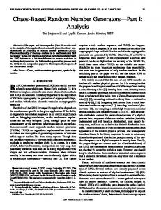
Fig. 1. Classic Random Number Generator

WGN is Stationary White Gaussian Noise that we assume is wide-band and lowpower (such as thermal or shot noise). H is the transfer function of a band-limited amplifier. C is a comparator or quantizer function, and S is a sampling process that samples every interval of length t. Generally one can find wide-band, low-power white noise sources, but to work with them considerable amplification is needed. An inevitable limitation of bandwidth results. The signal x(t) is expressed in terms of the Dirac delta function d(t): (1)

w(t)d(t - k t)

x(t ) = k

summing over all integers k. The Fourier Transform of x(t) is then X(f) = x(t)e -j2ptf dt = R

w(t)d (t - kt)e -j2ptf dt = R k

w(kt)e -j2pktf

(2)

k

Using the Poisson summation formula on the last expression, we get: X( f ) =

1 t

W(f - k / t)

(3)

k

For the moment, ignore the effect of the quantizer, and note that if the shape of W is completely determined by the filtering of the amplifier H, we can arrange that W(f) = 0 for |f| > 1/t by selecting the sampling rate to match the amplifier’s rolloff. In addition, if the amplifier characteristic is equalized so that W(t/2-f) = W(t/2+f), then the right hand side of Equation (3) is a constant, indicating white noise, and therefore x(t) will be completely uncorrelated. Again, if we ignore the effects of the quantizer, then by the Gaussian assumption we can conclude that the values x(nt) are independent. We have shown that we can apply the Nyquist rule of thumb: “Make the sampling rate about twice the bandwidth,” and we have shown that we can carefully filter a stationary Gaussian narrowband noise source to completely eliminate correlation. Nyquist theory refers to sampling theorems in hybrid analog and digital systems where the goal is to eliminate the effects of aliasing and to reduce intersymbol interference. We have shown that it applies just as well to sampled noise signals where the performance criterion is intersymbol correlation. It is also clear from the above analysis that if the original noise source is non-white, an equalizer W can be still be designed so that the sum in Equation (3) is constant. Recall that the effect of the quantizer has thus far been ignored. The theory is much more involved for most common quantizers. We will treat one common and useful case in the next section.

222

D.P. Maher and R.J. Rance

2 Practical and Simple Examples In order to economically manufacture a good natural random number generator, we have to use some simpler digital filtering techniques, shooting for less than Nyquist precision. We show how simple digital filtering and sampling techniques can reduce correlation. Some examples of RNGs with and without digital post-processing can be found in Murry [1], Bendat [2], Boyes [3], Castanie [4], and Morgan [5]. Referring to Figure 1, we assume w(t) has zero mean with a power spectral density function W (f), and we use a simple two-pole amplifier with non-Nyquist filtering. W (f) rolls off from a flat spectrum at f a and fb, the lower and upper cutoff frequencies of the amplifier. Let us also consider the effect of the quantizer function C. Here we assume that C is an infinite clipper. That is, C assigns the value +1 to a positive voltage and -1 to a negative voltage. We also assume the comparator has a bias with an offset voltage D. Let xn=x(nt). We are interested in values: mx = E[x n ] , The latter can be expressed in terms of rx ( i ) = E[x n x n+i ] . rw (t) = E[w(t) w(t + t)] . The mean of the process x is a straightforward error

function approximated by mx @ 0.4 D/s (when the offset is small enough compared to the signal power), and with the aid of Price’s theorem [6], the autocorrelation function can be expressed in closed form as: rw ( t) =

2 Sin -1 ( rn ( t)) +m p

(4)

2 x

where rn ( t) =

f b exp(- 2pf b t) - fa exp(- p 2 tfa fb - fa

)

(5)

For a typical selection of components for a low cost RNG as modeled above, we get unsatisfactory mean and correlation values even if we very carefully isolate the RNG components from spurious noise sources. Thus we are motivated to use some simple digital filtering techniques. First, suppose we follow the sampler in Figure 1 with a simple feedback loop, where the analog noise source below contains the sampler:

S’ ANALOG NOISE SOURCE

xn

yn

D Q

zn

D Fig. 2. Digital Processing

We note that if the delay D is one clock cycle then

. After a short period of

time, my is going to be extremely small even if the xi’s are highly biased and strongly

Random Number Generators Founded on Signal and Information Theory

223

correlated. This is clearly true when the xj are independent. More generally, we can

show that E[yi ] fi 0 almost as quickly as ( rx (1) + mx2 ) fi 0 , depending on the characteristics of w(t)’s autocorrelation function, rw (t) , which we assume is asymptotically well-behaved and monotonically decreasing (as in the case of the two pole filter we have assumed). The difficulty here is that the autocorrelation ry (1) = mx i/2

is unacceptable. Note that the effect of the feedback loop is just to shift values of lower order statistics to higher order statistics. Now consider the sequence zn. We sample the output wj at a rate fs’ = fs/r where fs is the sampling rate producing xk. Let the function D delay the feedback by d clock cycles, then E[zjzj-k] = E[(xrjxrj-dxrj-2d…)(xr(j-k)xr(j-k)-d…)]

(6)

We choose d to be relatively prime to r. Then when d does not divide k, we see that there are no duplications in the subscripts in the above expression, and so there are no symbolic cancellations of the x values, and so rz(k) is the expectation of the product of a large number of samples of x which grows larger as n grows large. As for the case when d divides k: If we set m=k/d, then E[zjzj-k] = E[yrjyr(j-k)] = E[xrjxrj-d … xrj-(rm-1)d]

(7)

Therefore, this correlation is the expectation of the product of rm bits each spaced d apart. This works very well with a decreasing autocorrelation function for w(t). In cases where the acf rw (t) decreases slowly, then the value of d. should be increased

to compensate. Heuristically, we are taking the expectation of the product of many –1 values spaced far apart in time. For a typical acf, increasing the spacing will effect an exponential reduction in expectation, and increasing the number of bits will also cause an exponential drop. Thus increasing d and r serve to reduce the expectation synergistically and powerfully. Both of these techniques are novel. With reasonable assumptions on n(t) and w(t), we can show that rz (1) £ Bn ( rx (1),m x2 ) given Bn : B n ( r, m 2 ) ”

ak ”

n/2 k =0

a k m n -2k r k

( )k!/ ((k/2)!p ) n/2 k

k/2

(8) (9)

The actual closed form expressions for rz (t) are difficult to analyze asymptotically. We use Price’s theorem [6] to calculate the autocorrelation function of the output of the infinite clipper, and our expressions include a determinant of an autocorrelation matrix whose entries are values of the autocorrelation function for the process n(t) at times nt (see Figure 1 again). For the example where n(t) is flat noise filtered by a two-pole filter the autocorrelation function magnitude, |rn(t)|, is eventually monotonically decreasing, and thus we can estimate bounds for rz(k). Overall, the key to improving the statistics is selection of the sampling rates S and S’ as we show next. Thus, we can produce a sequence zk with zero mean (after a brief transient), and unnoticeable correlation. In fact, the bound given above also provides a measure of independence in that |log(1 - E[x1x2…xrk])| bounds the average mutual information

224

D.P. Maher and R.J. Rance

between bits zi and zi+k. Thus, this system approximates a sequence of equiprobable mutually independent (Bernoulli) samples of events from a sample space {1, -1} which can be produced using simple components with very modest performance characteristics. Suppose we use a Western Electric WE-459G noise diode as the WGN source. It’s output is 0.8 mV/sqrt(Hz) with a power spectral density that is flat – 2 dB from 100 Hz to 500 kHz. We use a comparator with offset of D = 10 mV, and an amplifier with voltage gain of 100 and a flat transfer function from 100 Hz to 10 kHz. The mean will then be mx = 0.05. For a sampler S with frequency fs = 10 kHz, then the two-pole amplifier model above predicts all covariances between xi and xi+j for j between 1 and 50 to be on the -2 -3 order of 10 down to 10 . Applying the loop model, we “oversample” with fs = 30 kHz, and then set the second sampler frequency to fs’ = 10 kHz. Thus r=3, and we choose a delay of 256 bits. The output sequence zi then has zero mean, and all correlations are 0, 3m except rk(k)   (0.05) for k = 256m. In general, our experience shows that the above structure works extremely well under the assumption that we are reasonably faithful to the model, and we are careful to isolate the analog source from coupling effects from the digital filter components and other on-board components. This latter requirement is either difficult or expensive to satisfy, but it turns out that the same techniques mentioned above employing a double-loop topology will mitigate the effects of such coupling.

3 Reducing Coupling Effects by a Double Loop Measured statistics on the output of an implemented single-loop RNG showed a small mean bias. This result violated the above theory and we attributed this effect to coupling from the high-level digital output into the analog noise source. Coupling between the digital output and analog input is denoted by e. Since the digital output is 5 to 6 orders of magnitude larger than the analog noise levels, the coupling effect will be significant in practical designs and will place a bias on the yn, independent of the sub-sampling ratio. This places a fundamental upper limit on the output entropy. However, this limit can be surmounted by placing two loops in tandem:

ANALOG NOISE SOURCE

xn

yn D1

e2

S1

e1 D

Q

S2 un

zn

D

Q

vn

D2

Fig. 3. Double-Loop Coupling

The second loop exponentially mitigates the e1 coupling effect and that the first loop will similarly reduce the e2 coupling effect. In the first case, we can model the noise source and first loop as a single noise source with some mean bias induced by e1. The second loop will greatly enhance the bit independence as shown in the single-loop RNG analyses in the preceding sections. In the second case, the mean bias on the

Random Number Generators Founded on Signal and Information Theory

225

noise source output induced by e2 will just be treated as another noise source bias by the first loop. In fact, we have found that two loops are enough; three or more loops produce similar results. Again, this result is novel. No mean bias was observed at the output of a dual-loop RNG. We have implemented this dual-loop RNG in a single IC that includes fault-tolerance and testability features. The performance of this device bears out the theory.

4 Chaotic RNG This section departs from the above theory in that it treats a radically different type of RNG termed a chaotic RNG. Due to the great disparity between analog noise and digital signal levels, it is difficult (expensive) to ensure that interference of undesirable (low entropic) character will not dominate the analog noise source output. This dominance would nullify the beneficial effects of the various techniques described above. To free ourselves of this constraint, and other constraints imposed by other low-entropic interferers such as 1/f noise, we developed a chaotic RNG. The chaotic RNG has the advantageous property of accepting all noises, good and bad, and extracting their entropies. We discovered this idea by observing that the LSBs of high-resolution A/Ds tend to yield independent bits, regardless of the statistical nature and amplitude of the “desired” signal being converted. High resolution A/Ds require much hardware; this hardware can be sharply minimized by implementing the A/D in a loop with a 1-bit quantizer:

ANALOG NOISE SOURCE

ANALOG SUM

COMPARATOR RHP POLE

CLOCK

_ +

D

Q

OUTPUT BITS

Fig. 4. Chaotic RNG

The selection of the RHP (right-half-plane) pole and the clock frequency determine the loop gain, A, of the “A/D”. A standard, radix-2 A/D can be implemented by setting the loop gain at 2 and by setting the “analog noise source” to a fixed voltage. Setting A to unity and replacing the “fixed voltage” by a time-varying signal implements a sigma-delta modulator. Finally, increasing A to somewhere between 1 and 2, and replacing the “time varying signal” with an analog noise source creates a chaotic RNG. Electrical engineers are taught, almost from birth, to avoid poles in the right half plane. However, the loop’s negative feedback creates a stable overall response that

226

D.P. Maher and R.J. Rance

circumvents the RHP instability. We chose an RHP pole design since it provided the simplest implementation using discrete parts. In particular, the RHP pole comprises an OP-AMP (operational amplifier), capacitor, and a few resistors:

Vi

Rf

Ri C

+5

Rb

+ _

Vo

Rb Rb

Fig. 5. RHP Pole Circuit

Referring back to Figure 4, we can immediately draw up an equation describing the evolution of voltage at the OP-AMP’s output. We will call the normalized RHP pole output voltage, at sample time nT, bn . Note that this voltage at time (n+1)T is a linear combination of the voltage at time n, bn, the sign of the voltage at time n, sgn[bn], thermal noise, gn, and interference, sn . The first term is the initial state for the RHP filter, and the latter three terms are inputs accumulated by the RHP filter during the [nT, (n+1)T] period. The RHP pole will increase its initial state over this time period by a factor of A. After normalization, the voltage is described as bn +1 = Ab n - sgn[b n ]+ g n + s n

(10)

For convenience, we will often use cn as shorthand for sgn[bn] . 4.1 What Is Chaos? Chaos can be described as a response that grows exponentially larger with time due to an arbitrarily small perturbation. A good introductory description to chaos is Schuster [7]. Note that its title is “Deterministic Chaos”. In fact, it is the marriage of (analog) deterministic chaos with an analog noise source that engenders a potent random number generator. Mathematically, a positive Lyapunov exponent defines chaos. In discrete time, the Lyapunov exponent is defined as the averaged logarithm of the absolute value of gain each cycle. For our chaotic RNG, the gain A is constant, so the Lyapunov exponent is ln(A) . Since A > 1 , the exponent is positive, verifying chaos.

Random Number Generators Founded on Signal and Information Theory

227

4.2 Other Chaotic RNGs Bernstein [8] and Espejo-Meana [9] describe two (of many) possible implementations of chaotic RNGs. Of the two, Espejo-Meana is the most similar to the implementation described here. 4.3 Why Is Chaos Good for Random Number Generation? Chaos guarantees that any noise contribution, no matter how small and how buried in deterministic interference, will ultimately significantly effect the output bits since the noise’s effect increases exponentially. This means that we can greatly relax the isolation requirements on the analog noise source. As long as the deterministic or low-entropic interference does not lower the Lyapunov exponent by causing OP-AMP saturation, chaotic operation will occur. In fact, we built the above circuit with both analog and digital circuitry powered by the same +5V supply (which also powered much other digital circuitry). We observed no interference with chaotic operation. This RNG employs the simplest possible topology for a chaotic RNG implemented in discretes, has a constant Lyapunov exponent, and is therefore (relatively) easily analyzed. In Appendix A, we calculate a lower bound on the output bit entropy, expressed in bits: Hlb = ( N - 1) log 2 ( A) -

1 log 2 1- A -2 + 2

(

)

( )

log 2 s g +

177 .

(11)

Here N denotes the number of successive output bits collected and sg denotes the noise standard deviation. Note that for large N,

H lb » N log 2 ( A)

(12)

We have implemented this chaotic RNG and have verified that its output entropy approximates this lower bound to the precision we could measure. The output entropy is guaranteed in the sense that it will always be greater than the bound expressed in Equation 11, independent of any non-saturating interfering signal. This is a very important property for an RNG. In contrast, typical non-chaotic designs are plagued with very difficult isolation issues, tight tolerance on parameter matches, or clock phase-locking. Chaotic designs are often plagued with regions with negative Lyapunov exponents. Finally, both chaotic and non-chaotic designs can often be very difficult to analyze. 4.4 Output Whitening The derivation in Appendix A suggests a particular form of post-processing to provide independence. Specifically, we proved that the two sides of Equation 13 are asymptotically equal: N -1 k=0

A- k c k »

N -1 k=0

A- k g k +

N -1 k=0

A- k sk

(13)

228

D.P. Maher and R.J. Rance

where ck = sgn[bk] and the sk denote the interfering signal(s). The LHS comprises a quantizer that represents accurately a Gaussian random variable with some mean arising from the interference. The post-processor can then re-express the LHS as a binary number, which will comprise a standard binary-weighted A/D converter. Selecting a (large) subset of the bits of this binary number will yield a nearly independent bit-stream. Heuristically, the MSBs are not independent since they are heavily influenced by the signal’s distribution. Also, the LSBs after some point cannot convey any additional entropy, since only N log2(A) bits of entropy are available. Thus at this point, these LSBs become deterministically related to the prior bits. This leaves us with a mid-range of bits that are independent. Of course other whitening methods such as post-processing via a hash function or DES are always valid. 4.5 Concluding Remarks on Chaotic RNG We believe that the following are novel with regard to this type of chaotic RNG: use and implementation of RHP pole, calculation of entropy lower bound, realization that this lower bound is independent of external interference, form of whitening filter, and the derivation of a probability distribution.

References [1] H. F. Murry, “A General Approach for Generating Natural Random Variables,” IEEE Trans. Computers, Vol. C-19, pp. 1210-1213, December 1970. [2] J. S. Bendat, Principles and Applications of Random Noise Theory, John Wiley and Sons, Inc., 1958. [3] J. D. Boyes, “Binary Noise Sources Incorporating Modulo-N Dividers,” IEEE Trans. Computers, Vol. C-23, pp. 550-552, May 1974. [4] F. Castanie, “Generation of Random Bits with Accurate and Reproducible Statistical Properties,” Proc. IEEE, Vol. 66, pp. 807-809, July 1978. [5] D. R. Morgan, "Analysis of Digital Random Numbers Generated from Serial Samples of Correlated Gaussian Noise", IEEE Trans. on Info. Theory, Vol. IT-27, No. 2, March 1981, pp. 235-239. [6] R. Price, “A Useful Theorem for Non-linear Devices Having Gaussian Inputs,” IRE PGIT, Vol. IT-4, 1958. [7] H. G. Schuster, Deterministic Chaos, VCH, 1989. [8] G. M. Bernstein, M. A. Lieberman, "Secure Random Number Generation Using Chaotic Circuits", IEEE Trans. on Circuits and Systems, Vol. 37, No. 9, September 1990, pp. 11571164. [9] S. Espejo-Meana, J. D. Martin-Gomez, A. Rodriguez-Vazquez, J. Huertas, "Application of Piecewise-Linear Switched Capacitor Circuits for Random Number Generation", Proc. Midwest Symp. Circuits and Systems, August 1989, pp. 960-963.

Random Number Generators Founded on Signal and Information Theory

Appendix:

229

Entropy Calculation

Equation (10) is cast into an equivalent form by applying the filter

N -1

A- k ( ) :

k =0

A-( N -1) bN = Ab0 +

N -1 k=0

(14)

A- k ( g k + s k - c k )

Due to the negative feedback via the {cn}, |bn| < 1 for all n. Thus the RHS above is -(N-1) -(N-1) bounded in amplitude by A . In other words, with maximum error A , N -1 k =0

A - k c k » Ab 0 +

N -1 k=0

A-k s k +

N -1 k =0

For fixed N, the RHS of Equation (A2) is the sum of: 1. The initial condition, Ab0 2. A possibly large term due to the extraneous interference called S: 3.

A zero-mean Gaussian random variable:

(15)

A-k gk

S”

N -1 k=0

G”

N -1 k= 0

A -k s k

A-k gk

We cannot rely on Ab0 and S to supply entropy, at least entropy that is unknown to an adversary who is attempting to break a cryptosystem. The initial condition b0 may be largely deterministic if it is defined as the initial value of bn just after the circuitry has been powered-up or supplied with a clock. Moreover, b0 may be correlated to the previous exercise of the RNG, thereby reducing its entropy. Since we cannot specify what entropy that S will have that is unknown to the adversary, we will assume conservatively that S is deterministic. Therefore, for the remainder of this argument, we conservatively model the RHS of Equation (15) as a Gaussian random variable with mean (Ab0 + S) and standard deviation

sG ”

sg

(16)

1 - A-2

The LHS of Equation (15) is the (scaled) quantized value of the RHS in the sense that the {ck} assume values of {-1,1} which can be mapped into binary ones and zeros. The quantizer defined by the set {ck} has the property that it represents the -(N-1) RHS of this equation with a maximum error of A . There is an infinite set of quantizers that have this same property. Generally, these quantizers would have different entropies. The minimum-entropy quantizer with this property is one with as few quantization steps as possible, namely one that uniformly spans [-1, +1] with step -(N-1) size 2A . The entropy of this minimum-entropy quantizer is thus a lower bound on entropy of the {ck} quantizer. We calculate this lower bound here: Divide the [-1, +1] range into 2M levels, M positive and M negative. Then, to a high accuracy since M is very large, M»

AN -1 2

(17)

230

D.P. Maher and R.J. Rance

The entropy (in nats) of this quantizer is

( )

Hnats = -2

M i=1

( )

2

(18)

2

i-i i-i exp - 2 2 exp - 2 2 2s G M 2s G M Ł ł Ł ł ln 2p s G M 2p s G M Ł

ł

i denotes the mean value of the RHS of Equation (A2): i ” ( Ab0 + S ) M . The tails of

the Gaussian pdf have been ignored since sG is small. Expanding the natural logarithm in Equation (18) gives (19)

( )

2

H nats = 2

M i =1

i -i exp - 2 2 Ł 2s G M ł Ø Œ ln( M ) + ln Œ 2p s G M º

(

)

(i - i)

ø œ 2s M œ ß 2

2p s G +

2 G

2

The first two terms in the brackets are independent of i and equivalently pre-multiply the summation operator. The weighting function, exp(¼) is just a pdf which sums to one1. The last term in the brackets, when summed, very closely approximates the following integral where x ” i = Ab + S : 0

M

2

1

0

( x - x) exp 2s

Ł

2 G

2p s G

(20)

2

(

)

2

ł x-x dx 2s 2G Ł ł

The integral approximates unity due to the small sG. Therefore, the entropy is Hnats = ln( M) + ln

(

)

(21)

2p s G + 1

Substituting for sG and M from Equations (16) and (17), and converting to bits yields H lb = ( N - 1) log 2 ( A) -

1

1 log 2 1- A-2 + 2

(

)

Again ignoring the tails of the Gaussian since sG is small

( )

log 2 s g +

177 .

(22)