Range-Free Localization Scheme in Wireless Sensor Networks Based ...

Hindawi Publishing Corporation International Journal of Distributed Sensor Networks Volume 2013, Article ID 620248, 10 pages http://dx.doi.org/10.1155/2013/620248

Research Article Range-Free Localization Scheme in Wireless Sensor Networks Based on Bilateration Chi-Chang Chen, Chi-Yu Chang, and Yan-Nong Li Department of Information Engineering, I-Shou University, Kaohsiung 84001, Taiwan Correspondence should be addressed to Chi-Chang Chen; [email protected] Received 4 October 2012; Accepted 17 December 2012 Academic Editor: Long Cheng Copyright © 2013 Chi-Chang Chen et al. is is an open access article distributed under the Creative Commons Attribution License, which permits unrestricted use, distribution, and reproduction in any medium, provided the original work is properly cited. A low-cost yet effective localization scheme for wireless sensor networks (WSNs) is presented in this study. e proposed scheme uses only two anchor nodes and uses bilateration to estimate the coordinates of unknown nodes. Many localization algorithms for WSNs require the installation of extra components, such as a GPS, ultrasonic transceiver, and unidirectional antenna, to sensors. e proposed localization scheme is range-free (i.e., not demanding any extra devices for the sensors). In this scheme, two anchor nodes are installed at the bottom-le corner (Sink X) and the bottom-right corner (Sink Y) of a square monitored region of the WSN. Sensors are identi�ed with the same minimum hop counts pair to Sink X and Sink Y to form a zone, and the estimated location of each unknown sensor is adjusted according to its relative position in the zone. is study compares the proposed scheme with the well-known DV-Hop method. Simulation results show that the proposed scheme outperforms the DV-Hop method in localization accuracy, communication cost, and computational complexity.

1. Introduction Wireless sensor networks (WSNs) have gained worldwide attention in recent years. A WSN consists of spatially distributed autonomous sensors that cooperatively monitor a deployed region for physical or environmental conditions, such as temperature, sound, vibration, pressure, motion, and pollutants. e manufacturing of small and energy efficient sensors has become technically and economically feasible because of recent advances in microelectromechanical systems (MEMSs) technology. A sensor node can sense, measure, and gather information from the environment and, based on some local decision process, transmit the sensed data to sinks (or base stations) through a wireless medium. e transmission power consumed by a wireless radio is proportional to the distance squared or even a higher order in the presence of obstacles. us, multihop routing is usually considered for sending collected data to the sink instead of direct communication. Most WSN routing algorithms require the position information of sensor nodes. However, for some hazardous sensing environments, it is difficult to

deploy the sensor nodes to the required locations. us, for environments in which it is difficult to plan the location of sensors in advance, localization techniques can be used to estimate sensor positions. e simplest and most common localization technique is to install a GPS receiver on each sensor in the sensor networks. Although the cost of GPS receivers is falling, they are still too costly, in price and energy consumption, to install in a sensor network. is study proposes a low-cost yet effective WSN localization scheme. is scheme needs only two anchor nodes and uses low-complexity operations to estimate the location of unknown nodes. is study also compares the performance of the proposed scheme with the DV-Hop [1] method to show its superiority. e rest of this paper is organized as follows. Section 2 reviews related research on WSN localization algorithms. Section 3 presents the communication protocol used to divide the deployed region into zones and the preliminary localization method. Section 4 introduces the more accurate enhanced method to estimate the positions of the unknown sensor nodes. Section 5 provides a simulation of the proposed localization scheme and a comparison of its performance

2

International Journal of Distributed Sensor Networks

with the DV-Hop method. Finally, Section 6 offers a conclusion.

2. Related Work Research interest in WSN localization has increased greatly in recent years. Traditional WSN localization technologies can be divided into two categories: range-based methods and range-free methods [2]. A range-based method positions the sensor nodes using additional devices, such as timers, signal strength receivers, directional antennas, and antenna arrays. In contrast, a range-free method requires no additional hardware and instead uses the properties of the wireless sensor network and the appropriate algorithms to obtain location information. Range-based localization relies on the availability of point-to-point distance or angle information. e distance/angle information can be obtained by measuring time of arrival (ToA) [3], time difference of arrival (TDoA) [4], received signal strength indicator (RSSI) [4], and angle of arrival (AoA) [5]. Range-based localization may produce �ne-grained resolution but places strict requirements on signal measurements and time synchronization. Range-free localization requires no distance or angle measurements among nodes. is technique can be further divided into two categories: local techniques and hopcounting techniques [2]. In the local techniques, a node with unknown coordinates collects the position information of its neighbor beacon nodes with known coordinates to estimate its own coordinate. In the simple centroid algorithm proposed in [6], each sensor estimates its position as the centroid of the locations of the neighboring beacons. A density-adaptive algorithm can reduce the number of computation errors if beacons are well positioned [7]. However, this is unfeasible for ad hoc deployment. Later, He et al. proposed the APIT method [8], which divides the environment into triangular regions between beacon nodes. Each sensor determines its relative position based on the triangles and estimates its own location as the center of gravity of the intersection of all the triangles that the node may reside in. However, APIT requires long-range beacon stations and expensive highpower transmitters. A hop-counting technique, called DV-Hop method, was proposed by Niculescu and Nath in [1]. In the DV-Hop method, each unknown node asks its neighboring beacon nodes to provide their estimated hop sizes and then attempts to obtain the smallest hop count to its neighbor beacon nodes using the designated routing protocol. Each unknown node estimates the distances to its neighbor beacon nodes by the hop counts to them and the hop size of the closest beacon node. e unknown nodes then apply trilateration to estimate their position based on the estimated distances to three suitable neighbor beacon nodes. ere are many followup studies of the DV-Hop method. e authors of [9] proposed the DV-Loc method, which shows how Voronoi diagrams can be used efficiently to scale a DV-Hop algorithm while maintaining or reducing the DVHop localization error. e main concept of the DV-Loc

C B

A

Sink X

Sink Y

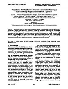
F 1: A scenario of 300 sensors with a communication range of 20 m, with the monitored region (200 × 200 m2 ) divided into zones. e colored irregular arcs are added to facilitate visualization of the zones.

Sink CR

F 2: A scenario of maximum distance to the sink: sensor nodes are located at the edge of the communication range. us, the maximum distance of sensors from the sink with hop count 𝑛𝑛 is 𝑛𝑛 𝑛 CR, where CR is the communication range.

method is to use a Voronoi diagram to limit the scope of the �ooding in a DV-Hop localization system. DV-Loc is a scalable solution that uses the Voronoi cell of a node to limit the region that is �ooded when computing its position to reduce its localization error. e authors of [10] proposed a range-free localization algorithm that uses expected hop progress to predict the location of WSN sensors. e algorithm is based on an analysis of hop progress in a WSN with randomly deployed

International Journal of Distributed Sensor Networks

D C

B A

Sink CR

F 3: A scenario of minimum distance to the sink: sensor nodes are two in a group located close to the edge of the communication range.

3 a node’s relative position than an integer-valued hop count. In that paper, the author presented an algorithm termed HCQ (hop-count quantization) to perform this transformation. Bilateration [12, 13], which is derived from multilateration, is based on the distance differences from an unknown node to two beacons at known locations. Unlike multilateration, which usually uses an iterative method to estimate the location of an unknown node, bilateration uses a basic geometry property, the intersection of two circles, to calculate the location of an unknown node. e computation of bilateration is much simpler than that of multilateration, which usually applies more expensive computation such as the least squares method. e disadvantage of bilateration is that the error rate is sensitive to the distance estimation to the beacon nodes. In [12], Cota-Ruiz et al. presented a distributed and formula-based bilateration algorithm that can be used to provide an initial set of locations. In their scheme, each node uses distance estimates to beacons to solve a set of circlecircle intersection (CCI) problems, solved through a purely geometric formulation. e resulting CCIs are processed to pick those that cluster together, and the average is then used to estimate an initial node location. A similar bilateration algorithm was also proposed by the authors in [13] independently.

3. Zone-Based Localization Scheme

No. 4 sensor

No. 1 sensor No. 2 sensor

No. 5 sensor No. 3 sensor

F 4: A scenario aer broadcasting step. Sensor No. 5 is located at the southwest corner.

sensors and arbitrary node density. By deriving the expected hop progress from a network model for WSNs regarding network parameters, this system can compute the distance between any pair of sensors. Traditionally, hop counts between any pair of nodes can only take an integer value, regardless of the relative positions of nodes in the hop. e authors of [11] argued that partitioning a node’s one-hop neighbor set into three disjoint subsets according to their hop-count values can transform the integer hop count into a real number. e transformed real number hop count is then a more accurate representation of

As mentioned in Section 1, some WSNs encounter difficulty in planning the location of sensors in advance. However, most routing algorithms require the information of sensor location. is section presents the proposed localization scheme to estimate the location of sensors. e following section extends the scheme to obtain a more accurate estimation of sensor locations. e basic communication protocol used in the proposed scheme is �ooding, which is a simple and effective mechanism for sending messages between sinks and sensor nodes. Flooding guarantees that sinks can reach any target node as long as the network is connective. In this scheme, the �ooding mechanism serves as the initial routing step to acquire the minimum hop count to each sink for each sensor. 3.1. Localization Scheme. In the proposed localization scheme, called the zone-based localization method (ZBLM), two sink nodes are installed at the lower-le corner (Sink X) and the lower-right corner (Sink Y) of a square monitored region (Figure 1). is scheme assumes that (1) all the sensors are homogeneous, (2) they are uniformly deployed, and (3) the network is connective. e ZBLM consists of three major steps: compute minimum hop counts, divide the monitored region into zones, and assign the coordinate of sensors for each zone. Step 1 (Compute Minimum Hop Counts). First, we allow both Sink X and Sink Y to broadcast a hop-counting packet (HC packet in short) to their neighbor sensors. e HC packet contains two �elds: (1) Min_hc (minimum hop count

4

International Journal of Distributed Sensor Networks

to the source node), initialized to 0 and (2) the source node ID (0 for Sink X and 1 for Sink Y). Each sensor records two current minimum hop count values (say, 𝑋𝑋hop and 𝑌𝑌hop ) to Sink X and Sink Y, respectively, which are both set to positive in�nity initially. Once a sensor receives an HC packet, it checks the hop count �eld Min_hc in the HC packet. If Min_hc + 1 is smaller than its corresponding current minimum hop count value 𝑋𝑋hop (or 𝑌𝑌hop ), then it increases Min_hc by one before forwarding the packet to its neighbors and updates its 𝑋𝑋hop (or 𝑌𝑌hop ) to the new Min_hc value accordingly. Otherwise, the sensor discards the current incoming HC packet. Step 2 (Divide the Monitored Region into Zones). Aer �nishing the �ooding of HC packets by Step 1, each sensor should have two minimum hop-count values (𝑋𝑋hop , 𝑌𝑌hop ) for Sink X and Sink Y, respectively. Sensors with the same (𝑋𝑋hop , 𝑌𝑌hop ) pair are in the same zone (note that the following subsection claims that the zone tends to be a geometry quadrilateral), and it is denoted as zone (𝑋𝑋hop , 𝑌𝑌hop ). Figure 1 shows a scenario of dividing the monitored region into zones, in which the color irregular arcs are added for ease of visualization. In this �gure, each node has its own (𝑋𝑋hop , 𝑌𝑌hop ) pair. For example, 𝑋𝑋hop of Node A is 3 and 𝑋𝑋hop is 8. erefore, Node A is in zone (3, 8). Similarly, Node B is in zone (6, 5), and Node C is in zone (5, 7). Step 3 (Assign the Coordinate of Sensors for Each Zone). Although we have the hop counts of each sensor and, therefore, know which zone a sensor belongs to, this information is still insufficient for identifying the location of a given sensor. As shown in Figure 1, the distance of each hop is not necessarily the same, and thus the band width corresponding to a hop is not necessarily equal to the communication range. e next subsection analyzes the range of the distance to the sinks for a given sensor node with its minimum hop count values and gives the estimated distance to the sinks. e current subsection assumes that we already have the estimated distances to Sink X and Sink Y for each node. Suppose that the coordinates of Sink X and Sink Y are (0, 0) and (𝑤𝑤𝑤𝑤), respectively, where 𝑤𝑤 is the length of the square monitored region. Denote the distances from an unknown sensor S to Sink X and to Sink Y as 𝑑𝑑𝑥𝑥 and 𝑑𝑑𝑦𝑦 , respectively. e coordinate (𝑥𝑥𝑥𝑥𝑥) of Sensor S is the intersection of two circles centered at (0, 0) and (𝑤𝑤𝑤𝑤), respectively. erefore, (𝑥𝑥𝑥𝑥𝑥) can be obtained using the following equations: 2

(𝑥𝑥 𝑥 𝑥)2 + 󶀡󶀡𝑦𝑦 𝑦𝑦󶀱󶀱 = 𝑑𝑑2𝑥𝑥 ,

(1)

2

(𝑥𝑥 𝑥 𝑥𝑥)2 + 󶀡󶀡𝑦𝑦 𝑦𝑦󶀱󶀱 = 𝑑𝑑2𝑦𝑦 .

us, 𝑥𝑥 𝑥𝑥𝑥𝑥2𝑥𝑥 − 𝑑𝑑2𝑦𝑦 + 𝑤𝑤2 )/2𝑤𝑤 and 𝑦𝑦 𝑦 𝑦󵀆󵀆𝑑𝑑2𝑥𝑥 − 𝑥𝑥2 . Because sinks are installed at the lower le and lower right corners of the monitored region, we can only take the positive solution of y. erefore, the coordinate of the unknown sensor S is 󶀪󶀪

𝑑𝑑2𝑥𝑥 − 𝑑𝑑2𝑦𝑦 + 𝑤𝑤2 2𝑤𝑤

, 󵀎󵀎𝑑𝑑2𝑥𝑥

− 󶀧󶀧

𝑑𝑑2𝑥𝑥 − 𝑑𝑑2𝑦𝑦 + 𝑤𝑤2 2𝑤𝑤

2

󶀷󶀷 󶀺󶀺 .

(2)

For (1) to produce a real solution, the sum of 𝑑𝑑𝑥𝑥 and 𝑑𝑑𝑦𝑦 (the radii of two circles) must be greater than or equal to w (the distance between two centers). is constraint is considered when estimating the distances 𝑑𝑑𝑥𝑥 and 𝑑𝑑𝑦𝑦 .

3.2. Estimate the Hop Distances between Sensors and the Sinks. At �rst, we claim that sensors with the same (𝑋𝑋hop , 𝑌𝑌hop ) pair tend to congregate in a quadrilateral. Suppose the length of the square monitored region is m, the communication range of each sensor is CR, and the total number of nodes is 𝑛𝑛. e probability that a node 𝑣𝑣 is within the communication range of another given node 𝑢𝑢 is (𝜋𝜋 𝜋 CR2 )/𝑚𝑚2 . Since the total number of nodes is n, the expected number of neighbor nodes, say 𝜌𝜌, for 𝑢𝑢 is (𝑛𝑛𝑛𝑛𝑛𝑛𝑛𝑛𝑛𝑛 CR2 )/𝑚𝑚2 ). For example, if 𝑚𝑚 𝑚𝑚𝑚𝑚, CR = 30, and 𝑛𝑛 𝑛𝑛𝑛𝑛, then 𝜌𝜌 𝜌𝜌𝜌𝜌𝜌𝜌𝜌𝜌𝜌𝜌𝜌𝜌𝜌𝜌𝜌 𝜌𝜌𝜌2 )/2002 ) ≅ 21. Previous research [14] provided a more precise estimation of node degree that considers the border effect. According to [14], 𝜌𝜌 𝜌𝜌𝜌𝜌𝜌𝜌𝜌𝜌𝜌𝜌𝜌𝜌2 −(8/3)𝑟𝑟3 +((11/3)−𝜋𝜋𝜋𝜋𝜋4 ), where 𝑟𝑟𝑟𝑟CR/𝑚𝑚𝑚. erefore, 𝜌𝜌 𝜌𝜌𝜌 for this case. According to [15], message forwarding between any two nodes through �ooding occurs along the straight-line path with a probability greater than 0.85 if the number of neighbor nodes is greater than or equal to 15. According to the previous paragraph, if CR = 20, then 𝜌𝜌 is greater than 15 as long as 𝑛𝑛 𝑛 𝑛𝑛𝑛. Alternatively, if CR = 30, then 𝜌𝜌 is greater than 15 as long as 𝑛𝑛 𝑛 𝑛𝑛𝑛. us, if both the forwarding paths from Sink X and Sink Y progress along straight lines, then the sensors with the same (𝑋𝑋hop , 𝑌𝑌hop ) pair tend to congregate and form a quadrilateral (called a “zone” in this paper). e experiment in this study shows that the “zone effect” still exists for the case CR = 20 and 𝑛𝑛 𝑛𝑛𝑛𝑛 (𝜌𝜌 𝜌 𝜌) (Figure 1). e following discussion presents two extreme cases in which the message is forwarded along the straight line. e hop distance between sensors is related to the communication range and the density of the sensors in the region [14, 15]. For high density, each sensor has a certain number of sensors within its communication range. erefore, for Sink X (or Sink Y), it is highly possible that sensors are located at the edge of the communication range. For the extreme case shown in Figure 2, sensor nodes always exist at the edge of the communication range of each hop from the sink. erefore, assuming that the communication range is CR, the maximum distance of a sensor with hop count 𝑛𝑛 from the sink is 𝑛𝑛 𝑛 CR. e other extreme case occurs when the density of sensor nodes in the region is low and each sensor node has few neighbors, yet the network remains connective. As Figure 3 shows, sensor nodes are two in a group located close to the edge of the communication range. e �rst node in each group is within the communication range of the second node of the previous group, but immediately beyond the communication range of the �rst node of the previous group. Meanwhile, the second node in each group is immediately beyond the communication range of the second node of the previous group. For example, in Figure 3, Node C is within the communication range of Node B but immediately beyond the communication range of Node A. Node D is immediately

International Journal of Distributed Sensor Networks

5

ZBLM

30

EZBLM 30

25

Location error (meters)

Location error (meters)

25

20

15

10

5

20

15

10

5

0 300

400

500

600

700

800

900

0 300

1000

400

500

Number of sensors 50 60

20 30 40

600 700 800 Number of sensors

900

1000

50 60

20 30 40

(a)

(b)

F 5: Location errors under different communication ranges (20–60 m) and node densities for ZBLM and EZBLM.

ZBLM

EZBLM 1

1

0.9

0.9

0.8

0.8

0.7 Range error

Range error

1.1

0.7

0.6

0.6

0.5

0.5

0.4

0.4

0.3

300

400

500

600

700

800

900

1000

0.2 300

400

Number of sensors 50 60

20 30 40 (a)

500

600 700 800 Number of sensors

900

50 60

20 30 40 (b)

F 6: Range errors under different communication ranges (20–60 m) and node densities for ZBLM and EZBLM.

1000

6

International Journal of Distributed Sensor Networks

beyond the communication range of Node B. us, the minimum distance of sensors with hop count 𝑛𝑛 is ⌊𝑛𝑛𝑛𝑛𝑛𝑛CR+ 𝜖𝜖, where 𝜖𝜖 is the distance between the two nodes in the same group. For example, the hop count of Node C is 4, the distance to the sink is 2× CR + 𝜖𝜖, the hop count of Node D is 5, and the distance is 2× CR + 𝜖𝜖𝜖, where 𝜖𝜖𝜖 is a value larger than 𝜖𝜖. If the two nodes of each group are very close to each other yet still satisfy these conditions, then we can ignore the small value 𝜖𝜖 and say that the minimum distance of sensors with hop count 𝑛𝑛 is ⌊𝑛𝑛𝑛𝑛𝑛 𝑛 CR. is analysis indicates that if the messages are forwarded along a straight line, the distance to the sink for any sensor with hop count 𝑛𝑛 is between ⌊𝑛𝑛𝑛𝑛𝑛 𝑛 CR and 𝑛𝑛 𝑛 CR (𝜖𝜖 is ignored). erefore, if a sensor S is located in zone (m, n) (i.e., it has minimum hop count values (m, n) to Sink X and Sink Y), then we can use the following formula to approximate the distances, 𝑑𝑑𝑥𝑥 and 𝑑𝑑𝑦𝑦 , of sensor S to Sink X and Sink Y, respectively, 𝑚𝑚 𝑚𝑚 󶃔󶃔 + 󶁤󶁤󶀤󶀤𝑚𝑚 𝑚 󶃄󶃄 󶃔󶃔󶀴󶀴 ∗ 𝛼𝛼1 󶁴󶁴󶁴󶁴 ∗ CR, 2 2 𝑛𝑛 𝑛𝑛 𝑑𝑑𝑦𝑦 = 󶁄󶁄󶁄󶁄 󶃔󶃔 + 󶁤󶁤󶁤󶁤𝑛𝑛 𝑛 󶃄󶃄 󶃔󶃔󶃔󶃔 ∗ 𝛼𝛼2 󶁴󶁴󶁴󶁴 ∗ CR, 2 2

𝑑𝑑𝑥𝑥 = 󶁄󶁄󶁄󶁄

(3)

where 𝛼𝛼1 and 𝛼𝛼2 are parameters between 0 and 1. For simplicity, this study uses the same value of 𝛼𝛼 for both 𝛼𝛼1 and 𝛼𝛼2 . To have a real solution for formula (1), it is necessary to rule out the 𝛼𝛼 values that cause 𝑑𝑑𝑥𝑥 + 𝑑𝑑𝑦𝑦 < 𝑤𝑤. Section 5 shows that the value of 𝛼𝛼 is related to the communication range and the density of the sensors and identi�es the best 𝛼𝛼 value that minimizes the location error of ZBLM for each condition in a WSN.

4. Enhanced Zone-Based Localization Method e last section presents a localization scheme to estimate the positions of unknown sensors and prove that the sensors with the same hop-count pair tend to be clustered in the same zone. Sensors in the same zone have the same estimated coordinates. is can cause a certain amount of estimation error, unless these sensors are located at the same place, and the error increases as the area of each zone increases. For convenience, this study calls the coordinate of a sensor obtained using the ZBLM scheme the ZBLM coordinate. is section proposes an adjustment algorithm, called the enhanced zone-based localization method (EZBLM), to reduce the estimation error. e basic concept of this algorithm is to determine the possible location of a sensor in the zone where it belongs and adjust the coordinate of the given sensor by the ZBLM coordinates of its relevant neighbor zones. In a monitored region, each zone generally has eight neighbor zones, except for the boundary zones, which may have less neighbor zones (Figure 4). e following paragraphs detail how to determine which neighbor zones are closer to a given sensor in a zone, and how to adjust the coordinate. Step 1. Each sensor uses half the communication range to broadcast a message that contains its ID, its hop-count pair to Sink X and Sink Y, and its ZBLM coordinate. (According

to our simulation, the outcome of broadcasting using a half communication range is better than that of the full communication range, especially for sensors in the boundary zones.) Figure 4 shows a scenario aer the broadcasting step. e blue sensors are within a half communication range of Sensor No. 5, indicating that Sensor No. 5 is close to its southwest neighbor zones. Step 2. Each sensor that receives messages from neighbor nodes adjusts its coordinate according to the following steps. (a) Extract the ZBLM coordinate from each received message, and consider the extracted coordinates (remove the duplicates) as a set of points 𝑆𝑆. Compute the centroid, say (𝑥𝑥𝑐𝑐 , 𝑦𝑦𝑐𝑐 ), of the points in 𝑆𝑆 (i.e., take the arithmetic mean of all the points). (b) Suppose the ZBLM coordinate of the sensor to be adjusted is (𝑥𝑥𝑢𝑢 , 𝑦𝑦𝑢𝑢 ). e adjusted coordinate is set to the center of the two coordinates (i.e., (𝑥𝑥𝑐𝑐 +𝑥𝑥𝑢𝑢 )/2, (𝑦𝑦𝑐𝑐 + 𝑦𝑦𝑢𝑢 )/2).

e next section provides a comparison of the error rate of the coordinates obtained using both ZBLM and EZBLM, showing that EZBLM signi�cantly improves the error rate of ZBLM.

5. Performance Analysis and Simulation Results is section �rst identi�es the values of 𝛼𝛼 by experiments and suggests the best choice of the 𝛼𝛼 value for each condition. We then compare two performance metrics, communication overhead, and computation overhead, for algorithms of the ZBLM, EZBLM, and DV-Hop. Finally, we simulate the three methods separately and compare their localization performance, including the location error and range error. e location error and range error are de�ned as follows. 2

2

Location error = 󵀆󵀆󶀡󶀡𝑋𝑋real − 𝑋𝑋est 󶀱󶀱 + 󶀡󶀡𝑌𝑌real − 𝑌𝑌est 󶀱󶀱 , range error =

location error , CR

(4)

where (𝑋𝑋real , 𝑌𝑌real ) and (𝑋𝑋est , 𝑌𝑌est ) are real coordinates and estimated coordinates, respectively, of a given unknown sensor. CR is the communication range. 5.1. Determine the Value of 𝛼𝛼. e term 𝛼𝛼 is a parameter used to estimate the hop distance for each sensor to the sinks using (3). e value of 𝛼𝛼 represents the ratio of the estimated hop distance to the communication range and depends on the values of the communication range and the node density. However, as far as we know, no formula can calculate the exact value of 𝛼𝛼. erefore, this study determines the value of 𝛼𝛼 through experiments. e value of 𝛼𝛼 is tested from 0.05 to 1.0 in 0.05 intervals. Each value of 𝛼𝛼 is used to compute the location error of the ZBLM for each deployment. Table 1 lists the best 𝛼𝛼 value that generates the least location error for each combination of communication range and node density over 500 different deployments. As Table 1 shows, most of the best 𝛼𝛼 values lie between 0.6 and 0.75, except for the cases of low density (node number

International Journal of Distributed Sensor Networks

7 CR = 20

1.1 1

Range error

0.9 0.8 0.7 0.6 0.5 0.4 300

400

500

600 700 800 Number of sensors

900

1000

800

900

1000

800

900

1000

(a)

CR = 30

0.65

Range error

0.6 0.55 0.5 0.45 0.4 0.35

300

400

500

600

700

Number of sensors (b)

CR = 40

0.65 0.6

Range error

0.55 0.5 0.45 0.4 0.35 0.3 0.25 300

400

500

600

700

DV–Hop ZBLM EZBLM (c)

F 7: Continued.

8

International Journal of Distributed Sensor Networks

CR = 50

0.65 0.6

Range error

0.55 0.5

0.45 0.4

0.35 0.3 0.25 300

400

500

600 700 800 Number of sensors

900

1000

900

1000

(d)

CR = 60

0.65 0.6 0.55

Range error

0.5 0.45 0.4

0.35 0.3 0.25 0.2 300

400

500

600

700

800

Number of sensors DV–Hop ZBLM EZBLM (e)

F 7: Range errors of the proposed methods (ZBLM and EZBLM) versus DV-Hop under different communication ranges.

T 1: e best 𝛼𝛼 value for different node densities and communication ranges. Number of sensors (node density)

Communication range (meters) 20 30 40 50 60

𝛼𝛼 Values of least location error

300 (0.0075)

400 (0.01)

500 (0.0125)

500 (0.015)

600 (0.0175)

800 (0.02)

900 (0.0225)

1000 (0.025)

0.45 0.6 0.65 0.7 0.65

0.5 0.65 0.7 0.7 0.65

0.55 0.7 0.7 0.7 0.65

0.6 0.7 0.7 0.7 0.7

0.65 0.7 0.7 0.7 0.7

0.65 0.7 0.7 0.7 0.7

0.7 0.75 0.75 0.7 0.7

0.7 0.75 0.75 0.7 0.7

International Journal of Distributed Sensor Networks

9

T 2: Performance comparison of the ZBLM, EZBLM, and DV-Hop (𝑛𝑛 is the total number of nodes). Method ZBLM EZBLM DV-Hop

Communication cost 2 �ooding operations 2 �ooding operations + 𝑛𝑛 broadcast operations (1 + 20%) × 𝑛𝑛 �ooding operations

Computation cost (for each unknown node) Constant Constant A variable number of iterations for trilateration

≤500) and low communication range (CR = 20). e best 𝛼𝛼 value increases in proportion to the node density under the same communication range. However, under the same node density, the best 𝛼𝛼 value does not necessarily increase as the CR increases. is is because the proposed scheme uses an integral hop-count value, and the multiplication effect of the 𝛼𝛼 value at a larger CR is more signi�cant than that at a small CR. erefore, larger 𝛼𝛼 values for a larger CR may cause greater location error. 5.2. Performance Analysis. is section analyzes the performance of the proposed scheme in two respects. We �rst compare two performance metrics, communication overhead, and computation overhead, for algorithms of the ZBLM, EZBLM, and DV-Hop. We then simulate the three methods separately and compare their location errors and range errors. According to the algorithm proposed in Section 3, the ZBLM individually needs two �ooding operations from Sink X and Sink Y. e coordinate estimation simply computes the intersection of two circles, which takes constant time and uses basic arithmetic operations such as addition, multiplication, and the square root. In addition to the �ooding operations needed for the ZBLM, the EZBLM requires one broadcasting operation for each node to determine the position of each unknown node in its zone. e adjustment of coordinate uses two average operations, which takes constant time. In the DV-Hop method (described in Section 2), each node (both beacon nodes and unknown nodes) needs one �ooding operation to calculate the minimum hop counts to all other nodes and the hop size for each beacon node. Each beacon node needs one extra �ooding to broadcast the hop size to all the unknown nodes. erefore, this method requires (number of all nodes + number of beacon nodes) �ooding operations. Each unknown node uses trilateration to estimate its location. e trilateration needs a variable number of iterations (from two to hundreds in our experiments) to converge to a point. Both the ZBLM and EZBLM use only two anchor nodes. e simulations in [1] show that the DV-Hop method requires at least 20% of the sensors to be anchor nodes to obtain better results. Table 2 presents a performance comparison of these methods. e results show that the proposed methods outperform the DV-Hop method in communication cost, computational complexity, and the number of anchor nodes required. 5.3. Simulation Experiments. e simulation environments in this study were established as follows. e monitored region measured 200 m × 200 m. e number of sensors

Number of anchor nodes 2 2 20% × 𝑛𝑛

ranged from 300 to 1000, and the communication ranges are from 20 to 60 m. Sensors were uniformly deployed in the region. e 𝛼𝛼 values were chosen from Table 1. Each simulation included 50 tests, with the mean serving as the �nal result. All the methods (ZBLM, EZBLM, and DV-Hop) were simulated using Matlab. Figures 5 and 6 show the location errors and range errors of both the ZBLM and EZBLM, respectively, for different communication ranges and number of sensors. As expected, under the same communication range, the location error decreases as the sensor density increases for both the ZBLM and EZBLM. ese simulation results show that the EZBLM improves the ZBLM scheme signi�cantly. For the simulation of the DV-Hop method, the rate of anchor nodes was set to 20% because its performance drops signi�cantly when using less than 20% of anchor nodes [1]. Figure 7 shows that both the ZBLM and EZBLM outperform DV-Hop, except for the cases of CR = 20 and node number less than 500, in which each node may have too few neighbors and thus reduce the measurement accuracy of the proposed scheme. Note that the proposed scheme uses only two anchor nodes, whereas the DV-Hop method uses 20% of sensors as anchor nodes. ese simulation results show that the proposed methods are more accurate than the well-known DV-Hop method.

6. Conclusions Many studies have attempted to solve the range-free localization problems of WSNs. Most of them demand many anchor nodes and use the multilateration method, which requires complex computation and a variable number of iterations to estimate the location of sensors. is study proposes two range-free localization methods that use only two anchor nodes and apply the low-complexity bilateration method. Experimental results show that the range error of the EZBLM is less than 0.3 for all cases with a node density greater than 0.0075 (node number = 300 with 200∗200 region) when CR ≥ 40. Almost all the simulation results for the proposed method are better than those of the DV-Hop method, which requires many anchor nodes and more complex computations. is study identi�es the best 𝛼𝛼 value to estimate the hop distance under different combinations of communication ranges and node densities. We show that sensors with the same minimum hop count pairs to Sink X and Sink Y tend to form a zone. erefore, in addition to using the preliminary coordinate estimation method, the ZBLM, for unknown sensors, we use the EZBLM to adjust the coordinates of unknown sensors based on the sensor locations in the zones to which they belong. Simulation results show that this

10 ad�ustment signi�cantly improves the location estimation performance for unknown sensors. Although the proposed scheme uses a square monitoring region, the same algorithm can be applied to rectangular monitoring regions.

Acknowledgments e authors are grateful for the support of I-Shou University under Grant ISU100-01-06 and the Ministry of Education under the Interdisciplinary Training Program for Talented College Students in Science, 100-B4-01.

References [1] D. Niculescu and B. Nath, “Ad hoc positioning system (APS),” in IEEE Global Telecommunicatins Conference (GLOBECOM’01), vol. 5, pp. 2926–2931, San Antonio, Tex, USA, November 2001. [2] F. Liu, X. Cheng, D. Hua, and D. Chen, “TPSS: a timebased positioning scheme for sensor networks with short range beacons,” in Wireless Sensor Networks and Applications, pp. 175–193, Springer, New York, NY, USA, 2008. [3] H. Karl and A. Willig, Protocols and Architecture for Wireless Sensor Network, John Wiley & Sons, Hoboken, NJ, USA, 2005. [4] A. Savvides, C. Han, and M. B. Srivastava, “Dynamic �negrained localization in ad-hoc networks of sensors,” in Proceedings of the 7th Annual ACM/IEEE International Conference on Mobile Computing and Networking (MobiCom ’01), pp. 166–179, Rome, Italy, July 2001. [5] R. Peng and M. L. Sichitiu, “Angle of arrival localization for wireless sensor networks,” in Proceedings of the 3rd Annual IEEE Communications Society on Sensor and Ad hoc Communications and Networks (SECON ’06), pp. 374–382, Reston, Va, USA, September 2006. [6] N. Bulusu, J. Heidemann, and D. Estrin, “GPS-less low-cost outdoor localization for very small devices,” IEEE Personal Communications, vol. 7, no. 5, pp. 28–34, 2000. [7] N. Bulusu, J. Heidemann, and D. Estrin, “Adaptive beacon placement,” in Proceedings of the 21st IEEE International Conference on Distributed Computing Systems (ICDCS-21’ 01), pp. 489–498, Mesa, Ariz, USA, April 2001. [8] T. He, C. Huang, B. M. Blum, J. A. Stankovic, and T. Abdelzaher, “Range-free localization schemes for large scale sensor networks,” in Proceedings of the 9th Annual International Conference on Mobile Computing and Networking (MobiCom ’03), pp. 81–95, usa, September 2003. [9] A. Boukerche, H. Oliveira, E. Nakamura, and A. Loureiro, “DVLoc: a scalable localization protocol using Voronoi diagrams for wireless sensor networks,” IEEE Wireless Communications, vol. 16, no. 2, pp. 50–55, 2009. [10] Y. Wang, X. Wang, D. Wang, and D. P. Agrawal, “Range-free localization using expected hop progress in wireless sensor networks,” IEEE Transactions on Parallel and Distributed Systems, vol. 20, no. 10, pp. 1540–1552, 2009. [11] D. Ma, M. J. Er, B. Wang, and H. B. Lim, “Range-free wireless sensor networks localization based on hop-count quantization,” Telecommunication Systems, vol. 50, no. 3, pp. 199–213, 2010. [12] J. Cota-Ruiz, J.-G. Rosiles, E. Sifuentes, and P. Rivas-Perea, “A low-complexity geometric bilateration method for localization in wireless sensor networks and its comparison with leastsquares methods,” Sensors, vol. 12, no. 1, pp. 839–862, 2012.

International Journal of Distributed Sensor Networks [13] X. Li, B. Ha, Y. Shang, Y. Guo, and L. Yue, “Bilateration: an attack-resistant localization algorithm of wireless sensor network,” in Proceedings of the International Conference on Embedded and Ubiquitous Computing (IFIP ’07), pp. 321–332, Taipei, Taiwan, 2007. [14] K. Li, “Topological characteristics of random multihop wireless networks,” in Proceedings of the 23rd International Conference on Distributed Computing Systems Workshops, pp. 685–690, Providence, RI, USA, May 2003. [15] J. Bachrach, R. Nagpal, M. Salib, and H. Shrobe, “Experimental results for and theoretical analysis of a self-organizing global coordinate system for ad hoc sensor networks,” Telecommunication Systems, vol. 26, no. 2–4, pp. 213–233, 2004.

International Journal of

Rotating Machinery

Engineering Journal of

Hindawi Publishing Corporation http://www.hindawi.com

Volume 2014

The Scientific World Journal Hindawi Publishing Corporation http://www.hindawi.com

Volume 2014

International Journal of

Distributed Sensor Networks

Journal of

Sensors Hindawi Publishing Corporation http://www.hindawi.com

Volume 2014

Hindawi Publishing Corporation http://www.hindawi.com

Volume 2014

Hindawi Publishing Corporation http://www.hindawi.com

Volume 2014

Journal of

Control Science and Engineering

Advances in

Civil Engineering Hindawi Publishing Corporation http://www.hindawi.com

Hindawi Publishing Corporation http://www.hindawi.com

Volume 2014

Volume 2014

Submit your manuscripts at http://www.hindawi.com Journal of

Journal of

Electrical and Computer Engineering

Robotics Hindawi Publishing Corporation http://www.hindawi.com

Hindawi Publishing Corporation http://www.hindawi.com

Volume 2014

Volume 2014

VLSI Design Advances in OptoElectronics

International Journal of

Navigation and Observation Hindawi Publishing Corporation http://www.hindawi.com

Volume 2014

Hindawi Publishing Corporation http://www.hindawi.com

Hindawi Publishing Corporation http://www.hindawi.com

Chemical Engineering Hindawi Publishing Corporation http://www.hindawi.com

Volume 2014

Volume 2014

Active and Passive Electronic Components

Antennas and Propagation Hindawi Publishing Corporation http://www.hindawi.com

Aerospace Engineering

Hindawi Publishing Corporation http://www.hindawi.com

Volume 2014

Hindawi Publishing Corporation http://www.hindawi.com

Volume 2014

Volume 2014

International Journal of

International Journal of

International Journal of

Modelling & Simulation in Engineering

Volume 2014

Hindawi Publishing Corporation http://www.hindawi.com

Volume 2014

Shock and Vibration Hindawi Publishing Corporation http://www.hindawi.com

Volume 2014

Advances in

Acoustics and Vibration Hindawi Publishing Corporation http://www.hindawi.com

Volume 2014