ABSTRACT. In this paper, we aim to obtain the location information of a sensor node deployed in a Wireless Sensor. Network (WSN). Here, Time of Arrival ...
Signal & Image Processing : An International Journal (SIPIJ) Vol.6, No.1, February 2015
TIME OF ARRIVAL BASED LOCALIZATION IN WIRELESS SENSOR NETWORKS: A NON-LINEAR APPROACH Ravindra. S1 and Jagadeesha S N2 1,2
Department of Computer Science and Engineering, Jawaharlal Nehru National College of Engineering, Shimoga -577204. Visvesvaraya Technological University, Belgaum, Karnataka, India.
ABSTRACT In this paper, we aim to obtain the location information of a sensor node deployed in a Wireless Sensor Network (WSN). Here, Time of Arrival based localization technique is considered. We calculate the position information of an unknown sensor node using the non- linear techniques. The performances of the techniques are compared with the Cramer Rao Lower bound (CRLB). Non-linear Least Squares and the Maximum Likelihood are the non-linear techniques that have been used to estimate the position of the unknown sensor node. Each of these non-linear techniques are iterative approaches, namely, Newton Raphson estimate, Gauss Newton Estimate and the Steepest Descent estimate for comparison. Based on the results of the simulation, the approaches have been compared. From the simulation study, Localization based on Maximum Likelihood approach is having higher localization accuracy.
KEYWORDS Node Localization, Time of Arrival, Maximum Likelihood approach, Non-linear Least Squares approach and CRLB.
1. INTRODUCTION Location awareness has gained great interest in many wireless communication systems such as mobile cellular networks, wireless local area networks and wireless sensor networks because of its wide range of applications and add-ons [1]. Location information based services such as position based social networking, location based advertisement and E-911 emergency services have become more important in order to enhance the future life style [2]. Wireless sensor networks are a group of large number of small, low cost, low energy and multi-task sensors capable of many functions such as sensing, computing and communication between these wireless devices deployed in a very large geographic area [3][4][5][6]. Because of the developments in wireless systems, communication in wireless sensor networks has become a potential area of research over the last decade [7][8][9]. Many applications in sensor networks need the location information of these tiny sensors, data collected from these sensors are of limited use if the information is without the location information of the sensor. Despite the huge research, still a reliable or well accepted technique to obtain the location information is yet to be realized [10][11][12].
DOI : 10.5121/sipij.2015.6104
45
Signal & Image Processing : An International Journal (SIPIJ) Vol.6, No.1, February 2015
Since the sensor nodes are cost effective and also when deployed, they are in a large number, it is not practical to have Global Positioning Systems (GPS) receivers equipped sensors to obtain the position information [13]. Moreover GPS receivers are too costly [14]. Many localization techniques have been proposed in literature, but there is not a single approach which is simple and distinct which gives a better solution for sensor networks. The basic approaches for measuring the location information in wireless sensor networks are Time of Arrival (TOA), Angle of Arrival (AOA), Received Signal Strength (RSS) and Time Difference of Arrival (TDOA)[15][16][17][18]. Of these approaches, the TOA, TDOA and RSS gives the distance measurements while the AOA gives both distance and angle measurements. The approaches seem to be simple but calculating the angle and distance information is not simple because of the Non-linear relationships with the source node. The main goal of this paper is calculating the location information based on the Time of Arrival technique. Further the performance of the various non-linear techniques such as Non linear least squares and Maximum likelihood techniques are compared with the Cramer Rao Lower bound. Both the nonlinear techniques employ iterative Newton Raphson, Gauss Newton and Steepest Descent methods. We assume a two dimensional rectangular area, where the sensors are deployed in Line of Sight (LOS) scenario [19]. The rest of the paper is organized as follows. In section 2, we present the mathematical measurement model of time of arrival based localization technique and its positioning principles. The Non-Linear approaches are discussed in section 3 and Simulation results are presented in Section 4. Finally Conclusions are drawn in section 5.
2. MATHEMATICAL MEASUREMENT MODEL. The measurement model for Time of arrival based node localization approach is given by:
r = f ( x) + n
(1)
Where ‘r’ is the measurement vector, ‘x’ is the position of the source to be estimated, ‘n’ is the additive zero mean Gaussian vector and f(x) is a nonlinear function.
2.1. Time of Arrival Localization is the mechanism of obtaining the exact location of an unknown sensor node from known nodes (anchors or beacons) by means of the intersection of three or more measurements from the known nodes. For the TOA based technique, the distance information is extracted from the propagation delay between the transmitter and the receiver. This technique can be further classified into two approaches namely, One- way ranging TOA and Two way ranging TOA[20]. The former approach requires perfect synchronization between the transmitter and the receiver, while the latter does not require synchronization between the transmitter and the receiver. We consider synchronous networks and the broadcast mode for anchor transmission in this paper. The measured TOA represents a circle with its centre at the receiver and the source must lie on the circumference in a 2 dimensional space. A minimum of three or more circles are needed for two dimensional position estimate [21]. If the number of sensors is less than three, there is a possibility that there may not be any intersecting points and hence not a feasible solution. With the knowledge of the sensor array geometry the source position can be estimated based on the optimization criterion and these can be represented as a set of circular equations. 46
Signal & Image Processing : An International Journal (SIPIJ) Vol.6, No.1, February 2015
Let x = [ x
T
y ] be the unknown sensor source position and x k = [ xk
T
yk ] be the known
coordinates of the kth anchor, where k=1, 2,….., K. the number of receivers K must be greater than or equal to three. The distance between the source and the kth senor, denoted by dk , is simply:
d k = x − xk
2
2
( x − xk ) + ( y − yk )
=
2
,
k = 1, 2,....., K
(2)
The source transmits a signal at time 0 and the kth sensor receives it at time tk., i.e., there is a simple relationship between the measured TOAs and the distance, and is represented as
tk =
dk , c
k = 1, 2,...K
(3)
Where ‘c’ is the velocity of light. The measured TOAs have small errors; hence the range based measurement model is modelled as:
rTOA,k = d k + nTOA,k 2
( x − xk ) + ( y − yk )
=
2
+ nTOA,k ,
k = 1, 2,....., K
(4)
Where nTOA , k is the range error of the measured TOAs. Complete derivation of the TOA function is presented in our earlier communication [22]. The source position measurement problem based on the obtained TOA values is to calculate x given rTOA, k . It is assumed that the range errors nTOA, k are uncorrelated Gaussian processes with
{
{
}
}
2 variances σTOA , k and zero mean. It is known that zero mean property indicates Line of sight
transmission. The probability density function for each of the random variable rTOA, k denoted by
P ( rTOA,k ) has the form
P ( rTOA,k ) =
1 2 2π σTOA ,k
2 1 exp − 2 rTOA, k − d k ) ( 2σ TOA, k
(
(5)
)
2 In other words, we can write, rTOA, k ≈ ¥ d k , σTOA , k which are the mean and variances. And the
PDF is given by
P ( rTOA ) =
(
1
( 2π )
K /2
CTOA
1/2
T 1 −1 exp − ( rTOA − d ) CTOA ( rTOA − d ) 2
(6)
)
2 2 2 Where CTOA = diag σTOA ,1 , σTOA ,2 ,......, σTOA , K .
47
Signal & Image Processing : An International Journal (SIPIJ) Vol.6, No.1, February 2015
2.2. Cramer Rao Lower Bound The CRLB, in general can be defined as the theoretical lower bound on the variance of any unbiased estimator of an unknown parameter [23][24]. The factors affecting the TOA based position estimation are position of the anchors, unknown source node and the measurement noise variances [25]. The CRLB is calculated using the Fisher Information Matrix (FIM) whose elements are defined as
∂ 2 ln p ( r ) I (x) = E T ∂x∂x
(7)
Using the PDF in equation (6), the FIM can be calculated as K ( x − xk ) ∑ 2 2 k =1 σTOA, k d k ITOA ( X ) = K ( x − x )( y − y ) k k ∑ 2 2 d σ TOA , k k k =1
K
∑
( x − xk )( y − yk ) 2 2 σTOA ,k d k
k =1 K
( y − yk )
∑σ k =1
2 TOA , k
d k2
(8)
Where the lower bound for x and y are denoted by I −1 ( x) and I −1 ( x) respectively, 1,1 2,2 and the CRLBTOA(x), is
CRLBTOA ( x) = I −1 ( x) + I −1 ( x) 1,1 2,2
(9)
3. NON LINEAR APPROACHES FOR SOURCE LOCALIZATION The Non-Linear approach directly uses equation (1) to solve for x by minimising the least squares cost function obtained from the error function: (10) Where
is the optimization variable for x, which represents the nonlinear least
squares or the Maximum Likelihood estimators, respectively and the global convergence of these schemes is not assured since their optimization cost functions are multi-modal [26]. In this paper two Non-Linear positioning approaches, namely, Nonlinear Least Squares (NLS) and Maximum Likelihood are presented. Further these two Non-Linear approaches use three different iterative local search algorithms, namely, Newton Raphson algorithm, Gauss Newton algorithm and Steepest Descent Algorithm. NLS or ML
Steepest Descent method
Newton Raphson method
Gauss Newton method
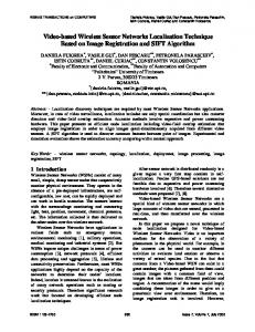
Figure 1: Various Iterative approaches in NLS and ML algorithms. 48
Signal & Image Processing : An International Journal (SIPIJ) Vol.6, No.1, February 2015
3.1. Nonlinear Least Squares (NLS) approach for TOA based positioning The nonlinear least squares method is simple and is an obvious choice when the noise information is not available. The NLS approach directly tries to minimize the least square cost function obtained from equation (4) and is as follows: Based on equation (4), the NLS cost function is represented as: (11)
The smallest value in the NLS cost function
is equal to the NLS position estimate
and is given by: (12) And obtaining xˆ is not easy, since both the local and global minimum values are contained in 2 dimensional surface of
.
In order to obtain the value of xˆ there are two ways, the first method is to use iterative local search algorithms based on an initial position estimate xˆ 0 , where 0 refers to the iteration number. If the value obtained after 0th iteration is approximately close to x, then xˆ can be iterated to the closest value of x. and second method is using the random search or the grid search techniques namely, the Genetic Algorithm (GA)[27] and Particle Swarm Optimization (PSO)[28][29]. In this paper, we limit our studies to the iterative search techniques. The three iterative approaches, namely, Newton Raphson iterative procedure, Gauss Newton iterative procedure, and Steepest Descent iterative procedure, are presented in the following subsections. 3.1.1. Newton Raphson Iterative procedure The iterative Newton – Raphson procedure for xˆ is given by:
(
) ( ( xˆ ) ) is the Hessian Matrix and ∇ ( J
(13) ) ( xˆ )) is the gradient vector
xˆ m +1 = xˆ m − H −1 J NLS ,TOA ( xˆ m ) ∇ J NLS ,TOA ( xˆ m )
(
Where H J NLS ,TOA
m
m
NLS ,TOA
measured at the m th iteration estimate. The algorithm for the Newton raphson procedure is summarized in Table 1. 3.1.2. Gauss Newton Iterative procedure The iterative Gauss - Newton procedure for xˆ is given by:
( (
xˆ m +1 = xˆ m + G T fTOA ( xˆ m )
))
−1
(
)(
G T fTOA ( xˆ m ) rTOA − fTOA ( xˆ m )
( ( ) ) is the jacobian matrix of f ( xˆ ) calculated at xˆ
Where G fTOA xˆ m
m
TOA
m
)
(14)
.
The algorithm for the Gauss- Newton iterative procedure is summarized in Table 2:
49
Signal & Image Processing : An International Journal (SIPIJ) Vol.6, No.1, February 2015 Table 1: Newton Raphson Iterative Procedure algorithm
Algorithm 1: Newton Raphson Method Input:
K = number of anchor nodes M = number of iterations X = {set containing all anchor nodes}; Initialize µ Output: estimated coordinates X (M) = [x1, y1] T Initialization: a random point x (0) For i=1: M do For j=1: K do
డమ ಿಽೄ,ೀಲ ሺ௫ሻ డమ ಿಽೄ,ೀಲ ሺ௫ሻ
H = డమ End
G=൦
డቀಿಽೄ,ೀಲሺ௫ሻቁ డ௬
డ௫డ௬
మ ಿಽೄ,ೀಲ ሺ௫ሻ డ ಿಽೄ,ೀಲ ሺ௫ሻ డ௫డ௬ డ௬ మ
డቀಿಽೄ,ೀಲሺ௫ሻቁ డ௫
డ௫ మ
൪
X = x − H −1G End Table 2: Gauss Newton Iterative Procedure algorithm
Algorithm 2: Gauss Newton method Input: K = number of anchor nodes M = number of iterations X = {set containing all anchor nodes}; Output: estimated coordinates X (M) = [x1, y1] T Initialization: a random point x (0) For i=1: M do For j=1: K do
ۍ డ௫ ێ ێడඥሺ௫ି௫మሻమାሺ௬ି௬మሻమ G=ێ డ௫ . ێ . ێ ێడඥሺ௫ି௫ಽሻమାሺ௬ି௬ಽ ሻమ ۏ డ௫ End డඥሺ௫ି௫భ ሻమ ାሺ௬ି௬భ ሻమ
−1
ې ۑ డඥሺ௫ି௫మ ሻమ ାሺ௬ି௬మ ሻమ ۑ ۑ డ௬ ۑ ۑ డඥሺ௫ି௫ಽሻమ ାሺ௬ି௬ಽሻమ ۑ ے డ௬ డඥሺ௫ି௫భ ሻమ ାሺ௬ି௬భ ሻమ డ௬
X = x + ( G T G ) GT ( r − f ( x) ) ;
End
3.1.3. Steepest Descent Iterative procedure The iterative procedure for the Steepest Descent iterative procedure is given by:
(
xˆ m+1 = xˆ m − µ∇ J NLS ,TOA ( xˆ m )
)
(15)
Where µ is a positive constant which commands the convergence rate and stability. 50
Signal & Image Processing : An International Journal (SIPIJ) Vol.6, No.1, February 2015
Table 3, summarizes the algorithm for Steepest Descent iterative procedure. Table 3: Steepest Descent Iterative Procedure algorithm
Algorithm 3: Steepest Descent method Input: K = number of anchor nodes M = number of iterations X = {set containing all anchor nodes}; Initialize µ Output: estimated coordinates X (m) = [x1, y1] T Initialization: a random point x (0) For i=1: M do For j=1: K do G=൦ End
డቀಿಽೄ,ೀಲ ሺ௫ሻቁ డ௫
డቀಿಽೄ,ೀಲ ሺ௫ሻቁ డ௬
൪
X = x − µG End
3.2. Maximum Likelihood approach for TOA based positioning The ML method maximises the probability density functions of the measured TOAs under the assumption that error distribution is known [30][31][32][33][34]. The maximization of the measured TOAs using ML method corresponds to the weighted version of the Non-linear least squares approach [35]. We consider the logarithmic version of the equation (6):
1 T 1 −1 ln ( P ( rTOA ) ) = ln − ln ( rTOA − d ) CTOA ( rTOA − d ) 1/ 2 L /2 ( 2π ) C 2 TOA
(16)
The first term in the RHS is independent of x, and maximising equation (16) is equal to minimising the second term, and hence the ML estimate can be obtained as:
(17) Or we can write (18) Where J ML.TOA ( x%) is the ML cost function, which is of the form:
51
Signal & Image Processing : An International Journal (SIPIJ) Vol.6, No.1, February 2015
(19) The ML estimator is generalized to NLS method because under the assumption of zero mean 2 Gaussian noise, σTOA , k is large which corresponds to a large noise in rTOA, k , a small weight of 2 1/ σTOA , k is employed in the squared term
, and vice versa. And also
−1 2 when CTOA is very near to the identity matrix or σTOA , k k = 1, 2,....., K are identical [35].
3.2.1. Newton Raphson Iterative procedure The iterative Newton – Raphson procedure for xˆ is given by:
(
) (
xˆ k +1 = xˆ k − H −1 J ML ,TOA ( xˆ k ) ∇ J ML ,TOA ( xˆ k )
(
( ) ) is the
Where H J NLS ,TOA xˆ m
(
)
(20)
( )) is the
Hessian Matrix and ∇ J NLS ,TOA xˆ m
gradient vector
measured at the m th iteration estimate. 3.2.2. Gauss Newton Iterative procedure The iterative Gauss - Newton procedure for xˆ is given by:
( (
)
(
−1 xˆ k +1 = xˆ k + G T fTOA ( xˆ k ) CTOA G fTOA ( xˆ k )
))
−1
(
)
(
−1 G T fTOA ( xˆ k ) CTOA rTOA − fTOA ( xˆ k )
( ( ) ) is the jacobian matrix of f ( xˆ ) calculated at xˆ
Where G fTOA xˆ m
m
TOA
m
)
(21)
.
3.2.3. Steepest Descent Iterative procedure The iterative procedure for the Steepest Descent iterative procedure is given by:
(
xˆ k +1 = xˆ k − µ∇ J ML,TOA ( xˆ k )
)
(22)
Where µ is a positive constant which commands the convergence rate and stability.
4. SIMULATION AND RESULTS Computer simulations have been carried out to evaluate the performance of the localization algorithms. In this paper, we consider a 2D geometry of K=4 receivers with known coordinates at (0, 0), (0, 10), (10, 10) and (10, 0), while the unknown source position is assumed to be (x, y) = (2, 3), such that the source is located inside the square bounded by four receivers. The Signal- to Noise - Ratio (SNR) = 30dB has been assumed. The results of the simulations are averaged over 50 iterations. And the step size parameter µ = 0.01 is assumed for the Steepest Descent method. All the simulations have been conducted using MATLAB [TM] Version 7.10.0.499 (R2010A)on Microsoft Windows XP, Professional Version 2002, Service pack 3, 32 bit operating system installed on Intel[R], Core [TM] 2 Duo CPU, E4500 @ 2.20GHz, 2.19GHz, 2.0GB of RAM. We have estimated the X and Y position using Nonlinear Least Squares (NLS) approach. There are three main parts in the simulation, i.e., generating the range measurements, position 52
Signal & Image Processing : An International Journal (SIPIJ) Vol.6, No.1, February 2015
estimation using NLS estimator which is realized by the Newton Raphson, Gauss Newton and Steepest Descent methods and displaying the results. Figure 2(a), 2(c), and 2(e) show the Xestimate using Newton Raphson, Gauss Newton and Steepest Descent methods whereas Figure. 2(b), 2(d), and 2(f) show the Y- estimate using Newton Raphson, Gauss Newton and Steepest Descent methods respectively. In the 2D geometry, the x-axis represents the number of iterations, i.e., 50 iterations at 30 dB, whereas the y-axis represents the position of the both X and Y estimate. The initial guess for estimating the position is assumed at (3, 2). All the schemes provide the same position estimate upon convergence. It can be seen that the Newton Raphson and Gauss Newton methods converge in about 3 iterations while the steepest descent algorithm needs approximately 15 iterations to converge. We have estimated the X and Y position using Maximum Likelihood (ML) approach. And the structure of the simulation is same as in the first example where there are three main parts in the simulation i.e., generating the range measurements, position estimation using ML estimator which is realized by the Newton Raphson, Gauss Newton and Steepest Descent methods and displaying the results. Figure 3(a), 3(c), and 3(e) shows the X- estimate using Newton Raphson, Gauss Newton and Steepest Descent methods whereas Figure 3(b), 3(d), and 3(f) shows the Y- estimate in Newton Raphson, Gauss Newton and Steepest Descent methods respectively. In the 2D geometry the x-axis represents the number of iterations i.e., 50 iterations at 30 dB, whereas the yaxis represents the position of the both X and Y estimate. The initial guess for estimating the position is assumed at (3, 2). similar to the NLS approach, all the schemes provide the same position estimate upon convergence, it can be seen the Newton Raphson and Gauss Newton methods converge faster than the steepest Descent algorithm, Nevertheless, it is difficult to see that the Maximum Likelihood (ML) estimator is superior to the NLS approach in terms of positioning accuracy based on a single run. Table 4: Estimated TOA Position measurement for NLS method when the Number of Anchor Nodes, n=4
Method : NLS
Newton Raphson Approach Gauss Newton Approach Steepest Descent Approach
Time of Arrival Estimate X- Position Estimate in Y- Position Estimate in Meters Meters
1.97 2.09 2.07
2.96 3.04 2.99
Table 5: Estimated TOA Position measurement for ML method when the Number of Anchor Nodes, n=4
Method : ML
Newton Raphson Approach Gauss Newton Approach Steepest Descent Approach
Time of Arrival Estimate X- Position Estimate in Y- Position Estimate in Meters Meters
1.98 2.01 2.05
2.97 3.01 3.07
The result of the position measurement estimate of the both NLS and ML method is given in Table 4 and Table 5 respectively. From Table 4, it can be seen that all the approaches estimate the X and Y positions, and the results of the Gauss Newton approach is better when compared with the other approaches. From Table 5, it is clear that the Gauss Newton method is near to the true positions and is having higher localization accuracy and the other approaches have lower 53
Signal & Image Processing : An International Journal (SIPIJ) Vol.6, No.1, February 2015
localization accuracy. Comparing Table 4 and 5, the iterative Gauss Newton method of the Maximum Likelihood approach is the better approach having higher localization accuracy.
(a). Newton Raphson X estimate
(c). Gauss Newton X estimate
(e). Steepest Descent X estimate
(b). Newton Raphson Y estimate
(d). Gauss Newton Y estimate
(f). Steepest Descent Y estimate
Figure 2: Estimate of X and Y position Versus Number of Iterations in NLS Approach
54
Signal & Image Processing : An International Journal (SIPIJ) Vol.6, No.1, February 2015
(a). Newton Raphson X estimate
(c). Gauss Newton X estimate
(e). Steepest Descent X estimate
(b). Newton Raphson Y estimate
(d). Gauss Newton Y estimate
(f). Steepest Descent Y estimate
Figure 3: Estimate of X and Y position Versus Number of Iterations in ML Approach
55
Signal & Image Processing : An International Journal (SIPIJ) Vol.6, No.1, February 2015
(a). MSPE Newton Raphson approach
(b). MSPE Gauss Newton approach
(c). MSPE Steepest Descent approach Figure 4: Mean Square Position Error Comparison of Non-Linear Approaches
56
Signal & Image Processing : An International Journal (SIPIJ) Vol.6, No.1, February 2015
We estimate the Mean Square Position Error (MSPE) comparison of NLS and ML approaches with Cramer Rao Lower Bound for Time of Arrival based positioning, the range error variance 2 2 2 2 σTOA , k is proportional to d k with Signal to Noise Ratio (SNR) = d k / σTOA, k . The MSPE is defined as E
{( xˆ − x )
2
+ ( yˆ − y )
2
} . Here we compute the empirical MSPE based on 1000
independent runs, which is given as
∑
1000 i =1
( xˆ − x ) 2 + ( yˆ − y ) 2 /1000 where ( xˆi , yˆi ) , denotes
the position estimate of the i th run. The simulation is run for both the NLS and ML approaches for the iterative Newton Raphson, Gauss Newton and the Steepest Descent Techniques and the function for the CRLB is also included, and the results are depicted in Figure 4(a), 4(b) and 4(c) for the various approaches in both NLS and ML method. Both the axes employ dB scale in the range SNR ∈ [ −10, 40] dB. From the figures we say that the performance of the Gauss Newton based ML estimator is superior and achieves optimal estimation performance, while the other approaches are suboptimal. Hence the ML estimator is superior to the NLS approach and its MSPE can attain CRLB.
5. CONCLUSIONS The work presented addresses the problem of position estimation of a sensor node, using time of arrival measurements. The Cramer Rao Lower Bound for the position estimation problem has been presented and the two nonlinear approaches such as Nonlinear least squares and Maximum likelihood approaches have been presented. Further both the Nonlinear Least Squares and Maximum likelihood approaches use three iterative local search algorithms, namely, Newton Raphson, Gauss Newton and the steepest descent methods and the results of these techniques are compared. Extensive simulation reveals that the Maximum Likelihood approach is superior to Nonlinear least squares approach under line of sight measurements. And the Maximum likelihood approach based Gauss Newton method is having higher localization accuracy and its MSPE can attain CRLB at SNR = 20dB when compared to the other approaches.
REFERENCES [1]
[2]
[3] [4] [5] [6]
[7] [8]
[9]
Ravindra. S and Jagadeesha S N, (2013), “A Nonlinear Approach for Time of Arrival Localization in Wireless Sensor Networks”, 6th IETE National Conference on RF and Wireless IConRFW-13, Jawaharlal Nehru National College of Engineering, Shimoga, Karnataka, India 09-11-May, pp 35-40. Yerriswamy. T and Jagadeesha S. N, (2011), “Fault Tolerant Matrix Pencil method for Direction of Arrival Estimation”, Signal & Image Processing: An International Journal, Vol. 2, No. 3, pp. 42-46, 2011. The Federal Communications commission about “Emergency 911 wireless services”, http://www.fcc.gov/pshs/services/911-services/enhanced911/Welcome.html Stojmenovic I, (2005), Handbook of sensor networks algorithms and architectures. John Wiley and Sons. Karl H, Willing A, (2005), Protocols and architectures for wireless sensor networks. John Wiley and Sons. Patwari N, Ash J N, Kyperountas S, Hero III AO, Moses RL, Correal NS, (2005), “Locating the nodes: cooperative localization in wireless sensor networks”. IEEE Signal Process Magazine, 22:54– 69. Wang C, Xiao L. (2007), Sensor localization under limited measurement capabilities. IEEE Network, 21:16–23. Pawel Kulakowski, Javier Vales-Alonso, Esteban Egea-Lopez, Wieslaw Ludwin and Joan GarciaHaro, (2010), “ Angle of Arrival localization based on antenna arrays for wireless sensor networks”, article in press, Computers and Electrical Engineering Journal Elsevier, doi:10.1016/j.compeleceng.2010.03.007 H. Wymeersch, J. Lien and M. Z. Win, (2009), “Cooperative localization in wireless networks,” IEEE Signal Processing Mag., vol.97, no.2, pp.427-450. 57
Signal & Image Processing : An International Journal (SIPIJ) Vol.6, No.1, February 2015 [10] R Zekavat and R. M Buehrer (2011), “Handbook on Wireless Position estimation,” Hoboken, NJ: John Wiley & Sons, INC. [11] A. H. Sayed, A. Tarighat, and N. Khajehnouri, (2005), “ Network based wireless location: Challenges faced in developing techniques for accurate wireless location information,” IEEE Signal Processing. Mag., Vol. 22, no. 4, pp, 24-40. [12] Neal Patwari, Alfred O Hero III, Matt Perkins, Neiyer S Correal and Robert J O’dea. (2003), “Relative location estimation in Wireless sensor networks”. IEEE Transactions on Signal Processing, 51(8):2137-2148. [13] Yerriswamy. T and Jagadeesha S. N, (2012), “IFKSA- ESPRIT – Estimating the Direction of Arrival under the Element Failures in a Uniform Linear Antenna Array”, ACEEE International Journal on Signal & Image Processing, Vol. 3, No. 1, pp. 42 – 46, 2012. [14] Gezici S, Tian Z, Giannakis GB, Kobayashi H, Molisch AF, Poor HV, et al. (2005), “Localization via ultra-wideband radios,” IEEE Signal Process Mag.; 22:70–84. [15] A. Jagoe (2003), Mobile Location Service: The Definitive Guide, Upper Saddle River: Prentice- Hall. [16] M. Ilyas and I. Mahgoub, (2005), Handbook of Sensor Networks: Algorithms and Architectures, New York: Wiley. [17] J. C. Liberti and T.S. Rappaport, (1990), Smart Antennas for Wireless Communications: IS-95 and Third Generation CDMA Applications, Upper Saddle River: Prentice- Hall. [18] Yerriswamy. T and S. N. Jagadeesha, (2012) “Joint Azimuth and Elevation angle estimation using Incomplete data generated by Faulty Antenna Array”, Signal & Image Processing: An International Journal, Vol. 3, No. 6, pp. 99-114, December 2012. [19] Theodore S Rappaport et al (1996), Wireless Communication: principles and practice, Vol. 2, Prentice Hall PTR New Jersy. [20] S. M. Kay, (1988), Modern Spectral estimation: Theory and Application. Englewood Cliffs, NJ: Prentice Hall. [21] S. M. Kay, (1993), Fundamentals of Statistical Signal Processing: Estimation Theory, Prentice- Hall. [22] Ravindra. S and Jagadeesha S N, “Time of Arrival Based Localization in Wireless Sensor Networks: A Linear Approach”, Signal and Image Processing: An International Journal (SIPIJ), Volume 4, Number 4, pp 13-30, August 2013. DOI: 10.5121/sipij.2013.4402 [23] Y. Huang and J. Benesty, Eds., (2004), Audio Signal Processing for Next Generation Multimedia Communication systems, Kluwer Academic Publishers. [24] E. G. Larsson, ( 2004), “Cramer-Roa Bound analysis of distributed positioning in sensor networks,” IEEE Signal processing Lett., Vol. 11, no. 3, pp. 334-337, mar, 2004. [25] Feng Yin, Carsten Fritsche, Fredrik Gustafsson and Abdelhak M Zoubir, (2013) “ TOA- Based Robust Wireless Geolocation and Cramer Rao Lower Bound Analysis in Harsh LOS/NLOS Environments, IEEE Transactions on Signal Processing, (61),9,2243-2255. http://dx.doi.org/10.1109/TSP.2013.2251341 [26] D. J. Torrieri, (1984) “Statistical theory of passive location systems,” IEEE Transactions on Aerospace and Electronic Systems, vol 20, no.2, pp. 183-198. [27] K. W. Cheung, H.C. So, W.-K. Ma and Y.T.Chan, (2004) “Least squares algorithms for time-ofarrival based mobile location,” IEEE Transactions on Signal Processing, vol.52, no.4, pp.1121-1128. [28] C. Mensing and S. Plass (2006), “Positioning algorithms for cellular networks using TDOA,” Proc. IEEE International Conference on Acoustics, Speech and Signal Processing, vol. 4, pp. 513-516, Toulouse, France. [29] H. C. So and K W Chan, (2005) “A generalized subspace approach for mobile positioning with timeof-arrival measurements,” IEEE transactions on Signal Processing, Vol.53, no.2,pp 460-470. [30] H.-W. Wei, Q. Wan, Z.-X. Chen and S. -F. Ye, (2008) “Multidimensional Scaling – based passive emitter localization from range-difference measurements,” IET Signal Processing, vol.2, no.4, pp.415-423. [31] F.K.W. Chan, H.C.So, J. Zheng and K.W.K. Lui, (2008), “Best Linear Unbiased Estimator approach for time-of –arrival based localization,” IET Signal Processing, vol.2, no.2,pp.156-162. [32] J. C. Chen, R.E. Hudson and K. Yao, (2002), “Maximum-likelihood source localization and unknown sensor location estimation for wideband signals in the near field,” IEEE Transactions on Signal Processing, vol.50, no.8, pp.1843-1854. [33] G. C. Carter, Ed.(1993), Coherence and Time Delay Estimation: An Applied Tutorial for Research, Development, test, and Evaluation Engineers. New York: IEEE.
58
Signal & Image Processing : An International Journal (SIPIJ) Vol.6, No.1, February 2015 [34] M. Marks and E. Niewiadomska - Szynkiewicz, (2007), “Two-Phase Stochastic optimization to sensor network localization,” Proc. IEEE International Conference on Sensor Technologies and Applications, Valencia, Spain, pp. 134-139. [35] Y. T. Chan and K.C. Ho, (1994) “A Simple and Efficient estimator for hyperbolic location,” IEEE Transactions on Signal Processing, vol. 42, no. 8, pp. 1905 – 1915. [36] H. C. So, Y. T. Chan and F.K.W. Chan, (2008), “Closed-form formulae for optimum time difference of arrival based localization,” IEEE Transactions on Signal Processing, vol.56, no.6, pp. 2614-2620.
AUTHORS Ravindra. S. received his B.E., in Electrical and Electronics Engineering., and M.Tech., in Networking and Internet Engineering, from Visvesvaraya Technological University, Belgaum, Karnataka, India in 2006 and 2008 respectively. He is currently working towards a Doctoral Degree from Visvesvaraya Technological University, Belgaum, Karnataka, India. At present he is working as Assistant Professor, in Computer Science and Engineering department of Jawaharlal Nehru National College of Engineering (affiliated to Visvesvaraya Technological University), Shimoga, Karnataka, India. Dr. S.N. Jagadeesha received his B.E., in Electronics and Communication Engineering, from University B. D. T College of Engineering., Davangere affiliated to Mysore University, Karnataka, India in 1979, M.E. from Indian Institute of Science (IISC), Bangalore, India specializing in Electrical Communication Engineering., in 1987 and Ph.D. in Electronics and Computer Engineering., from University of Roorkee, Roorkee, India in 1996. He is an IEEE member. His research interest includes Array Signal Processing, Wireless Sensor Networks and Mobile Communications. He has published and presented many papers on Adaptive Array Signal Processing and Direction-of-Arrival estimation. Currently he is professor in the department of Computer Science and Engineering, Jawaharlal Nehru National College of Engg. (Affiliated to Visvesvaraya Technological University), Shimoga, Karnataka, India.
59