Department of Computer Science. Shanghai Jiao Tong University. 1954 Hua
Shan Road, Shanghai 200030, China. Abstract. The paper proposes reaction ...
Reaction Graph* Yuxi Fu Department of Computer Science Shanghai Jiao Tong University 1954 Hua Shan Road, Shanghai 200030, China
Abstract
As mathematical objects, they are not as simple as they could be. Linear logic ([11, 33]) was introduced as a modi cation of classical logic. One of its aims is to achieve a proof theory for classical logic comparable to that for constructive logic. Computational interpretation of the linear logic was initiated by Abramsky ([2]). He subsequently gave a process interpretation of linear proofs (confer [3]). The approach was further investigated by Bellin and Scott ([6]) using �-calculus. The underlying idea of the proof-as-process paradigm is that cut eliminations can be interpreted as communications. What is not so clear in the process interpretation is that it is the underlying graphs of derivations of proofs that are being coded up. In this paper we present reaction graphs as alternatives to interaction diagrams. Reaction graphs have inspiration from interaction diagrams. But the two di�ers signi cantly. Firstly there are two classes of nodes. The local nodes are unlabeled whereas the global nodes are labeled. Secondly there is only one kind of arrows. There is no structural di�erence between input and output arrows. In other words, computations are regarded as a symmetric operation. Thirdly the universal computing power is achieved by a simple form of duplication. The main motivation of reaction graphs however comes from the idea of proof-as-process discipline. The rewriting of the graphs, which models computations, attempts to capture the essence of communications in concurrency theory and cut eliminations in logic. Compared to the interaction diagrams, the selling point of reaction graphs is its simplicity. There are variants of reaction graphs that have more convenient expressive power. The design decision we have made for reaction graphs trades o� expressiveness for simplicity. The reaction graphs nevertheless are strong enough to capture most familiar aspects of computations. What is carried out in this paper can be seen in a di�erent angle as repercussion of Abramsky's proposal. We attempt to substantiate a process-as-proof paradigm, which should contribute to a better understanding of both
The paper proposes reaction graphs as graphical representations of computational objects. A reaction graph is a directed graph with all its arrows and some of its nodes labeled. Computations are modeled by graph rewriting of a simple nature. The basic rewriting rules embody the essence of both the communications among processes and cuteliminations in proofs. Calculi of graphs are identi ed to give a formal and algebraic account of reaction graphs in the spirit of process algebra. With the help of the calculi, it is demonstrated that reaction graphs capture many interesting aspects of computations.
1 Introduction Interaction diagrams are introduced in [24] as a diagrammatic description of mobile processes. There are three kinds of nodes. Free nodes are labeled; they represent free names in �-calculus. Parameter nodes are unlabeled; they correspond to local names. Input nodes are also unlabeled; they denote the input names. Arrows in interaction diagrams are classi ed into two groups. Input arrows model the input pre xes of �-processes whereas output arrows the output pre xes. An input arrow must point to an input node. When an output arrow ends with the node an input arrow starts, a communication can happen. Such a communication coalesces the start node of the output arrow and the end node of the input arrow, dragging the remaining arrows along the way. The communication also deletes the input and the output arrows. An interaction diagram is partitioned into regions, each of which representing a process. To achieve Turing computability, either recursion or duplication must be incorporated in the diagrammatic setting. Interaction diagrams are graphic representations of concurrent processes with changing access capability. *
Journal of Computer Science and Technology ,
13(6):510-530, 1998.
1
is a graph. Graphs will often be presented diagrammatically.
disciplines. Apart from the interaction diagram, other forms of diagrammatic representation of computing objects have also been proposed. Milner for example has studied �-nets ([19]) and Lafont has introduced interaction nets ([14]) and interaction combinators ([15]). Section 2 de nes in an informal way reaction graphs and reactions. Section 3 identi es two calculi of graphs in the spirit of process algebra. The terms of the calculus are the formal counterparts of the reaction graphs described in the previous section. Section 4 explains how reaction graphs capture some interesting aspects of computations. Some remarks are made in the nal section. The material in this paper has been announced in [9].
2.1 Simple Reaction Graph
Reaction graphs have two kinds of nodes. There are local nodes and global nodes. A local node is unlabeled, represented in a graph by a circle. A global node is labeled with a small case letter, denoted by a circle with the label written inside the circle. j mj local global A simple reaction graph is a nite directed graph with each of its arrows labeled by either + or ;. In addition, for each name m there is at most one node labeled by m. Loops are allowed, meaning that an arrow can start and end with a same node. There can be more than one arrow from one node to another. The following is an example of simple Reaction graphs try to represent the topological reaction graph. structures of the communicabilities of processes and jH ; the underlying graphs of proof derivations in a disHHHj j tilled form. Computations of reaction graphs model (1) + + *� + �� communications and cut eliminations. Technically ?? � � � reaction graphs are directed graphs with each of mj� ��; their arrows labeled by either + or ;. The labels indicate polarities of arrows and decide what can In sequel, we will omit the label `+' and shorten the react upon each other. A reaction graph may have label `;' to `-'. The above graph will look like some of its nodes labeled. These nodes are important in that they are the channels through which jH environments interact with the graph. Normally we HHHj j are not interested in those reaction graphs which do (1) ��*� ?? � not have any labeled nodes. In sequel, the labels of � � mj� �� nodes will be drawn from a set N of names ranged over by lower case letters. Throughout this paper, we assign a number to each of the reaction graphs Next is another example of simple reaction graphs. given in the paper. We will refer to a reaction graph aj bj by Gi where i is the number assigned to it. ;�; 6 The graphs we are interested in this paper are - 6; ; nite directed graphs with possibly more than one (2) ?; � j arrow from one node to another. The start node mj; and the end node of an arrow can be the same. The following is a formal de nition of such graphs. A formal de nition of simple reaction graph goes De nition 2.1 A nite directed graph is a quadru- as follows: ple hN; E; d0; d1i where both N and E are nite sets, De nition 2.2 A simple reaction graph is a sexd0 and d1 are functions from E to N that specify tuple hN; E; d0; d1; o; ei such that hN; E; d0; d1i is a respectively the start and the end nodes of arrows. nite directed graph, o is a partial function from N to N that is injective on the domain of de nition, Graphs may be given by diagrams. For instance and e is a function from E to f;; +g. jH The set f;; +g will be ranged over by p. De ne ;p HHH j j to be +(;) when p is ;(+). *� � � ?? � Let F; G; � � � range over reaction graphs. There j� ��� � are four operations on reaction graphs that can be introduced at this stage. The composition of two
2 Reaction Graph
2
2.2 Atomic Reaction
graphs F and G, notation F jG, is obtained from the union of F and G by identifying global nodes with same labels. The composition G1 jG2, of the simple reaction graphs in (1) and (2), is the following simple reaction graph:
Simple reaction graphs are meant to be computing agents. The nodes of a graph are like atoms. They react with one another, producing new atoms. The arrows indicate the valences the nodes can exhibit. For example, in the simple reaction graph G7 given j j j a b in section 2.1, the node labeled m shows up negative I@ - 6 ;; @ �; 6 valence to the node labeled n. (3) - 6@-@ ; ? @ ; An atomic reaction happen between two local R @ ; j - mj� j nodes or between a local node and a global node. When two local nodes show up opposite valences For each label m, ( )nm is a unary operation on to a same node, they can react by removing the reaction graphs. Gnm is obtained from G by re- two arrows indicating the valences and coalescing moving the label m from the graph. For instance, the two nodes. This computation step can be illusG1nm is the following graph: trated by the following simple reaction rule, where p 2 f;; +g: jH p ej�-p j ) j j HHH je (A1) j j (4) * � � ?? �� Here the node with the incoming arrows labeled p j� ���� and ;p acts as a catalyst. A circle with another circle inside denotes either a global node or a local The third operation is substitution. For names a node. The rule implies that a catalyst can be either and b, G[a=b] is the graph obtained from G by local or global. Reactions in our formalism reminds relabeling the node labeled b by a. For instance, one of the chemical reactions in the abstract chemG1[n=m] is the following graph: ical machine ([5]). If a local node and a global node show up opposite valences to a catalyst, they can jH also react by removing the two arrows indicating the HHH j valences and coalescing the two nodes. But now laj (5) *� � � ?? bel the resulting node by the same name as the label � nj� ���� of the global reacting node. This computation step can be illustrated by the following atomic reaction Notice that distinct global nodes of G might col- rule: p ej�-p mj ) mj j lapse into one as a result of substitution operation. (A2) je The fourth operationp is also unary. For each pair of names m; n, G[m!n], where p 2 f;; +g, is what Another situation arises when two global nodes with is obtained by adding to G an arrow with label p opposite valences or neutral valences are connected starting from the node labeled by m and ending at to a same node, as shown in the following graph: ; b] is the the node labeled by n. For example, G2 [a! p ej�-p mj nj(8) following graph: If we merge the two nodes labeled respectively by n aj - - bj and m, we wouldn't know how to label the resulting � ; ;6 (6) - 6; node. We therefore disallow reactions between two ; ?j;; global nodes. � j m Applying the atomic computation rules, we can rewrite simple reaction graphs. Graph G1 can be In case there isn't a node labeled by m (n) in G, the rewritten in three ways. The global name labeled operation has to add to the graph a node with that by m can act as a catalyst for two reactions, which ; n] label. This operation is a derived one. G[m! are computationally the same: can be de ned as the composition of G with the jH j�� following simple reaction graph: �H H Hj j ) 6 (7) mj - - nj * � � ?? ?j ��- � � j � m m � � The four operations de ned here also apply to reaction graphs that are not simple. 3
In graph G1, the node on the right can also be a catalyst that triggers a reaction. The reduction can be pictured as follows:
jH -
HHH j * � � ??���- � mj� � �
j )
j ; ; j 6 @I@- j
-�� mj��� 6-
We say that the simple reaction graph
j
j
; 6 j; @I@- j
The above two reductions are independent; they can happen in parallel. In our interleaving scenario, a choice has to be made as to which reduction is conducted rst. Nondeterminism is therefore intrinsic. For two independent reductions, the choice of reduction order is immaterial. For instance, the above two computations can be continued, ending with a same graph:
j���-
6 ?j
�� ) mj? (
m
is the internal structure of the molecule and the three nodes the component nodes of the molecule. A component node of a reaction graph can itself be a molecule:
j ; ; j 6 @I@- j
-�� mj��� 6-
j
whose internal structure is the reaction graph
j ; ; j 6 @I@- j
The middle simple reaction graph is normal; it cannot be reduced further. Reactions are not always independent. Take the next reduction sequence for instance.
j
- 6 - ;;
j
j
I@ ) 6-@ j�- @ j
j which is not simple.
Reaction graphs and molecules are mutually de-�� ned as follows: ?j; � j j? � A simple reaction graph is a reaction graph; � If G is a reaction graph, then one can get anHere the second reduction depends causally on the other reaction graph by placing a square in G rst one. Causality is an important aspect of any that covers at least one non-global node. The model for computations. nodes lie inside a square must be either local or molecular � A molecular node, or molecule, is a reaction 2.3 Reaction Graph graph encompassed in a square. A reaction graph can be repetitively rewritten by In a sense, the internal structure of a molecule is applying (A1) and (A2). This procedure must ter- not completely shielded from outside. In a reaction minate in a nite number of steps as each step de- graph, an arrow pointing to a molecular node accreases the number of arrows by two. To achieve tually points to a component node of the molecule. the universal computing power, we must go beyond Similarly, an arrow comes from a molecule actually comes from a node inside the molecule. the simple framework. The solution we are interested in is to introduce When drawing a molecule, the following condianother kind of nodes, called molecular nodes. A tions should be observed: molecule consists of a set of non-global nodes with � all the arrows between the nodes inside a coupling relationships among them. Graphically a square lie inside the square as well; molecule is described by a square so that all the relevant nodes lie within the square. The following � all the arrows between the nodes outside a square lie outside the square as well; is a molecule:
6
)
4
� a node can not lie on the edge of a square; � squares can be nested but not overlapped.
As we have said, this reduction is carried out in two stages. First the molecule involved in the reaction makes a local copy of its internal structure, giving rise to G9:
The following is not a reaction graph:
j
mj
; 6 - j -�� j; I@- j @
j
6 ;; 6 ? � j j� - mj; -
(9)
-
It contains a global node. The diagrammatic rep- and then the local copy participates in the reaction. resentation violates our requirement in three ac- The following is another example of molecular recounts: Firstly the loop on the left node props out duction of the big square. Secondly the arrow points to the j j j right node does not come from a component node. ; ; ; ; j -- j 6 ) 6 j 6 Finally the two squares overlap.
I@@ j
2.4 Molecular Reaction
Molecular reactions allow a molecule to duplicate itself, thus permitting divergent computations. When a local node reacts to a molecule, it rst makes a copy of the internal structure of the molecule and then the local node reacts to the associated component node in the replica. The following molecular rule intend to capture the intuition:
jp- ej�-p + �� j ej�-p ��
(M1)
Similarly we have: mjp- ej�-p (M2)
+ �� ej�-p mj ��
j
- 6 ;; 6 ?; mj� j
)
j
6 I@@ j
j -- j
j�
6
)
j
j
- j�
j
6
j
The internal structure of the molecule was rst copied. The internal structure of the smaller molecule in the replica is copied afterwards. Then the reaction happened. In general a molecular reaction should make successively internal structures of nested molecules until the relevant atom becomes nude. The reaction then follows. For simplicity, we do not consider nested molecular reaction in this paper. We also disallow reactions between two molecular nodes. A molecular node can not act as a catalyst.
�� j �� �� j ��
2.5 Guarded Graphs
�� j �� j
j
I@@ j
The molecular reaction rule does not cover the situation where one of the reacting atom lie in a nested molecule. In the following reduction, a local node reacts to an atom inside a molecule inside another molecule:
�� j ��
Here is an example of molecular rewriting:
� j;;
A molecular node in a reaction graph can react to di�erent atomic nodes via di�erent arrows. In the following reaction graph both the node a and the
j
-
6 ; � - ; 6 ?j;� j m
aj
j - mj
? ?� j nj
6-
bj
node b can react to a node in a replica of the 5
molecule. In many situations it is convenient to the labels be drawn from the set Z of integers, we have guarded molecules. A guarded molecule is a get polyadic reaction graphs. The following is a molecule that has a principal component node that polyadic reaction graph: is local. In a graph, every guarded molecule has a jH -4 principal arrow that starts from the principal comHHHj j ponent node of the molecule and ends at an atomic 1 2 *� -3�� node outside the molecule. The molecule in the fol?? � � � lowing graph is guarded. mj� �� -1 -
aj
j - mj
If we go to extreme, we can draw the labels from a singleton set. This is the same as not to label arrows at all. Below is such a graph
6-
? ? nj� � j
bj
jH
HHHj ��*� ?? � � � j m� ��
The bottom node in the molecule is the principal node and the principal arrow is indicated by an enlarged dot at the junction of the arrow and the square. The only way an atomic node can react upon a guarded molecule is with the principal node through the principal arrow. For instance there is only one initial reaction in the above graph. By a guarded reaction graph we will refer to either a simple reaction graph or a reaction graph with guarded molecules. The molecular rules are
We call such graphs monadic reaction graphs1 . In a polyadic reaction graphs, an arrow labeled by i can react to an arrow labeled by ;i if they point to a same atom.
3 Calculi of Graphs
��
jp- ej�-p � j
Instead of giving a formal de nition of reaction graphs in a set theoretical setting, we de ne in this section calculi for reaction graphs in the spirit of process algebra ([16, 20, 18]). Two languages will be proposed. One is for the plain reaction graphs. The other is for the guarded reaction graphs. Strictly speaking, the terms of the calculi are more general than the graphs. But the generality is only technical. Graph terms are those terms that correspond precisely to reaction graphs. The non-graph terms can be coded up in graph terms. The encoding is faithful both operationally and algebraically. Similarly one can also identify a class of terms in the calculus of guarded reaction graphs that are in bijective correspondence to guarded graphs. Any term can be transferred to one such term. The transformation also preserves operational and algebraic semantics. We will concentrate on polyadic reaction graphs. All results in this section hold in the diadic and monadic cases as well.
��
(M1')
and
+ �� �� j ej�-p � j �� ��
��
mjp- ej�-p � j
��
(M2')
j
+ �� �� -p ej� � j mj �� ��
Guarded reaction graphs are introduced because they have better algebraic properties and are easier to implement.
3.1 Calculus of Graphs
The calculus of graphs intends to give term representations of reaction graphs. We rst de ne the set of terms by the following abstract syntax:
2.6 Classi cation of Graphs
The labels of the reaction graphs described so far P := 0 j mi [x] j (x)P j P jP 0 j !P; range over the set f;; +g. Only arrows with opposite labels can react upon each other. We will 1 Our convention on drawing diadic reaction graphs is now call such reaction graphs diadic. If instead we let causing confusion. Such ambiguity never arises in this paper. 6
where i 2 Z . Here m and x range over the set N of names. In (x)P , x is local, meaning that it can not be seen from outside. We will abbreviate (x1 ) : : :(xn )P to (~x)P . Terms of the from P jQ are composition terms. Terms of the form mi [x] are called atomic terms whereas those of the form !P molecular terms. In mi [n], m is subjective and n is objective. It is helpful to think of mi [n] as describing the situation where the datum n is stored at the i-th port of medium m. We say that an atomic term mi [n] is free in P if it is a subterm of P and both m and n are global in P . Let T be the set of all terms. We will adopt the so-called �-convention which says that replacing a local name in a term by a fresh name does not change the syntax of the term. For diadic graphs, the syntax of the calculus is de ned as follows: P := 0 j m[x] j m[x] j (x)P j P jP 0 j !P: And for monadic graphs, P := 0 j m[x] j (x)P j P jP 0 j !P: Before de ning the operational semantics of the calculus, we need to de ne a structural equivalence on the set of all terms. De nition 3.1 The structural relation = is the
where [] is the empty substitution. Substitutions will be ranged over by �. The operational semantics for the calculus of graphs is given in a reductional style rather than by a labeled transition system. It consists of the following reduction rules. Atomic Reduction
(x)(mi [x]jm;i[y]jP) ! (x)(P[y=x]) Molecular Reduction
mi [x]j!(y)(m;i[y]jP ) ! P[x=y]j!(y)(m;i[y]jP) Structural Rule
P ! P0 P jQ ! P 0jQ
P ! P0 (x)P ! (x)P 0
Let !+ (!� ) be the (re exive and) transitive closure of !.
Lemma 3.3 If P ! P 0 then P [y=x] ! P 0[y=x].
We now investigate the algebraic theory of the language. Suppose a is a global name in term P . least congruence on terms that contains: We say that a is an immediate barb of P, notation (i) P j0 = P , P1jP2 = P2jP1, and P1j(P2jP3) = P #a, if (P1 jP2)jP3; (ii) (x)0 = 0, (x)(y)P = (y)(x)P , (x)(P jQ) = � P = ai[x] for some i 2 Z ; P j(x)Q if x 62 gn(P ). We think of = as a grammatic equality. So P=Q � P = P1jP2 and either P1#a or P2#a; means that P and Q are the same term. 0 0 A term P is in standard form if it is either 0 or � P = (x)P and P #a and x 6= a. of the form, Write P #Q if 8a 2 N :P #a $ Q#a. We say that a is a barb of P, notation P +a, if Q exists such that (~x)(A1 j : : : jAij!M1j : : : j!Mj ); P !� Q#a. For two terms P and Q, write P +Q where i+j � 1, A1; : : :; Ai are atomic terms and if 8a 2 N :P +a , Q+a. A binary relation R is M1 ; : : :; Mj are in standard forms. In the latter case barbed if P RQ implies P +Q. Our de nition of barb A1 ; : : :; Ai will be called the atomic components of is non-standard in that we completely ignore the P and !M1; : : :; !Mj the molecular components of internal structure of molecules. It is reasonable for P. the version of barbed bisimilarity introduced below. Lemma 3.2 For any term P there is a term Q in Lemma 3.4 If P =Q then P #Q and P +Q. standard form such that P =Q. In sequel the notation [y=x] stands for an atomic Lemma 3.5 If P ! Q and Q+a then P +a. substitution. The result of substituting y for x throughout P is denoted by P [y=x]. Local names There are many ways to de ne an equivalence rein P need be renamed to avoid y being captured. lation on processes ([23, 16, 26, 27, 25]). What A substitution [y1 =x1 ] : : :[yn =xn] is a concatenation seems most suitable to the terms of the calcuof atomic substitutions. The e�ect of a substitution lus of graphs is the barbed bisimilarity introduced on a term is de ned as follows: in [21]. Barbed bisimulations are de ned in terms of a reduction semantics and an observation preddef P [] = P icate. The de nition below is closer to the version P[y1=x1] : : :[yn =xn] def = (: : :P [y1=x1] : : :)[yn =xn] of Honda and Yoshida ([13]). 7
Proof: Suppose P � Q and P[y=x] ! P 0. By theorem 3.9, (x)(P ja0[y]ja0[x]) � (x)(P ja0[y]ja0[x]) for a fresh name a. Assuming x 6= y, one has
De nition 3.6 Let R be a subset of T �T . The relation R is a barbed bisimulation if it is barbed and whenever P RQ then for any term R and any sequence ~x of names, it holds that (i) if (~x)(P jR) ! P 0, then there exists some Q0 such that (~x)(QjR) !� Q0 and P 0RQ0; (ii) if (~x)(QjR) ! Q0 , then there exists some P 0 such that (~x)(P jR) !� P 0 and P 0RQ0. The barbed bisimilarity � is the largest barbed bisim-
(x)(P ja0[y]ja0[x]) ! P [y=x] ! P 0
By de nition, (x)(Qja0[y]ja0[x]) !� Q0 such that P 0 � Q0 and P 0+Q0. So the communication between a0[x] and a0 [y] must have happened before reaching Q0. It can be easily seen from lemma 3.3 that the ulation. communication through a can happen in the very According to the de nition, one has that !!P � 0 rst place: and !mi [x] � 0. (x)(Qja0 [y]ja0[x]) ! Q[y=x] De nition 3.7 Let R be a subset of T �T . The !� Q0 : relation R is a barbed bisimulation up to � if it is barbed and whenever P RQ then for any term R and So P[y=x] ! P 0 is matched by Q[y=x] !� Q0 . 2 any sequence ~x of names, it holds that (i) if (~x)(P jR) !� P 0, then there exists some Q0 3.2 Calculus of Guarded Graphs such that (~x)(QjR) !� Q0 and P 0 � R � Q0 ; (ii) if (~x)(QjR) !� Q0 , then there exists some P 0 The reaction graphs are simpler than the guarded such that (~x)(P jR) !� P 0 and P 0 � R � Q0. reaction graphs. But the latter enjoys a better algeCare should be given to proofs using bisimulation braic theory, as will be shown below. The terms of the calculus of guarded reaction graphs are de ned up to technique ([29]). as follows:
Lemma 3.8 If R is a barbed bisimulation up to �, then R ��. Theorem 3.9 Suppose P � Q. Then (i) P jR � QjR for any R 2 T ; (ii) (x)P � (x)Q. Proof: (i) If P � Q then P jO � QjO. Consider R def = f(P jO; QjO)jP � Q ^ O 2 T g[ �. Suppose (~x)(P jOjR) ! P 0. Then by de nition some Q0 exists such that (~x)(QjOjR) !� Q0, P 0 � Q0 and P 0+Q0 . Hence R is a barbed bisimulation. (ii) If P � Q then (y)P � (y)Q. This can be proved by showing that R def = f((~y)P; (~y)Q)jP � Qg is a barbed bisimulation. Suppose (~x)((~y)P jR) ! P 0. Then (~x)(~y)(P jR) ! P 0. By de nition, (~x)(~y)(QjR) !� Q0 such that P 0 � Q0 and P 0+Q0 . Therefore R is a barbed bisimulation. 2 Unfortunately � is not a congruence relation. For
P := 0 j mi [x] j (x)P j P jP 0 j mi (x)�P; where i 2 Z . The operational semantics of this calculus is de ned similarly to the one for the calculus of graphs. Only the molecular rule need be rede ned. Molecular Reduction
mi [x]jm;i(y)�P ! P[x=y]jm;i(y)�P: The algebraic theory of this language can be studied in completely the same way as we have done with the calculus of graphs. All results in section 3.1 also hold for the calculus of unguarded graphs. However the bisimilarity for the terms of the calculus of guarded graphs enjoys much better algebraic properties as the following theorem shows.
Theorem 3.11 The barbed bisimilarity is a con-
a counter example, notice that
gruence equivalence.
(x)mi [x] � (x)(a)(ai [x]j(b)(b0[a]jb0[m])):
Proof: We only have to prove that if P � Q then mi (x)�P � mi (x)�Q. Let R be the following relation 8 9 P � Q = < ((~x)(Rjmi (x)�P); (~x)(Rjmi (x)�Q)) R 2 T ; : : ~ x2N
But !(x)(a)(ai [x]j(b)(b0[a]jb0[m])) is clearly not bisimilar to !(x)mi [x] as the former is barbed bisimilar to 0 whereas the latter is not. This is part of the reason to introduce guarded molecules. Before ending this section, we prove an important technical lemma.
Suppose (~x)(Rjmi (x)�P) ! P 0. There are two cases:
Lemma 3.10 If P � Q, then P [y=x] � Q[y=x]. 8
� (~x)(Rjmi (x)�P ) ! P 0 is caused by a commu-
where x1; : : :; xn are the global names in P, then g(!P) is the following reaction graph:
nication within R. P 0 must be of the form (x~0 )(R0j(mi (x)�P)�). Then obviously
i xj
(~x)(Rjmi (x)�Q) ! (x~0)(R0 j(mi (x)�Q)�): By lemma 3.10, (x~0 )(R0 j(mi (x)�P)�)R(x~0 )(R0 j(mi (x)�Q)�):
� '$ � � � &% @xj 1; n xj
� (~x)(Rjmi (x)�P ) ! P 0 is caused by a communication between R and mi (x)�P . Then P 0 is of the form (x~0)(R0 jP[y=x]jmi(x)�P ). Similarly This completes the de nition of g. Suppose P is a graph term. The following properties are obvious: (~x)(Rjmi(x)�Q) ! (x~0)(R0 jQ[y=x]jmi(x)�Q): (i) if P ! Q, then g(P) ! g(Q); (ii) if g(P) ! G, then Q exists such that P ! Q and g(Q) is G. Now
On the other hand, it is clear that every reaction graph can be translated into a graph term. The two translations are in an obvious sense reversible to each other. How about the non-graph terms? The fact of the matter is that the di�erence between graph terms 2 and non-graph terms is only technical. There is a translation from terms to graph terms that preserves both operational and algebraic semantics. 3.3 Graph Terms First we de ne an auxiliary translation ( ) , where A graph term P is a term such that none of is a nite set of names: its molecular subterms contains any free atomic components. Graph terms correspond to reaction (0) def = 0 graphs. def (P jQ) = (P ) j(Q) Lemma 3.12 If P ! Q and P is a graph term, ((x)P ) def = (x)(P ) [fxg then Q is a graph term. (!P ) def = !P An inductive de nition of a translation g from def graph terms to reaction graphs goes as follows: (mi [x]) = mi [x]; when fm; xg \ 6= ; � g(0) is the empty reaction graph; (mi [x]) def = (a)(ai [x]j(b)(b0[a]jb0[m])); when fm; xg \ = ;: � g(mi [x]) is the following reaction graph: Lemma 3.13 For a term P in the calculus of xj i - mj graphs and a nite set of names , (P) !� P and (P) � P . which is a basic building block in the construction of reaction graphs; The translation can then be de ned as follows: � g((x)P) is the reaction graph g(P)nx; 0� def = 0 def � � g(P jQ) is the reaction graph g(P)jg(Q); (mi [x]) = mi [x] (P jQ)� def = P � jQ� � if g(P) is the reaction graph ((x)P)� def = (x)P � i j x (!P)� def = !(P � ); :
(x~0 )(R0 jP[y=x]jmi(x)�P) � R � (x~0 )(R0 jQ[y=x]jmi(x)�Q) by theorem 3.9 and lemma 3.10. Conclude that R is a bisimulation up to �.
� '$ � � � &% @xjn 1; xj
It is clear that if P is a term then P � is a graph term. The following two theorems guarantee that we do not lose any expressive power by restricting our attention to graph terms. 9
Corollary 3.20 For terms P and Q in the calculus of guarded graphs, P � Q if and only if Pb � Qb .
Theorem 3.14 Suppose P and Q are terms in the calculus of graphs. Then (i) if P ! Q, then P � !+ Q� ; (ii) if P � ! P 0, then P1 exists such that P ! P1 , P 0 !+ P1� and P 0 � P1�. Proof: (i) If P ! Q is caused by an atomic communication, then clearly P � ! Q� . If P ! Q
Results in this section substantiate our claim that the calculus of (guarded) graphs is a formal language for (guarded) reaction graphs. If something can be coded up in the calculus, it can also be coded up in the reaction graphs and vice versa.
is caused by a molecular communication, then use lemma 3.13. (ii) Equally simple. 2 3.4 Equivalence of Calculi The terms of the guarded reaction graphs are betTheorem 3.15 P � P � for any term in the calcu- ter behaved. On the other hand the terms of lus of graphs. the unguarded reaction graphs have more concise representations. The two languages are Proof: The relation f(P; P �) j P a termg is a graphic however equivalent. The following translation from bisimulation up to �. 2 the guarded terms to the terms should look familiar: � � Corollary 3.16 P � Q if and only if P � Q . 0! def = 0 def ! Next we take a look at the graph terms in the cal(mi [x]) = mi [x] culus of guarded graphs. In the calculus of guarded (P jQ)! def = (P )! j(Q)! graphs, the graph terms are also strong enough to code up all the non-graph terms. The following sim((x)P)! def = (x)P ! ple translation is part of the encoding to be de ned (mi (x)�P)! def = !(x)(mi [x]j(P)! ): later. A reverse translation from the terms to the guarded 0 def = 0 def terms can be de ned as follows: mi [x] = (a)(ai [x]j(b)(b0[a]jb0[m])) 0? def = 0 P jQ def = P jQ def ? (mi [x]) = mi [x] (x)P def = (x)P (P jQ)? def = P ?jQ? m(x)�P def = m(x)�P: ((x)P )? def = (x)P ? Lemma 3.17 For a term P in the calculus of (!P )? def = m1i1 (x1 )�P1? j : : : jmji (xj )�Pj? ; guarded graphs, P !� P and P � P . Now the encoding: where m1i1 6=x1,... ,mji 6=xj for some j � 0 and j
j
0b def = 0 def d mi [x] = mi [x] Pd jQ def = PbjQb def d (x)P = (x)Pb
P = (x1)(m1i1 [x1]jP1) = � � � = (xj )(mji [xj ]jPj ): j
Here m1i1 [x1],. ..,mji [xj ] are all the atomic components of P whose subjects are not local in P and whose objects are local in P. Notice that when def j=0, m1i1 (x1 )�P1?j : : : jmji (xj )�Pj? is 0. d b mi (x)�P = mi (x)�P: Let's see an example: The proofs of the next three results are similar to (!(x)(y)(m0 [x]jn0[y]jn0[y]j!Q))? those for the corresponding results in the calculus = m0 (x)�(n0 [y]jn0[y]j(!Q)?) of graphs. jn0(y)�(m0 [x]jn0[y]j(!Q)?) Theorem 3.18 Suppose P and Q are terms of the jn0(y)�(m0 [x]jn0[y]j(!Q)?): calculus of guarded graphs. Then (i) if P ! Q then Pb !+ Qb; The proof of the next theorem is similar to that of (ii) if Pb ! P 0 then there exists some P1 such that theorem 3.14. P ! P1, P 0 ! Pc1 and P 0 � Pc1. Theorem 3.21 Suppose P and Q are terms of the Theorem 3.19 For a term P in the calculus of calculus of graphs. Then guarded graphs, P � Pb. (i) if P ! Q then P ? !+ Q? ; j
j
10
(ii) if P ? ! P 0 then P1 exists such that P ! P1 , P 0 ! (P1)? and P 0 � P1? . Suppose P and Q are terms of the calculus of guarded graphs. Then (i) if P ! Q then P ! !+ Q! ; (ii) if P ! ! P 0 then P1 exists such that P ! P1 , P 0 ! (P1)! and P 0 � P1! .
That is (~x)(Rj((!P)?)! ) ! (x~0)(R0 j((!(P�))?)! ):
� If (~x)(Rj!P) ! P 0 is caused by a communication between R and !P, then P 0 must be of the form (~x)(R0 jPi [a=yi ]j!P) for some a and 1 � k � j. Correspondingly k
k
The composition of the two translations is not an identity function in either way. But they are inverse to each other up to bisimilarity in the sense of the following theorem.
(~x)(Rj((!P)?)! ) ! (~x)(R0 j((Pi [a=yi ])? )! j((!P)?)! ): k
k
Theorem 3.22 The following properties hold: (i) if P is a term in the calculus of guarded graphs, then (P ! )? � P ; (ii) if P is a term in the calculus of graphs, then (P ? )! � P .
Clearly, ((Pi [a=yi ])?)! � ((Pi [a=yi ])? )! : k
k
k
k
By induction hypothesis, ((Pi [a=yi ])? )! � ((Pi [a=yi ])? )! � Pi [a=yi ]:
Proof: (i) The proof is carried out by induction on the structures of terms. The only non-trivial case is for molecular terms: ((mi (x)�P)! )? = (!(x)(mi [x]j(P)! ))? = mi (x)�((P)! )? : By lemma 3.17, P � P. By induction hypothesis, ((P)! )? � P and (P ! )? � P . Hence by theorem 3.11, ((mi (x)�P)! )? = mi (x)�((P)! )? � mi (x)�P � mi (x)�P � mi (x)�(P ! )? : This completes the proof of (i). (ii) Let R be the following relation: 8 9 P 2 T < = ?)! )) R 2 T ((~ x )(R j P ); (~ x )(R j (P : : ~ x names ; We show that R is a barbed bisimulation up to �. The only nontrivial case is when P is a molecular term. So assume (!P)? = m1i1 (x1 )�P1?j : : : jmji (xj )�Pj? :
k
k
k
k
k
k
So by theorem 3.9, (~x)(R0 j((Pi [a=yi ])?)! j((!P)?)! ) � (~x)(R0 jPi [a=yi ]j((!P)?)! ): k
k
k
k
It follows that (~x)(R0 jPi [a=yi ]j!P) � R � (~x)(R0 j((Pi [a=yi ])? )! j((!P)?)! ): k
k
k
k
So R is a bisimulation up to �. 2 For the sake of the next proof, let's annotate the barbed bisimilarity in the calculus of guarded graphs by a subscript g.
j
Theorem 3.23 (i) Suppose P and Q are terms in the calculus of guarded graphs. Then P �g Q if and only if P ! � Q! . (ii) Suppose P and Q are terms in the calculus of graphs. Then P � Q if and only if P ? �g Q? . Proof: (i) We rst show that if P �g Q then P ! � Q! . Consider the relation
Then ((!P)?)! is !(x)(m1i1 [x1]j(P1?)! )j : : : j!(x)(mji [xj ]j(Pj?)! ): Suppose R is a term and ~x is a sequence of names. Suppose further that (~x)(RjP) ! P 0. There are two cases: � If (~x)(Rj!P) ! P 0 is induced by a communication within R, then P 0 must be of the form (x~0 )(R0jP�). On the other hand, (~x)(Rj((!P)?)! ) ! (x~0 )(R0j((!P)?)! �):
S def = f(P ! ; Q! ) j P �g Qg: Suppose R is a term, ~x a sequence of names and (~x)(RjP !) ! P1. Then (~x)(R? j(P ! )? ) !+ P1? by theorem 3.21. By assumption and theorem 3.22, (P ! )? � (Q! )? . So (~x)(R? j(Q! )? ) !� Q2 for some Q2 such that P1? �g Q2. Hence by theorem 3.21,
j
(~x)((R? )! j((Q! )? )! ) !� Q!2 :
11
But
(~x)((R? )! j((Q! )? )! ) � (~x)(RjQ! )
De nition 3.24 Suppose C is a set of contexts in the calculus of graphs and R is a subset of T �T . The relation R is a barbed bisimulation with respect to C if it is barbed and whenever P RQ then for each C[] 2 C it holds that (i) if C[P] ! P 0, then there exists some Q0 such that C[Q] !� Q0 and P 0RQ0 ; (ii) if C[Q] ! Q0, then there exists some P 0 such that C[P] !� P 0 and P 0RQ0 . The barbed bisimilarity with respect to C , notation �C , is the largest barbed bisimulation with respect to C . When C includes all contexts, �C coincides with �.
according to theorem 3.22. So Q1 exists such that Q!2 � Q1 and (~x)(RjQ! ) !� Q1. It follows that S is a bisimulation up to �. (ii) Similarly we can show that if P � Q then P ? �g Q? . (iii) For guarded terms P and Q, if P ! � Q! , then by theorem 3.22 and (ii), P �g (P ! )? �g (Q! )? �g Q. (iv) The proof is similar to (iii). 2 The calculus of guarded graphs appears to have the edge over the calculus of graphs. But theorems 3.21, 3.22 and 3.23 establish the equivalence of the two languages. These results justify the decision to take reaction graphs as the basic computing agents.
In next section we show how the calculus of graphs act as a target language.
3.5 Graphs as Models
Suppose we have two calculi Li, i = 1; 2. Li is equipped with a reduction relation !i and an observational equivalence �i . The former de nes the operational semantics of Li while the latter characterizes its denotational semantics. A translation M from L1 to L2 should preserve at least the operational semantics of L1 , meaning that the following two complementary properties are satis ed:
� if S !1 T , then MS !2 MT; � if MS !2 T 0, then T exists such that S !1 T and T 0 !�2 MT The rst condition guarantees the soundness of the translation and the second ensures the faithfulness. As for the preservation of the observational equivalence, a natural requirement is (1)
S �1 T implies MS �2 MT:
If M is not meant to be part of a comparison of L1 against L2, but acts as a translation that interpret L1 in the target language L2 , then (1) is too strong a requirement. L2 might have far more discriminating power than L1. For example suppose L1 is a high level programming language and L2 is an assembly language. Normally we are not interested in the behaviour of two programmes MS and MT in the presence of an arbitrary piece of assembly code. All we care about is how they act in the presence of MP where P is a programme in L1. The next de nition to be introduced shortly come with these considerations. We rst introduce the notion of contexts in the calculus of graphs, which can be inductively de ned as follows:
4 Applying Reaction Graphs
In the end, a computational model has to be judged in practice. This section is devoted to demonstrations of the operational adequacy of reaction graphs. We rst explain how to regard a multiplicative linear logic proof as a reaction graph. The graph theoretical interpretation explicates that reactions in graphs are cut eliminations in an abstract setting. It is obvious that some reactions in a reaction graph can happen in parallel. The fact that sequential computations can be modeled in reaction graphs should indicate that graphs are concurrent computational agents. We will elaborate this point by giving a translation of the mini mobile processes to reaction graphs. By composing this translation with Milner's translation of the lazy �-calculus ([4, 1, 22]), we get immediately a translation of the latter in the calculus of graphs. A fallout of this fact is that reaction graphs possess Turing computability.
4.1 Proofs as Polyadic Graphs
Linear logic was proposed as a modi cation of classical logic ([11, 12, 33]). A computational treatment of the proofs of the classical linear logic is initiated in [2]. The idea is further explored in the setting of process algebras; see for example [6]. In this approach, a sequent proof is annotated with variables. A process interpreting the proof has free variables occurring in the conclusion of the proof as its free names through which it communicates with outside world. The Abramsky approach generalizes the proof-as-term paradigm to a proof-as-process paradigm. Cut eliminations are interpreted as process communications. Two things are noteworthy � [] is a context; with this interpretation. First in order to model � if C[] is a context, then C[]jP, (x)C[] are con- cut eliminations high up in a derivation tree, one needs reduction under pre xing. In [6], unguarded text. 12
pre xes are introduced to achieve that. Second the linear logic proofs are more symmetric than the �calculus can capture. The mismatch is due essentially to the functional nature of the communications in �-calculus. Another important point of the proof-as-process interpretation is that it tries to code up the underlying tree structures of the derivations of proofs. This is especially true for the multiplicative part of the linear logic. However in the process interpretation, the tree structures are buried in the syntax of the process calculus. In this section we take a look at Abramsky's translation of the multiplicative linear logic in our graph theoretical setting. We will see that the graph interpretation is more symmetric and re ects more faithfully the tree structures of proofs. There are four rules for the multiplicative linear logic, ignoring those rules for units: x : A; y : A? Axiom .. .. .F .G w~ : ;; x : A ~v : �; y : B
w~ : ;;~v : �; z : A B .. .F w~ : ;; x : A; y : B } w~ : ;; z : A}B .. .. .F .G w~ : ;; x : C ~v : �; y : C ? Cut w~ : ;;~v : � The basic idea of the interpretation is that a proof of the sequent x1 : A1 ; : : :; xn : An is interpreted by a reaction graph with n global nodes labeled respectively by x1 ; : : :; xn, as is shown below: xj '$ � i � � � j x&% xj 1 n
In the sequel, only relevant global nodes are displayed. The translation is inductively de ned as follows: � The axiom is interpreted by the following reaction graph:
0; xj;
j
@@ R0 yj
Formally the axiom is modeled in the calculus of graphs by the term (a)(x0[a]jy0[a]). Notice the symmetric roles of x and y in this term. 13
� If the premises of the -rule are interpreted respectively as the following reaction graphs:
'$'$ j xj y&% &%
then the conclusion of the rule is interpreted by the reaction graph:
'$'$ j j &% &% 1@@ R zj; ;0
Algebraically the interpretation is the term (x)(y)(z1 [x]jz0[y]jF jG). � If the premise of the }-rule is interpreted by the following reaction graph:
'$
j x&% yj then the conclusion of the rule is then interpreted by the reaction graph:
'$
j j &% -1@@ R zj; ;0 In the calculus of graphs, it is expressed as (x)(y)(z;1 [x]jz0[y]jF). � If the two premises of the cut rules are interpreted by the following reaction graphs:
'$'$ xj yj &%&%
then the conclusion of the rule is interpreted by the following reaction graph:
'$ '$ j &% &%
Theorem 4.2 Suppose P is a �-process. (i) if P ! Q then P y ! Qy; (ii) if P y ! P 0, then Q exists such that ! Q, P 0 !� Qy and P 0 � Qy.
More formally, the interpretation is the following term (z)(F[z=x]jG[z=y]). This completes the de nition of the interpretation. Cut eliminations for the multiplicative linear logic correspond to reductions in reaction graphs. A precise statement of this fact is omitted. Confer [6].
The algebraic properties of the �-calculus have been intensively studied ([30, 20, 31, 25, 26, 27, 32]). What is relevant to us in this paper is the barbed bisimilarity. Let's mention that a is an immediate barb of P, notation P #a, if � P � a(x):P or P � ax:P ; � P � P1jP2 and either P1#a or P2#a; � P � (x)P 0 and P 0#a and x 6= a. The barbed bisimulation (up to bisimilarity) can be de ned for the mini �-processes in completely the same way as for the terms of the calculus of graphs. The barbed bisimilarity is preserved by all but the input pre xing operator. Let C� be the set of all mini �-process contexts. The graph interpretations of the mini �-processes preserve the algebraic equality in the sense of the theorem below.
4.2 Processes as Diadic Graphs
Conceptually reactions that are not causally related can happen in parallel. Meanwhile reactions can be ordered in terms of enablement and the recursion mechanism. It is in this sense reaction graph rewriting captures concurrent computations. This section explains how to think of mobile processes as reaction graphs. The processes considered here are the so-called mini �-processes ([17]): P := 0 j m(x):P j mx:P j (x)P j P jP 0 j m(x)�P:
We will impose a syntactical equality on the set of all mini �-processes in the same way as we have done with the terms of the calculus of graphs. De nition 4.1 The structural relation = is the Theorem 4.3 Let � be the set fC[]y j C[] 2 C� g. least congruence on terms that contains: If P and Q are two mini �-processes and P � Q, (i) P j0 = P , P1jP2 = P2jP1, and P1j(P2jP3) = then P y �� Qy. (P1 jP2)jP3; (ii) (x)0 = 0, (x)(y)P = (y)(x)P , (x)(P jQ) = P j(x)Q if x 62 gn(P ). The operational semantics of the calculus is de ned The operational aspects of computations encapsuby the following two reduction rules: lated in reaction graphs are important enough to justify their introduction. This is reinforced by the m(x):P jmy:Q ! P [y=x]jQ simplicity of the structures of the reaction graphs. Reactions of graphs are cut elimination reincarm(x)�P jmy:Q ! m(x)�P jP[y=x]jQ nated in a graph theoretical setting. It is intended that reaction graphs abstract common geometric and the following three structural rules: structures from processes and proofs while reactions P ! P0 P ! P0 capture the dynamic recon gurations of the strucP jQ ! P 0jQ (x)P ! (x)P 0 tures typically found in concurrency theory and proof theory. More speci cally, a con guration of We now de ne a translation from the �-processes to the form reaction graphs. In view of the results in section 3, j j it su�ces to de ne a translation from the processes ;@@ to the calculus of guarded graphs: R j; ;+
5 Conclusion
0y def = 0
(m(x):P )y (mx:P)y (P jQ)y ((x)P)y (m(x)�P)y
def = def = def = def = def =
(a)(m[a]ja(x)?(a[a]jP y)) (a)(m[a]ja[x]ja(b)?Qy) P yjQy (x)P y m(x)�P y:
in a reaction graph is a cut. The recon guration of the cut by reaction eliminates the cut. On the other hand, a subgraph of the shape j mj ;@@ Rj ;+ e; 14
describes the situation in which m is ready to output through a channel which can also act as a channel for an input action. The reaction of the subgraph is a communication which instantiates the local name by m. We have emphasized that reaction graphs are computational objects on their own. It is however also worthwhile to see them as implementations of computational objects. Coming back to the view that reaction graphs are underlying structures of an abstract proofs, we can see that the calculus of graphs and the encodings of mini �-processes as graph terms are activities in a process-as-proof paradigm. The proof theoretical interpretation gives rise to a nonstandard understanding of mobile processes. Such an understanding demands a further stay-away from the familiar functional view of computations. Rewriting of reaction graphs reminds one of chemical reactions ([5]), which explains our choice of terminology. What comes natural in a chemical scenario is that things happen in parallel. We can also think of the calculus of graphs as a model for parallel computations. If two reactions do not result in con ict, they might as well proceed in parallel. To simplify the operational semantics for this parallel model, it is better to ban the rules (A2) and (M2). The simpli cation does not decrease the expressive power of the model though. From another viewpoint, elimination of (A2) and (M2) push the reaction graphs closer to proofs. The situation draw a resemblance to that where attention is paid to a sublanguage �I of the �-calculus ([28]). By adding the sequentiality combinator to the calculus of graphs, we get a process calculus, �calculus, that has been studied in [7, 8]. The syntax of the calculus also motivates a symmetric presentation of the �-calculus ([10]).
References
[5] G. Berry and G. Boudol. The Chemical Abstract Machine. Theoretical Computer Science , 96: 217{248, North Holland, 1992. [6] G. Bellin and P. Scott. On the �-Calculus and Linear Logic. Theoretical Computer Science, 135: 11{65, North-Holland, 1994. [7] Y. Fu. The �-Calculus. Proceedings of the In-
ternational Conference on Advances in Parallel and Distributed Computing, 74-81, 19-21
March, Shanghai, China, IEEE Computer Society Press, 1997. [8] Y. Fu. A Proof Theoretical Approach to Communications. ICALP'97, 7-11 July, Bologna, Italy, Lecture Notes in Computer Science 1256, Springer Verlag, 1997. [9] Y. Fu. Reaction Graphs. International Work-
shop on Formal Model of Programming and Its Applications, Beijing, 17-20 September, 1997. [10] Y. Fu. Symmetric �-Calculus. Journal of Computer Science and Technology , 13: 202{208,
[11] [12]
[13] [14] [15]
[1] S. Abramsky. The Lazy Lambda Calculus. Declarative Programming , ed. D. Turner, 65{ [16] 116, Addison-Wesley, 1988. [2] S. Abramsky. Computational Interpretations [17] of Linear Logic. Theoretical Computer Science , 111: 3{57, North Holland, 1993. [18] [3] S. Abramsky. Proofs as Processes. Theoretical Computer Science , 135: 5{9, North-Holland, 1994. [19] [4] H. Barendregt. The Lambda Calculus: Its Syntax and Semantics . Studies in Logic and Foundations of Mathematics, North-Holland, 1984. 15
1998. J. Girard. Linear Logic. Journal of Theoretical Computer Science , 50: 1{102, North-Holland, 1987. J. Girard. Towards a Geometry of Interaction. Categories in Computer Science and Logic , ed. J.W. Gray and A. Scedrov, Contemporary Mathematics, 92, 69{108, AMS, 1989. Honda and Yoshida. On Reduction Based Process Semantics. Theoretical Computer Science , 152(2):437{486, North-Holland, 1995. Y. Lafont. Interaction Nets. POPL'90 , 95{108, ACM, 1990. Y. Lafont. Interaction Combinators. Information and Computation , 137: 69{101. R. Milner. Communication and Concurrency , Prentice Hall, 1989. R. Milner. Functions as Processes. Journal of Mathematical Structures in Computer Science
2: 167{180, 1992.
R. Milner. The Polyadic �-Calculus: a Tutorial. Technical Report, Department of Computer Science , University of Edinburgh, 1992. R. Milner. �-Nets: a Graphical Form of �Calculus. ESOP'94, Lecture Notes in Computer Science 788, 26{42, Springer Verlag, 1994.
[20] R. Milner, J. Parrow and D. Walker. A Calculus of Mobile Processes. Information and Computation , 100: 1{40 (Part I), 41{77 (Part II), Academic Press, 1992. [21] R. Milner and D. Sangiorgi. Barbed Bisimulation, ICALP'92 , Lecture Notes in Computer Science 685{695, Springer Verlag, 1992. [22] L. Ong. The Lazy Lambda Calculus: An Investigation into the Foundations of Functional Programming . PhD thesis, Imperial College of
[23] [24] [25] [26]
[27] [28]
[29]
[30] [31]
[32] [33]
Science and Technology, University of London, 1988. D. Park. Concurrency and Automata on In nite Sequences. Lecture Notes in Computer Science 154, 561{572, Springer Verlag, 1981. J. Parrow. Interaction Diagrams. A Decade of Concurrency , Lecture Notes in Computer Science 803, Springer Verlag, 1993. J. Parrow and D. Sangiorgi. Algebraic Theories for Name-Passing Calculi. Information and Computation , 120, Academic Press, 1995. D. Sangiorgi. Expressing Mobility in Pro-
cess Algebras: First-Order and Higher-Order Paradigms . PhD thesis, Department of Com-
puter Science, University of Edinburgh, 1993. D. Sangiorgi. A Theory of Bisimulation for �-Calculus. CONCUR'93 , Lecture Notes in Computer Science 715, Springer Verlag, 1993. D. Sangiorgi. �I: A Symmetric Calculus Based on Internal Mobility, ICALP'95 , Lecture Notes in Computer Science, Springer Verlag, 1995. D. Sangiorgi and R. Milner. Techniques of \Weak Bisimulation Up To". CONCUR'92 , Lecture Notes in Computer Science, Springer Verlag, 1992. B. Thomsen. A Calculus of Higher Order Communicating Systems. POPL'89 , 143{154, Austin, Texas, USA, 1989. B. Thomsen. Plain CHOCS|A Second Generation Calculus for Higher Order Processes. Acta Informatica , 30: 1{59, Springer Verlag, 1993. B. Thomsen. A Theory of Higher Order Communicating Systems. Information and Computation , 116: 38{57, Academic Press, 1995. A. Troelstra. Lectures on Linear Logic. CSLI Lecture Notes, 1992. 16