REAL-TIME PATTERN ISOLATION AND RECOGNITION OVER IMMERSIVE SENSOR DATA STREAMS* CYRUS SHAHABI AND DONGHUI YAN Integrated Media Systems Center University of Southern California, Los Angeles, CA 90089
[email protected] Data streams appear in many recent applications, where data are constantly changing or take the form of continuously arriving streams. We focus on data streams generated by sensors for monitoring users in immersive environments. To recognize users' interactions, we need to analyze the aggregation of several sensor data streams and match the result to a set of known actions. In addition, we need to separate a continuous series of actions into recognizable atomic actions. Hence, we first propose a distance metric, weighted-sum Singular Value Decomposition (SVD), suitable for similarity measurement of immersive data sequences. Subsequently, we propose a mutual information based heuristic for separation of the action sequences. Finally, we perform several empirical experiments using real-world virtual-reality devices to verify the effectiveness of our approach.
1
Introduction
In traditional data management, dataset are usually stored in permanent storages such as disks or tapes and thus are persistent, most existing data management techniques are built on the assumption of persistent dataset. To answer a query on persistent dataset, we operate on the entire set of data and usually an exact answer to the query can be returned. In many recent applications, however, data usually take a different form, which are either constantly changing or continuously arriving; we call this type of data a continuous data stream (CDS). Examples of CDS include: stock price quotes, network traffic data, sensor data, and web access logs. Data generated as CDS are usually large in volume (e.g., network traffic data, sensor data) or constantly changing (e.g., stock price quotes), it is often impractical or unnecessary to answer queries based on the entire dataset. The challenges for query over CDS include the following: •
Queries must be answered based on limited amount of information rather than the entire dataset. This is due to the limit on the storage size of a database *This research has been funded in part by NSF grants EE-9529152 (IMSC ERC) and IIS0082826, NIH-NLM grant nr. R01-LM07061, DARPA and USAF under agreement nr. F3060299-1-0524, and unrestricted cash gifts from Okawa Foundation, Microsoft, and NCR.
• •
engine, usually only summary information can be stored. To determine what kind of summary information to store so that future queries can be answered correctly or approximately is a challenge. Queries usually need to be answered in real time. For some applications, such as manufacture controlling process using sensors, timely answer to a query is crucial. In some cases, data streams may come from different sources, where the answer to a query usually needs to aggregate information from some or all of these sources. This can be very difficult, to illustrate, consider the query “List the top ten web sites with most hits” using web logs from distributed web sources.
In this paper, we study problems arising from immersive environments, where a user is immersed into a virtual environment to interact with information and/or other users. In order to facilitate natural interactions (beyond keyboard and mouse), users in typical immersive environments are traced and monitored through various sensory devices such as: tracking devices on their heads, hands, and feet, video cameras and haptic devices. In earlier publications [21,23], we coined the term “immersidata” for data acquired from a user's interactions with an immersive environment. Immersidata type is: 1) multidimensional, 2) spatio-temporal, 3) continuous data stream (CDS), 4) large in size and bandwidth requirements, and 5) noisy. Here, we emphasize the CDS and multidimensional aspects of immersidata and consider immersidata as several continuous streams each generated by a sensor in an immersive environment. The goal is to understand a user's behavior by implicitly monitoring her interaction with the system. Realizing this goal can serve several purposes such as conducting human factor studies, improving system performance, customizing the environment towards the user's preferences, and identifying flaws and pitfalls in the environment. As a specific example of immersive environment and user behavior study through immersidata, throughout this paper we focus on recognizing hand motions by analyzing CDS generated from a virtual reality glove. We use datasets collected when performing American Sign Language (ASL) signs as well-defined hand motions. More details on our target application are provided in Section 2. In addition to the challenges mentioned earlier for the general CDS problem, our specific problem has at least two extra challenges: 1.
We are concerned about a sequence of data. A meaningful hand motion is formed by a sequence of data samples, rather than individual samples occurring in a data stream. In addition, a sequence for one hand motion has no fixed length, as different persons may finish a hand motion with different time duration while the data rate of the sensors are fixed (100 Hz). Hence, one needs to isolate a series of variable length motions into individual and recognizable actions.
2.
Our data are intrinsically high dimensional. Data from each individual sensor do not make much sense for us, rather data from all sensors together form a meaningful point in the hand motion trajectory. This is harder than the case for general CDS with data coming from distributed sources, where a loose aggregation is needed for the computation. In our case a much tighter aggregation is required, which essentially renders our problem to be a high dimensional one.
In order to recognize a series of patterns (with each being a sequence of data) over the aggregation of several sensor data streams, one needs to address two problems with interdependent solutions (chicken-and-egg problem). To illustrate, suppose as the result of an immersive interaction a series of p1 , p2 ,..., p N patterns have been generated. One problem is to isolate each pattern within the series, i.e., to identify when (say)
p1 ends and p 2 starts. The other problem is to actually
p1 as a known pattern. The interdependency is that in order to isolate p1 , it should be recognized as a known pattern. However, p1 must first be isolated
recognize
in order to be compared with a known set of patterns (termed vocabulary) to be recognized! We approach the problem in two steps. First we focus on isolated patterns and propose a similarity measure, weighted-sum SVD, to compare an input pattern to the members of a known vocabulary. Here, our weighted-sum SVD addresses several challenges collectively. First, it works directly on an aggregation of several sensor streams (represented as a matrix). Second, it performs dimension reduction due to its capability to linearly transform a given dataset into rotations with an optimal set of magnitudes. Finally, it functions as a similarity measure by comparing corresponding eigenvectors weighted by their respective eigenvalues. To address the sequence isolation problem, we periodically compare sensor streams with each member of the vocabulary using the weighted-SVD measure while maintaining the accumulated similarity values. We propose a heuristic, the RidgeClimbing Heuristic, which in real-time investigates the accumulated values and simultaneously recognizes and isolates the input patterns. The intuition comes from information theory where the continuously arriving data in a stream forms a process of accumulation in information about the pattern that is currently present in the stream (which is unknown until the pattern is totally completed). On the other hand, the stream carries negative information about all the other absent patterns. The remainder of this paper is organized as follows. Section 2 provides more details on our target application. In Section 3, we survey some related work. In Section 4, we discuss how SVD can be used to measure similarity. Section 5 proposes a heuristic based on mutual information for sequence isolation over CDS. In Section 6, we describe our experimental setup and the results. We conclude the paper in Section 7 and discuss our future plans.
2
Target Application: ASL Signs, Hand Motions and Continuous Data Streams
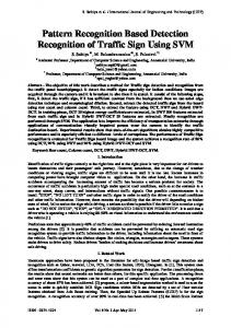
ASL is a complex visual-spatial language used by vocally or aurally disabled persons in the U.S. and Canada. ASL uses hand gestures, hand movements, or facial expressions to convey meanings such as the English Alphabet, numerals, colors, and so on. An ASL sign is a language unit in ASL, just like a letter or a word with specific meaning in English. According to ASL rules, there are no hand movements involved in most of the Alphabet letter signs; however, hand movements are required for representing ASL words and color signs. For example, color green is conveyed using hand shape of that of letter "G" with the wrist twisting twice; color yellow is conveyed using hand shape of that of letter "Y" with the wrist twisting twice, for more details, please refer to [2]. Our data are generated from a device called CyberGlove, which is a one-fits-all glove with 22 sensors located at different positions on a hand (see Figure 1). The sensor data measures the angle of joints at different parts of a hand, such as joints between the middle finger and the index finger, joints between a finger and the palm, and so on.
Figure 1: CyberGlove. Joint angles are measured at positions marked with a circle.
In addition to CyberGlove, there is a device called Polhemus Tracker, which can be located on the wrist to measure the hand position (in terms of values for X, Y, and Z coordinates relative to an initial setting) and the hand rotation (in terms of rotation of the palm plane to the X-Y, Y-Z and Z-X planes). The tracker generates 6 sensor values, values of X, Y, Z coordinates and angles of rotations relative the XY, Y-Z and Z-X planes. Effectively, the device software uses the various angles to model a human hand, and uses the tracker values to determine the hand motion trajectory; collectively the data from the 28 sensors capture the entirety of a hand motion. CyberGlove is used for many applications such as virtual reality, virtual classroom, and haptic applications. For the purpose of recognizing signs (or hand
motion patterns in general), we need to measure the similarity of different hand motions. As data from the sensors are continuously arriving; in our case the sensors generate data at a rate of about 100 Hz (i.e., 100 samples/second), data from each of the sensor can be considered as a CDS. At each sensor clock, which is about 0.01 second, the device software generates data for each of the 28 sensors, i.e., an array of 28 cells with each storing the value of one sensor at a given time, we call this one sample. The following is a sample taken from the data stream for color Orange: (-1.5116, -0.8463, -0.7278, 0.0693, -1.4068, -2.0700, -1.0193, 0.0042, -1.1508, -1.9977, -0.9374, 0.0003, -0.8039, -1.9847, -0.9231, -0.0161, -0.4424, -2.3644, -1.3870, -0.2155, -0.9737, 0.0146, 1.2882 -0.3191, 1.2383, -71.7795, 4.3214, 17.944) As time evolves, more and more samples are generated. We represent the data stream as a matrix, with the first sample as the first row, the second sample as the second row, and so on. This provides us with a matrix of 28 columns and multiple rows, the actual number of rows will depend on the time duration a hand motion lasts, e.g., if a hand motion lasts for t seconds, then the number of rows in the matrix will be roughly t × 100 . Before proceeding to describe our approach, we will survey studies related to our work in the next section. 3
Related Work
Query over CDS has been stimulating increasing interests in the database community lately. Most current research efforts are either on Database Management System (DBMS) support, such as Stream [3], Fjords [15], and NiagaraCQ [5], or on query processing and data mining issues, such as [6, 8, 9, 10]. Data sequences have been used in many applications, such as stock prices, biomedical measurements, weather data, DNA sequences, and sensor data from robotics. New emerging applications, such as data mining and information retrieval by content, require the capability of finding similar patterns, i.e., similarity query. Similarity query on persistent datasets has received a lot of attentions ([1, 4, 11, 12, 14, 17]), however to the best of our knowledge, there are no prior studies on pattern recognition/isolation over CDS. Clearly the performance of a similarity query (as component for pattern recognition) is determined largely by the chosen distance metric. The most straightforward approach for measuring the similarity between two sequences is to use a Minkowski measure such as the Euclidean distance. Given two sequences α = {x1 , x 2 ,..., xn } and β = { y1 , y 2 ,..., yn } , the distance between sequences α and
β
is defined as:
n
d (α , β ) = (∑ | xi − yi |2 )1/ 2 i =1
Euclidean distance metric is not suitable for our problem due to the effect of “dimensionality curse” and the requirement of identical length for the two sequences under investigation. Other approaches include DFT (discrete Fourier transform) [1] and DWT (discrete wavelet transform) [4], which are based on linear transformations and effectively treat a sequence with length l as a point in l -D space, and rotate the axes. This is exactly what singular value decomposition (SVD) does, but SVD does this in an optimal (in terms of L2 -norm) way for the given dataset; the reason is that effectively SVD maximizes the variance along the first few rotations [14] thus gives the optimal decomposition of the dataset by way of rotations. Furthermore, the nature of our data requires a 2-D transformation in case of DFT or DWT, however, since our datasets are not correlated on the sensor dimension at any given time, we do not expect DFT or DWT to perform well. These motivate us to use an SVD based approach. At the time of submission of this paper, we became aware of another related paper [22]. The problem studied in [22] is similar to ours in that both are trying to match the pattern currently in the data stream to a known set of time series (in our case, a set of predefined hand motions) and that patterns are of varying length. However, there are several differences between [22] and our work. The dataset in [22] is one dimensional, while our dataset is high-dimensional (28 D), which makes the problem more challenging due to the required tight aggregation and the impact of the 'dimensionality curse'. Therefore, our choice of weighted SVD for similarity measure is justified and of course different from the choice of Euclidean distance in [22]. Moreover, we deal with the real-time detection and separation of sequences, which has not been addressed in the past to the best of our knowledge. In [22], computation is always performed up to the current time and then the results are reported per each computation, in which case some of the results may not be very meaningful. Another novel aspect of our work is that we work on aggregated sensor streams. Finally, our application domain and datasets are unique. 4
Weighted-sum SVD
SVD is a numerically stable and efficient algorithm for computing singular values of a matrix. SVD is used extensively in statistical analysis (as the underpinning of the Principle Component Analysis) [13]. In database literature, SVD has been used primarily as a dimension reduction tool [14].
4.1
SVD Background
The idea of SVD is based on the following theorem of linear algebra [7]: Theorem If matrix and V such that
X ∈ R m×n , then there exist column-orthonormal matrices U
X = U × A ×V T m×r n×r r ×r Where U ∈ R and V ∈ R , and A ∈ R is a diagonal matrix A = diag (a1 , a2 ,..., ar ) such that a1 ≥ a2 ≥ ... ≥ ar . Each diagonal element in matrix A is the non-negative root of an eigenvalue of matrix X × X , and columns in matrix U are the corresponding eigenvectors. Geometrically, eigenvectors indicate rotations and the corresponding eigenvalue records the magnitude of rotations; or equivalently, we can view the different eigenvectors as the direction of projections, and the eigenvalues determines the strength of the projection on different directions. Effectively, SVD maximizes the variance along the first few dimensions. Figure 2 illustrates this effect by applying SVD to matrices of ASL color signs and some geometric shapes created by hand motions. T
(a) ASL color signs
(b) Geometric shapes Figure 2: Illustration of strength of rotations in different directions. The plot only shows values in the first ten most significant directions, the rest are omitted since they are extremely close to zero. The Xaxis indicates the indices of rotations towards different directions, while the Y-axis shows the corresponding rotation strength (which are actually singular values of the corresponding matrix). This figure shows that SVD maximizes the variance along the first few dimensions.
4.2
Weighted-Sum SVD as a Distance Metric
We now proceed to define the similarity metric for two data sequences. As described in Section 1, we use matrices M 1 and M 2 to represent two data sequences. Since the number of sensors is the same for all data sequences (28 in our case), the number of columns is fixed and identical for M 1 and M 2 , denoted by r ;
M 1 and M 2 need not be the same. Rather than defined directly on matrices M 1 and M 2 , our similarity metric is defined on their while the number of rows of
‘square’ matrices, i.e., on Q1 = M 1 × M 1 , and Q2 = M 2 × M 2 . This way the difference in the number of rows in the two matrices is taken care of. In fact, performing SVD on the ‘square’ of a matrix has been used extensively in computer vision and image processing literature ([16, 19, 20]). For ease of description, from now on we will not distinguish between a matrix and its square as well as singular values of a matrix and eigenvalues of the square of the matrix. Since ‘square’ matrices are symmetric, we have U = V . Consider for Q1 and Q2 , we have the following SVD decompositions: T
T
Q1 = V1 × A1 × V1
T
Q2 = V2 × A2 × V2
T
V1 and V2 are V1 = [e1 , e2 ,..., er ] and where V2 = [ f1 , f 2 ,..., f r ] , A1 = diag (c1 , c2 ,..., cr ) , A2 = diag (d1 , d 2 ,..., d r ) . The similarity of M 1 and M 2 is defined as:
Suppose columns representations of
θ ( M 1 , M 2 ) = min(θ1 ( M 1 , M 2 ),θ 2 ( M 1 , M 2 ))
(1)
Where r
r
i =1 r
i =1 r
θ1 ( M 1 , M 2 ) = (∑ ci (ei • f i )) /(∑ | ci |)
θ 2 ( M 1 , M 2 ) = (∑ d i (ei • f i )) /(∑ | d i |) i =1
and
i =1
x • y is the inner product of the two vectors x and y.
Intuitively, the above similarity metric compares the similarity along each projection directions. Moreover, as we perceive that projections along the directions with bigger strength should have more influence on the overall similarity of the two matrices, the overall similarity should be the weighted average of similarity along each projection directions where the eigenvalues serve as the weights of the corresponding projections. 5
The Ridge-Climbing Heuristic
In many applications, a continuous data stream may contain a series of data sequences with each encoding a particular meaning, and we wish to be able to separate the sequences from each other. There are two challenges for isolating the sequences: 1. 2.
The starting point for a sequence (except for the very first one) is not explicitly encoded in the data. Sequences encoding the same meaning may have varying lengths, this is because the amount of time it takes for different subjects to make the sign may not be exactly the same.
To address these problems, we propose a heuristic based on mutual information (for details on information theory, please refer to [18]). We define the signature of a sequence to be the SVD decomposition, i.e., the eigenvalues and the corresponding eigenvectors, of the matrix representing the target sequence. Assume we have precomputed the signature of a set of meaningful sequences termed our ‘vocabulary’, and assume all possible sequences that may occur in the data stream are from this set. We call any sequence from this set a reference sequence (or stream) and denote the vocabulary set as
S = {α1 , α 2 ,..., α n }
We define observation points as the time instances when we calculate the similarity between the data stream and some reference sequences. In our current setting, we compute similarity every 10 samples, which is roughly 0.1second as the frequency of our sensor device is about 100HZ. Let s denote the data stream, we are going to compute the similarity between
s and α i (i = 1,2,..., n) at observation
t = t0 < t1 < t2 < ... < t m , where the value m depends on the length of the sequence. Let θ ( s, α i , t ) denote the similarity between s and α i up to time t , clearly for fixed s and i , θ ( s,α i , t ) is a function of t and θ ( s, α i , t j ) ( j = 1,2,..., m) form a sequence. It is important to note that at each observation point t j , we consider the accumulated similarity values from t 0 to t j . Our heuristic point
is based on the following observation: Assume the sequence in stream sequence
θ ( s, β , t )
s that is to be detected is β ∈ S , then
(treated as function of t) is monotonically increasing up to
some time instance ξ and then starts decreasing. For this reason, we call our heuristic as the Ridge-Climbing Heuristic. Figure 3 shows the trend of accumulated similarity value changes at different observation points. We will model the relationship between the data stream and the reference sequence using information theory, in particular we will use the concept of mutual information. The following is an informal definition of mutual information [18]:
Figure 3: Trend of changes in similarity at different observation points. The data stream consists of color Black followed by color Blue and the reference sequence is color Black. The similarity keeps increasing, starting from t=0 until at around t=19 where a maxima is reached, then it starts decreasing. In the figure, ξ = 19 . From the trend of changes in similarity, we conclude that a switch to a new sequence happens at t=19, in the figure, the stream switches from black to the color blue.
Definition (Mutual Information) Let
α
β p{µ | ν } and
be two events, let
p{γ } denote
be the conditional probability of the probability that event γ occurs, let event µ with regard to event ν . Then the mutual information of α with respect to
β
is defined as following:
I (α ; β ) = log 2 ( p{α | β } / p{α }) Essentially I (α ; β ) indicates the amount of information gained for estimating
α
when β is known. The above definition for mutual information has the following nice properties: 1.
Symmetric
I (α ; β ) = I ( β ; α )
I (α ; β ) = 0 when α and β are independent This states that no information will be gained when an independent event is observed. Let si (i = 1,2,...) denote the samples occurring in stream s , we have the
2.
following Lemma:
Lemma Let
α i denote
i
event:
∏ k =1
{
sk is observed }, and assume β is the
sequence to be detected. To simplify our notation, we also use ^
s is observed if and only if s
^
is a sample and
β
to denote event: {
s occurs in β }. Thus, the ^
following result holds:
j , if i < j and all sk (1 ≤ k ≤ j ) occurs in β , then I ( β ; α i ) < I ( β ; α j ) .
1) Given i and
2) For any i , if si does not occur in β , then I ( β ; α i ) = −∞ . Proof. To avoid complicated mathematical argument, we shall use an informal proof. 1) Since
i < j , it follows that α j ⊂ α i , hence p{α j } ≤ p{α i } . Since all
sk ( 1 ≤ k ≤ j ) occurs in β , it is trivially true that p{α i | β } = 1 and p{α j | β } = 1. Using the fact that log 2 x is monotonically increasing for all x > 0, the following holds:
log 2 ( p{α i | β } / p{α i }) ≤ log 2 ( p{α j | β } / p{α j })
which is equivalent to say, 2) Since
I ( β ;α i ) < I ( β ; α j ) .
si does not occur in β , it follows that p{α i | β } = 0. However, p{α i } >
0, consequently I ( β ; α i ) = I (α i ; β ) = log 2 ( p{α i
| β } / p{α i }) = −∞
From 1) and 2), the result of the Lemma holds. The Lemma says that the mutual information keeps increasing before switching to a new sequence, and it then decreases. Intuitively, as the data stream carries information about the sequence to be detected, more information about the sequence is gained at the arrival of each new data sample. Since a similarity measure encodes a particular relationship between the data stream and the sequence to be detected, if the similarity measure is sensitive enough, it shall observe the monotonicity as stated in the Lemma. Through experiments, we see that the similarity metric defined in equation (1) satisfies this properly. Next, we describe an algorithm as well as a performance estimation analysis for implementing the above heuristic.
Procedure: Collect data for each of the possible vocabulary sequences dimension of samples in the sequence is Pre-compute SVD decomposition on Let
Q∈R i =1
r ×r
α1 , α 2 ,...,α N , the
r.
α1 , α 2 ,...,α N .
and initialize all its elements to zero
Let Loop
Collect
m samples
from the data stream, assume they form a matrix
M Let Let
T = MT ×M Q = Q +T
(2)
Q
SVD computation on For
i = 1 to N
θ (α i , Q) Keep track of all θ ’s for sequence α i Check whether θ ’s are monotonically increasing, and whether a Compute
maximum is reached (call this ‘switching criteria’) if the ‘switching criteria’ is satisfied place
αi
into the candidates pool
If window size is reached Choose from the candidate pool the maximal value, denote it as
αi
with biggest
αi0
Declare the stream so far observed to be sequence
αi0
Re-compute θ ’s for all sequences in the vocabulary since the time the new sequence starts Reset
Q
to be Null, plus some
R T × R , where R
consists all samples since the new sequence starts End
The window size in above procedure is determined so that we can unambiguously detect a sequence. The justification for Equation (2) is that, if matrix
[
]T
A can be written as A = B M , where M and B are matrixes with the same number of columns as A, and M is appended to the end of B in row-wise to generate A, then
AT × A = [B M ] × [B M ] = B T × B + M T × M T
Figure 4 illustrates the idea behind the above algorithm.
Figure 4: Sequence separation over CDS. The data stream consists of color Yellow, followed by Black, and Blue, similarity curves are generated for each of the three reference colors, Yellow, Black and Blue. The similarity curve between the data stream and Yellow keeps increasing from t=0 to t=30, it then starts decreasing, but we defer decision until around t=48, at which point we can unambiguously determine that the previous color is Yellow, and a new color occurs afterwards. 48 is the window size in this case, by looking back at the similarity curve, we know the color switch occurs at t=30, we reset the starting point of observation to be t0=30, and compute similarity values between the data stream and the three referenced colors, we observe that the similarity curve for color Black keeps increasing, and it has larger values than the other two curves, the increasing trend lasts until around t=50, at which point we see a decrease. At around t=78 (buffer size is 48) we make a decision that the previous color is Black, and the color switch occurs at around t=50, we reset t0 to be 50, and continue the detection.
Assume the size of the patter vocabulary is N , the number of sensors is r , the number of samples between consecutive observation points is m . The major computational cost of the above procedure comes from four sources, computation of
M T × M , computation of Q + T , computation of SVD on Q , computation of θ (Ci , Q) , which are O(mr 2 ) , O(r 2 ) , O(r 3 ) , and O(Nr ) respectively. Therefore,
the
total
cost
is
O (r × max(mr , r 2 , N )) . In our setting,
where r = 28, m = 10, N = 10 , the total cost is very reasonable, the computation can be computed well within the time limit of 0.1 second (the time duration between two consecutive observation points). Based on the computation cost estimation, we believe our procedure can accommodate N to as large as several hundred, which should be sufficient for detecting hand motion patterns.
6
6.1
Performance Evaluation
Experimental Setup
As described earlier, we use datasets from ASL color signs. We collected data from ten different persons, with each performing ten different color signs, i.e., black, blue, brown, green, grey, gold, orange, purple, red, and yellow multiple times. We then calculated the similarity between different colors. To represent each individual ASL color, we chose an aggregated data stream as representative for that particular color. For each color, there are several data streams generated by each of the ten different persons, a similarity matrix is then generated between each pair of the streams using the similarity metric defined by Equation (1). The data stream that has relatively higher similarity value was chosen as the representative data stream. For example, if we have the similarity matrix for streams A, B, C, D as shown in Table 1, then we would choose B as the representative stream. The decision was based on the average value at each row of the similarity matrix, the one with bigger values will be closer (more similar) to others; our experiments show that this simple method works well. In general, one can perform supervised clustering on a training set and use the centriods of the clusters as the representative streams. However, this was not the focus of this study. We store the SVD decomposition of the matrix for each representative as its signature. To obtain the trend of changes in similarity, we used data from ten subjects with each performing ten color sign combinations (such as Green-Orange, which means a user first performed a green color sign, and then changed to orange color sign), the computation (similarity at different observation points) was performed as the data were collected. Table 1: Mutual similarity matrix for streams A, B, C, and D. Each element in the table represents the similarity between the reference stream for the row and the reference stream for the column. For example, 0.3 in the last row records the similarity of stream C and D; 0.7 in the second row records the similarity of stream B and A.
A B C D 6.2
A 1.0 0.7 0.4 0.1
B 0.7 1.0 0.8 0.9
C 0.4 0.8 1.0 0.3
D 0.1 0.9 0.3 1.0
Experimental results
Table 2 shows the similarity values computed using similarity metric defined by equation (1):
Table 2: Similarity between colors yellow, orange, black, red, and green.
Yellow Orange Black Red Green
Yellow 0.965484 0.472714 0.427958 0.516680 0.480699
Orange 0.472714 0.946117 0.684033 0.546006 0.470286
Black 0.427958 0.684033 0.930344 0.896402 0.764338
Red 0.516680 0.546006 0.886402 0.960748 0.845138
Green 0.480699 0.470286 0.764338 0.845138 0.980830
Table 2 indicates that the similarity between the same colors is always significantly higher than that of different colors. Moreover, the colors that are more similar (in terms of hand motions) to each other have higher similarity values. For example, color signs Black and Red are similar in hand motions, and they have very high similarity value as shown in Table 2, also the similarity values between these two colors and other colors are quite close to each other; color sign Green and Orange are very different in hand motions, and the similarity value between these two colors is very small as shown in Table 2. This shows that our similarity metric is effective.
Figure 5: Curves for similarities computed at different observation points between the data stream and the sequence to be detected (Black, Yellow, Gold and Red in Black-Blue, Yellow-Black, Gold-Grey, Red-Yellow respectively). Black-Blue stream means a stream contains firstly data for Black color, followed by data for Blue color. The same is true for Yellow-Black stream, Gold-Grey stream, and RedYellow stream.
In Figure 5, each integer value on the X-axis corresponds to ten data samples, e.g., between 5 to 10 on the X-axis, there are 50 data samples. We can see that the similarity between the data stream and the sequence to be detected keeps increasing until reaching a maximum value, which is close to 1, then they start decreasing. This is consistent with the result of our Lemma. Intuitively, prior to determination of a sequence, more samples yield more information about the sequence under detection; when all samples have arrived, the sequence can be completely recognized, at which point the information derived from the data samples about the sequence shall be
maximal. Passing that point, samples from other sequences arrive, which do not contribute to the estimation of the original sequence, on the contrary, they appear to be noise and carry negative information about our original sequence. Figure 5 illustrates this observation. Another way to evaluate the performance of the heuristic is to see how well it performs when computing the similarity between the data stream and sequences not in the stream. Figure 6 shows similarities calculated between the data stream and some predefined patterns as more data samples are available, the similarities are calculated at individual observation points similar to Figure 3. In Figure 6, the
(a) Yellow-Black stream
(b) Black-Blue stream Figure 6: Trends of changes in similarity values between the data stream and some of the possible sequences. In (a), the data stream consists of color yellow followed by black; in (b) the data stream consists of color black followed by blue.
highest similarity value was observed for color yellow in a Yellow- Black stream until the switching point t = 30 and the same for color black in a Black-Blue stream until t = 20 , no other colors show better behaviors. Modeling similarity as mutual information as well as the informal proof for the Lemma did not take into account such factors as possible noise that may be present in the data and varying number of samples contained in a sequence; however, in practice, we observe the model as a good approximation and abstraction of the real scenario, which allows us to capture the essence of similarity measurement over CDS. 7
Conclusion and Future Plans
We proposed a similarity metric, weighted-sum SVD, to measure the similarity of immersive sequences occurring as continuous data streams (CDS). This has been done in the context of recognizing hand motions by analyzing the data streams collected from a virtual-reality glove. Our experiments with data generated by making ASL color signs show that the SVD metric performs well for sequence similarity measurement. Since our metric is SVD-based, it also handles challenges attributed to high dimensional spaces effectively. That is, measuring distances properly over the aggregation of 28-dimension sequences is a non-trivial task; however, weighted-sum SVD achieves this very well. Additionally, we proposed an information theoretic heuristic, the Ridge-Climbing Heuristic, for tackling the problem of sequence separation over continuous data streams. Our experiments demonstrate that modeling the similarity as mutual information is an appropriate mathematical abstraction. We plan to extend this study in two ways. First, we would like to explore techniques for computing SVD incrementally, i.e., computation of SVD utilizing results that have already been computed in the earlier steps thus reducing the overall computation cost considerably. Second, we intend to do a study to evaluate the effectiveness of different similarity metrics using our Lemma as a touchstone. 8
References
[1] R. Agrawal, C. Faloutsos, and A. Swami. Efficient similarity search in sequence databases. In Proc. of the 4th Intl. Conf. of Foundations of Data Organization and Algorithms, Chicago, 1993. [2] American Sign Language, http://dww.deafworldweb.org/asl/. [3] S. Babu and J. Widom. Continuous Queries Over Data Streams. ACM SIGMOD Record, 30(3), Sep. 2001.
[4] Kin-pong Chan, and A. Wai-chee Fu. Efficient time series matching by wavelets. ICDE 1999. [5] J. Chen, D. J. DeWitt, F. Tian, and Y. Wang. NiagaraCQ: A scalable continuous query system for internet databases. In Proc. of the ACM SIGMOD Conf. on Management of Data, May 2000. [6] J. Gehrke, F. Korn, and D. Srivastava. On computing correlated aggregates over continuous data streams. In Proc. of the ACM SIGMOD Conf. on Management of Data, May 2001. [7] G. H. Golub and C. F. van Loan. Matrix Computations. The John Hopkins Press, 1989. [8] S. Guha, N. Mishra, R. Motwani, and L. O’Callaghan. Clustering data streams. In Proc. of the 2000 Annual Symp. On Foundations of Computer Science. Nov. 2000. [9] M. R. Henzinger, P. Raghavan, and S. Rajagopalan. Computing on data streams. Technical Report TR-1998-011, Compaq Systems Research Center, Palo Alto, California, May 1998. [10] G. Hulten, L. Spencer, and P. Domingos. Mining time-changing data streams. In Proc. Of the 2001 ACM SIGKDD Int. Conf. On Knowledge Discovery and Data Mining, Aug. 2001. [11] P. Indyk, A. Gionis, and R. Motwani. Similarity Search in High Dimensions via Hashing. In Proc. of 25th International Conf. on Very Large Databases (VLDB), 1999. [12] H. V. Jagadish, A. O. Mendelzon, and T. Milo. Similarity Based Queries. In Symp. On Principles of Database Systems (PODS), 1995. [13] I. T. Jolliffe. Principal Component Analysis. Springer Verlag, 1986. [14] F. Korn, H. V. Jagadish, and C.Faloutsos. Efficiently supporting Ad Hoc queries in large datasets of Time Sequences. In Proc. of the ACM SIGMOD Conf. on Management of Data, 1997. [15] S. Madden and M. J. Frankin. Fjording the Stream: An Architecture for Queries over Streaming Sensor Data. ICDE Conference, San Jose, 2002. [16] H. Murakami and B. V. K. V. Kumar. Efficiently calculation of primary images from a set of images. IEEE T-PAMI, Vol. 4, No. 5, Sep. 1982. [17] S. Park, W. Chu, J. Yoon, and C. Hsu. Similarity Searches For Time-Warped Subsequences in sequence databases, ICDE 2000. [18] F. M. Reza. An Introduction to Information Theory, McGraw-Hill, 1961. [19] L. Sirovich and M. Kirby. Low dimensional procedure for the characterization of human faces. Journal of Optical Society of America, Vol. 4, No. 3, 1987. [20] M. Turk and A.Pentland. Eigenfaces for the recognition. Journal of Cognitive Neuralscience, Vol. 3, No. 1, Mar 1991. [21] C. Shahabi, G.Barnish, B.Ellenberger, N. Jiang, M. Kolahdouzan, A. Nam, and R. Zimmerman. Immersidata Management: Challenges in Management of Data
Generated within an Immersive Environment. Fifth International Workshop on Multimedia Information Systems (MIS), 1999. [22] L. Gao, X. Sean Wang. Continually Evaluating Similarity-Based Pattern Queries on a Streaming Time Series. In Proc. of the ACM SIGMOD Conf. on Management of Data, 2002. [23] C. Shahabi. AIMS: An Immersidata Management System. First Biennial Conference on Innovative Data Systems Research (CIDR’03), January 2003, Asilomar, CA.