PS2â©T (v) = w · sgn(PS2â©T (x)), PS2â©T (v)â ⤠w. The set of subgradients satisfying (4) is denoted by Sw(x). 2.1 Framework. We are concerned with signals ...
Recovery Threshold for Optimal Weight `1 Minimization Samet Oymak
M. Amin Khajehnejad
Babak Hassibi
Department of Electrical Engineering California Institute of Technology Pasadena, CA 91125 Abstract
We consider the problem of recovering a sparse signal from underdetermined measurements when we have prior information about the sparsity structure of the signal. In particular, we assume that the support of the signal can be partitioned into two known sets S1 , S2 where the relative sparsities over the two sets are different. In this situation it is advantageous to replace classical `1 minimization with weighted `1 minimization, where the denser support is given a larger weight. Prior work has analyzed the minimum number of measurements required for signal recovery with high probability as a function of the sizes of S1 , S2 , the sparsity levels and the weights. Numerical methods have also been devised to find the optimal weights. In this paper we give a simple closed form expression for the minimum number of measurements required for successful recovery when the optimal weights are chosen. The formula shows that the number of measurements is equal to the sum of the minimum number of measurements needed had we measured the S1 and S2 components of the signal separately. Our proof technique uses an escape through mesh framework and connects to the MMSE of a certain basis pursuit denisoing problem.
1
Introduction
Compressed sensing deals with the recovery of sparse signals from underdetermined observations [1]. In order to recover a k sparse signal x ∈ Rn from observations Ax ∈ Rm , a typical approach is minimizing the `1 norm of x subject to the constraints, i.e., min kˆ xk1 ˆ x
subject to Aˆ x = Ax (P 1)
In many cases, one might have extra information about the structure of the sparse signal x. In this paper, we will be considering a nonuniformly sparse model, where the signal is relatively sparser over region S1 and denser over the remaining region S2 = {1, 2, . . . , n} − S1 . Given this additional information, a reasonable approach to exploit this structure is to modify the regular This work was supported in part by the National Science Foundation under grants CCF-0729203, CNS0932428 and CCF-1018927, by the Office of Naval Research under the MURI grant N00014-08-1-0747, and by Caltech’s Lee Center for Advanced Networking.
`1 minimization algorithm. We will consider a regularized version of (P1) to tackle this problem. X X min |ˆ xi | + w |ˆ xi | s.t. Aˆ x = Ax (P 2) ˆ x
i∈S1
i∈S2
where w is the nonnegative weighting parameter. Problem Background: Weighted and reweighed algorithms has recently been subject of considerable interest. These problems have been investigated under various settings and interesting results have been provided which provably shows or argues by modifying regular `1 , substantial improvement in the recovery performance can be achieved [3–8]. Motivation and Contributions: An important performance criteria for a sparse recovery algorithm is its phase transition characteristics which is the relation between the sparsity k, ambient dimension n and number of measurements m. In this work, we investigate phase transitions of the regularized `1 minimization following the approach of [13]. Our motivation is to characterize the gain obtained by using optimal weighting for the problem (P2). We basically find out that, for optimal regularization w∗ , the number of required measurements for (P2) is equal to the total number of measurements, when the regions S1 , S2 are sensed separately and (P1) is used. This result is an interesting one as it provides a very simple connection between the regular `1 and optimally regularized `1 optimizations. Our result implies that although the information provided by Ax is a nontrivial mixture from regions S1 , S2 by using optimal weighting, one can do as good as if sensing x over S1 and S2 separately, i.e., as if A is a block diagonal matrix which doesn’t mix S1 and S2 . More accurately, let the size of the regions be |S1 | = n1 and |S2 | = n2 and sparsities be k1 , k2 . Given n and k, denote the “minimum number of measurements for successful recovery” (MoM) via (P1) by mn,k and denote the upper bound provided by our analysis by m ˆ n,k . Similarly, denote MoM for (P2) by mn1 ,k1 ,n2 ,k2 and our upper bound by m ˆ n1 ,k1 ,n2 ,k2 . In an asymptotic setting, we show that, m ˆ n1 ,k1 ,n2 ,k2 = (1 + o(1))(m ˆ n1 ,k1 + m ˆ n2 ,k2 ) (1) While this result is an equality of upper bounds, as a next step, we relate phase transitions obtained by our analysis to phase transitions of Approximate Message Passing (AMP) algorithms which is known to be same as the true phase transitions of `1 minimization, [12]. Using this we show, mn,k = m ˆ n,k (1 + o(1)) (2) This way, we provably show that optimally weighted `1 minimization is better or equal than separately measured two regular `1 minimization. We believe converse result is also correct as [19] experimentally shows m ˆ n1 ,k1 ,n2 ,k2 = mn1 ,k1 ,n2 ,k2 . As a side result, we provide the connection between AMP related works [10–12] and works that analyze the phase transitions for convex optimizations [13–17].
2
Problem Setup
Basic Definitions: Denote the set {1, 2, . . . , n} by [n]. Given T ⊆ [n], denote [n] − T by T¯. Further, we denote the operator that projects and collapse a vector on T by PT (·) : Rn → Rn and RT (·) : Rn → R|T | . In particular, PT (·) sets the entries over T¯ to 0 whereas RT (·) throws away the entries over T¯. Support T of a vector x is a subset of [n] such that it contains all the
nonzero locations, i.e., xi 6= 0 ⇐⇒ i ∈ T for all i ∈ [n]. sgn(·) : Rn → Rn is the function that x . returns entry-wise signs of a vector, i.e., 0 is mapped to 0 and x 6= 0 is mapped to |x| n Distance between two sets A, B ⊆ R is denoted by dist(A, B) and defined as minx∈A,y∈B kx−yk2 . Cone of a set A is denoted by cone(A). Given a scalar λ ≥ 0, denote the set obtained by scaling elements of a set A by λ by λ · A. Finally, for the rest of the discussion, we assume the regions S1 , S2 ⊆ [n] are fixed and known. Definition 2.1. Let x ∈ Rn be a vector with support T . Any subgradient v of the `1 norm at x has the following form, PT (v) = sgn(PT (x)), kPT (v)k∞ ≤ 1 (3) The set of vectors satisfying (3) is denoted by S(x). P P Similarly, let k · kw be the norm given as kxkw = i∈S1 |xi | + w i∈S¯i |xi |. Given x ∈ Rn with support T , any subgradient v of k · kw at x is of the form, PS1 ∩T (v) = sgn(PS1 ∩T (x)), kPS1 ∩T (v)k∞ ≤ 1 PS2 ∩T (v) = w · sgn(PS2 ∩T (x)), kPS2 ∩T (v)k∞ ≤ w
(4)
The set of subgradients satisfying (4) is denoted by Sw (x). 2.1
Framework
We are concerned with signals that have different sparsity levels over the regions S1 , S2 . The following definitions rigorize this notion. Definition 2.2 (Nonuniform Sparse Model). Given sets S1 , S2 = [n] − S1 and sparsities k1 , k2 , a signal x is called (|S1 |, |S2 |, k1 , k2 ) nonuniform. In particular, we will use a linear model where βi = nkii and αi = nni are constants for 1 ≤ i ≤ 2 and let n → ∞. Denote (α1 , α2 ) by α and (β1 , β2 ) by β. Then, we will simply say x is (α, β) nonuniform. A general signal with sparsity k = βn will similarly be called β sparse. Definition 2.3 (Minimum Number of Measurements). Let measurement matrix A ∈ Rm×n have i.i.d. standard normal entries. Given a signal s ∈ Rn that is β sparse, η(β) is the minimum number η so that, s can be recovered via (P1) asymptotically with high probability (w.h.p.) using m = (η + o(1))n measurements. Similarly, if s ∈ Rn is (α, β) nonuniform, η(α, β, w) is the minimum η so that s can be recovered from m = (η + o(1)) observations via (P2) w.h.p. Remark: It is known that, given k1 , k2 , n1 , n2 , for a Gaussian sensing matrix A, the required number of measurements for (P1) or (P2) is independent of locations or particular values of the nonzero entries, [2].
3
Main Results
Our main results can be summarized in two theorems. The first theorem is obtained by analyzing sharp upper bounds for phase transitions of (P1) and (P2), i.e., η(β) and η(α, β, w). In summary, we find, the number of measurements required to guarantee success in (P2) is equal to the total number required to guarantee success via (P1) as if the vectors RS1 (x) and RS2 (x) are measured separately. This statement is formalized below.
Theorem 3.1. Let g ∈ Rn be vectors with i.i.d. standard normal entries. Then, we have the following, • ηˆ(β) and ηˆ(α, β, w) are upper bounds to η(β) and η(α, β, w) and given as, ηˆ(β) = lim n−1 E[dist(g, cone(S(s1 )))]2 n→∞
(5)
ηˆ(α, β, w) = lim n−1 E[dist(g, cone(Sw (s2 )))]2 n→∞
where s1 , s2 represent β and (α, β) sparse vectors respectively. • Let ηˆ∗ (α, β) be the upper bound obtained by choosing the optimal regularization parameter w = w∗ that minimize ηˆ(α, β, w). Then, ηˆ∗ (α, β) = α1 ηˆ(β1 ) + α2 ηˆ(β2 )
(6)
The next result provides a connection between the upper bounds obtained in Theorem 3.1 and Approximate Message Passing (AMP) algorithms that are used for sparse recovery, [10–12]. To explain our approach, we first introduce the Basis Pursuit Denoising (BPDN) problem and its asymptotic minimum mean squared error (MMSE). Definition 3.1 (Basis Pursuit Denoising). Assume x ∈ Rn is a k sparse vector and we observe noisy vector y = x + z where z has i.i.d. Gaussian entries with variance σ 2 . We consider the following estimation problem, 1 ˆ k22 min λkˆ xk1 + ky − x ˆ x 2
(P 3)
It is known, [10], that E[kˆ x − xk22 ] is a function of k, λ, σ 2 . In the asymptotic setting where β = and n → ∞, we define optimally regularized normalized MMSE of BPDN to be, E[kˆ x − xk22 ] n→∞ λ≥0 σ→0 nσ 2
ηDN (β) = lim inf lim
k n
(7)
Our next result relates ηˆ(β) to ηDN (β) hence connects upper bounds obtained by Theorem 3.1 to BPDN. As it will be discussed soon, this will also imply ηˆ(β) = η(β). Theorem 3.2. ηˆ(β) is the same as given in (5), and ηDN (β) is as defined in Definition 3.1 and let g ∈ Rn be a vector with i.i.d. standard normal entries. Then, • For a β sparse vector s, ηDN (β) = lim n−1 inf E[dist(g, λ · S(s))2 ]
(8)
ηˆ(β) = ηDN (β) = η(β)
(9)
n→∞
λ≥0
• For any 0 ≤ β ≤ 1,
0.9 Weighted Algorithm (P2) Sum of Two Separate L1 Performance Gain Optimal Weight
0.88
η(α,β,w)
0.86
0.84
0.82
0.8
0.78
0.76 0
1
2
3
4
5
6
7
w (weight)
Figure 1: Blue line shows η(α, β, w) as a function of w for regularized `1 minimization. For this graph, we have α1 = 0.6, α2 = 0.4, β1 = 0.3 and β2 = 0.7. The green (straight) line shows the required measurements when regions are sensed separately. As predicted by Theorem 3.1, blue and green lines intersect at a single point. • Similar to ηˆ∗ (α, β) let η ∗ (α, β) be the amount of measurements for the optimally regularized (P2), i.e. minw≥0 η(α, β, w). Combining Theorem 3.1 and (9), η ∗ (α, β) ≤ ηˆ∗ (α, β) = α1 η(β1 ) + α2 η(β2 )
(10)
Comments about Theorems 3.1 and 3.2 • Observe that (10) implies that by using the optimal regularization, (P2) will asymptotically require less or equal measurements than the sum of two (P1)’s applied to S1 , S2 separately. • While we show ηˆ(β) = ηDN (β) in (9), ηDN (β) = η(β) is provided by [12]. The relation of BPDN and AMP has been studied in a series of papers including [10–12]. Denoting the asymptotic phase transitions of AMP by ηAM P (β), in [12], it has been shown that, ηAM P (β) = η(β) = ηDN (β)
(11)
• Our analysis are based on the strong concentration inequality given in Theorem 5.1 which is due to Gordon, [18]. By showing ηˆ(β) = η(β) = ηDN (β) we connect the series of papers that are based on Theorem 5.1 to results on AMP and BPDN [10–17]. In particular, (9) implies the results obtained by [13] are indeed tight and it is not surprising that it matches with exact phase transitions found in [2]. It also provides a strong justification for the tightness of the upper bounds in [14–17] for various sparse recovery problems including block sparsity and low rank recovery.
1
(measurements)
L1 phase transition Optimally Weighted L1
Improvement*
{
0.5
0 0
β1*
α1β1+α2β2*
0.5
β2*
1
Figure 2: The solid line is `1 phase transition. Dashed red line is the measurements required for optimally weighted (P2) as α1 , α2 varies and β1 , β2 are fixed.
4
Graphical Interpretation
Figure 1 illustrates an example setup where we set α = (0.6, 0.4) and β = (0.3, 0.7). Based on results of [5, 19], η(α, β) is plotted as a function of w. Green line corresponds to the sum of separate measurements. As expected from Theorems 3.1, 3.2, the relation η(α, β, w) ≥ α1 η(β1 )+ α2 η(β2 ) holds and equality is achieved for a particular w which is the optimal regularizer for (P2). Let us define the gain of the optimally weighted algorithm to be the reduction in the number of measurements compared to only applying (P1) or equivalently using w = 1. The gain, in Figure 1 is illustrated as the dashed line. In particular, Gain = η(α1 β1 + α2 β2 ) − η ∗ (α, β) = η(α1 β1 + α2 β2 ) − α1 η(β1 ) + α2 η(β2 )
(12)
Figure 2 provides a different view point for the improvement provided by optimally weighted (P2). The solid line is the phase transition η(β) of `1 minimization. Then, for fixed β1 , β2 , the dashed red line illustrates the required number of measurements as α1 = 1 − α2 varies. For example, α1 = 1 (P2) will need η(β1 ) measurements which is hardly surprising. The relation (6) can be translated as the linearity of the dashed line. Hence, the gain of the optimal weighting can again be characterized by (12) and it basically corresponds to the curvature of the η(·) function.
5
Analysis
Due to insufficient space we will be omitting most of the analytical derivations. Detailed derivations can be found in the Appendix. We begin by considering Theorem 3.1. The following section will describe our approach for this problem. 5.1
Proof Sketch of Theorem 3.1
We will make use of an approach that has been introduced in [13] and used in relevant works [14–17]. Definition 5.1. Let S ⊆ Rn and g ∈ Rn be a vector with i.i.d standard normal entries. Gaussian width of S is defined as, ω(S) = E[sup hv, gi] (13) v∈S
The next theorem provides a strong concentration result for random subspaces based on Gaussian width calculation. Theorem 5.1 (Escape Through a Mesh). Let S be a subset of unit ball B n−1 in Rn . Further, let H be an n − m dimensional subspace distributed uniformly over Grassmannian w.r.t Haar measure. Then, √ 1 P(H ∩ S = ∅) ≥ 1 − 3.5 exp(−( m − √ − ω(S))2 ) 4 m Based on Theorem 5.1, without losing generality, we will aim to obtain ηˆ(α, β, w). Let Mw (s2 ) be the set of vectors z such that ks2 + zkw ≤ ks2 kw . s2 is the unique optimal of (P2) if the null space N (A) of A and Mw (s2 ) have no intersection. N (A) is n − m dimensional uniformly distributed subspace due to Gaussianity of A. Hence, letting Sw = cone(Mw (s2 )) ∩ B n−1 and by making use of Theorem 5.1, s2 is the unique optimal w.h.p. if the number of measurements satisfies, √ 1 m − √ > ω(Sw ) (14) 4 m Following (14), ηˆ(α, β, w) provided by Theorem 5.1, takes a simple form. In particular, asymp2 totically ηˆ(α, β, w) = ω(Snw ) (1 + o(1)) will ensure success of (P2) w.h.p. Next, we cast the calculation of ω(Sw ) as the expectation of the following optimization problem where g is an i.i.d Gaussian vector with variance 1, max hg, zi
subject to
(15)
z ∈ cone(Mw (s2 )) and kzk2 = 1
(16)
z
Following [14], by writing and processing the dual problem and using convexity of Mw (s2 ), it can be shown that strong duality holds and the result of (15) is equal to, E[min kg − zk2 ] subject to z ∈ cone(Sw (s2 )) z
(17)
Observe that the final line is simply E[dist(g, cone(Sw (s2 )))] which yields, ηˆ(α, β, w) = n−1 E[dist(g, cone(Sw (s2 )))]2
(18)
to be a valid upper bound. ηˆ(β) can be found in a similar fashion. Next, let us consider the relation (6) of Theorem 3.1. Recall definitions introduced in Section 2. Let gi ∈ R|Si | be i.i.d. standard normal vectors for 1 ≤ i ≤ 2. Using (18) and making use of the structure of the sub-gradient of k · kw at nonuniform x, we have, (see Appendix), � � ηˆ(α, β, w) = n−1 E inf dist(RS1 (g), λ · S(RS1 (x)))2 + λ≥0 �1/2 �2 dist(RS2 (g), wλ · S(RS2 (x)))2 = n−1 E[inf (d1 (λ)2 + d2 (wλ)2 )1/2 ]2 λ≥0
(19)
where di (c) = dist(gi , cλ · S(RSi (x)))2 . We can similarly characterize α1 ηˆ(β1 ) and α2 ηˆ(β2 ). We have, αi ηˆ(βi ) = E[dist(gi , cone(S(RSi (x)))]2 = n−1 E[inf dist(gi , λ · S(RSi (x))]2 λ≥0
−1
= n E[inf di (λ)]2 λ≥0
(20) (21) (22)
Based on (19) and (22), what remains to show is whether, 2 X i=1
E[ inf di (λi )]2 ≈ E[inf (d1 (λ)2 + d2 (w∗ λ)2 )1/2 ]2 λi ≥0
λ≥0
(23)
for w∗ that minimizes right hand side of (19). Proof of (23) requires concentration inequalities for Gaussian vectors and is omitted here. In particular, our approach is based on the argument that, if the function sort(·) : Rn → Rn sorts the entries of a vector in an increasing order, and given i.i.d. standard normal g, if we let e ∈ Rn to be e = E[sort(g)] then sort(g) is concentrated around e. 5.2
Proof Sketch of Theorem 3.2
In order to estimate ηDN (β) we need to consider Definition 3.1. It is known that the optimal ˆ of (P3) is given as the shrinkage operator applied to y, [10–12]. solution x yi − λ if yi ≥ λ (24) xˆi = shrink(yi ) = 0 if |yi | < λ yi + λ else Let T denote the support of the sparse vector x. In the setting σ, λ → 0, for a Gaussian noise z, ˆ takes the following form, w.h.p. |xi | ≥ |zi | for all i ∈ T , and hence it can be shown that w.h.p. x ( xi + zi − λsgn(xi ) if i ∈ T xˆi = (25) shrink(zi ) else ˆ − x which can now be given as, Recall that we would like to characterize, x ˆ − x = PT (z − λsgn(x)) + PT¯ (shrink(z)) x
(26)
Keeping Definition 2.1 in mind, (26) simply reduces to, kˆ x − xk22 = σ 2 dist(g, λS(x))2
(27)
and hence, ηDN (β) = n−1 E[dist(g, λS(x))2 ]. Finally, we again make use of concentration results to show that this statement is equal to ηˆ(β) given in (22).
6
Further Directions
In this work, we have considered a nonuniform signal model where there are two distinct regions. In general, we believe it will not be hard to generalize results of this paper to a more St t general model with arbitrary number of regions {Si }i=1 , i=1 Si = [n] where we generalize (P2) to, t X X min wi |ˆ xj | s.t. Aˆ x = Ax (28) ˆ x
i=1 j∈Si
where w ∈ Rt is a noonegative weight vector. Such a model has actually been considered and analyzed in [5,19]. Based on the results of this work, denoting the normalized sizes and sparsities t of the regions by {αi }ti=1 , βi=1 , and denoting the number of measurements for optimally weighted ∗ t t (28) to be η ({αi }i=1 , {βi }i=1 ), it can be shown that, t X η ∗ ({αi }ti=1 , {βi }ti=1 ) = αi η(βi ) (29) i=1
Secondly, we believe weighted sparse recovery algorithms can be analyzed in a more general framework that is applicable to not only `1 minimization but also to closely related algorithms, such as `1 /`2 minimization and nuclear norm minimization, which are used for block sparse and low rank recovery. Finally, while we show that η ∗ (α, β) ≤ α1 η(β1 ) + α2 η(β2 ), the converse is only shown for the upper bounds ηˆ∗ (α, β). Consequently, it would be interesting to establish a deeper connection between our framework, which is based on Theorem 5.1, and results on Approximate Message Passing algorithms.
References [1] D. L. Donoho, “Compressed Sensing,” IEEE Trans. on Information Theory, 52(4), pp. 1289 - 1306, April 2006. [2] D. L. Donoho and J. Tanner, “Neighborliness of randomly-projected simplices in high dimensions,” Proc. National Academy of Sciences, 102(27), pp. 9452-9457, 2005. [3] N. Vaswani and W. Lu, “Modified-CS: Modifying compressive sensing for problems with partially known support,” IEEE Trans. Signal Processing, vol. 58(9), pp. 4595-4607, Sep. 2010. [4] L. Jacques, “A short note on compressed sensing with partially known signal support”, arXiv:0908.0660v2. [5] M. A. Khajehnejad, W. Xu, A. S. Avestimehr, B. Hassibi, “Weighted `1 minimization for sparse recovery with prior information,” Proc. Int. Symp. on Information Theory (ISIT) 2009. [6] T. Tanaka, J. Raymond, “Optimal incorporation of sparsity information by weighted `1 optimization,” Proc. Int. Symp. on Information Theory (ISIT) 2010. [7] W. Xu, M. A. Khajehnejad, S. Avestimehr, and B. Hassibi, “Breaking through the thresholds: an analysis for iterative reweighted `1 minimization via the Grassmann angle framework,” ICASSP 2010. [8] D. Wipf and S. Nagarajan, “Iterative Reweighted l1 and l2 Methods for Finding Sparse Solutions, IEEE J. Select. Topics Signal Process., vol. 4, no. 2, pp. 317329, 2010. [9] M. A. Khajehnejad, W. Xu, A.S. Avestimehr,and B. Hassibi, “Improved sparse recovery thresholds with two-step reweighted `1 minimization”, Proc. Int. Symp. on Information Theory (ISIT) 2010.
[10] D. L. Donoho, I. Johnstone and A. Montanari, “Accurate Prediction of Phase Transitions in Compressed Sensing via a Connection to Minimax Denoising”, available at arXiv:1111.1041v1. [11] D. L. Donoho, A. Maleki, and A. Montanari, “Message Passing Algorithms for Compressed Sensing”, Proceedings of the National Academy of Sciences 106 (2009), 18914-18919. [12] M. Bayati and A. Montanari, “The LASSO risk for gaussian matrices”, available at arXiv:1008.2581v1 [13] M. Stojnic, “Various thresholds for `1 - optimization in compressed sensing”, available at arXiv:0907.3666v1. [14] V. Chandrasekaran, B. Recht, P. A. Parrilo, and A. S. Willsky, “The Convex Geometry of Linear Inverse Problems” [15] N. Rao, B. Recht, and R. Nowak, “Tight measurement bounds for exact recovery of structured sparse signals”, arXiv:1106.4355, 2011. [16] M. Stojnic, “Block-length dependent thresholds in block-sparse compressed sensing”, arXiv:0907.3679v1. [17] S. Oymak and B. Hassibi, “New Null Space Results and Recovery Thresholds for Matrix Rank Minimization”, available at arXiv:1011.6326v1. [18] Y. Gordon, “On Milmans inequality and random subspaces which escape through a mesh in Rn ”, in Geometric Aspects of Functional Analysis, volume 1317 of Lecture Notes in Mathematics, pages 84-106. Springer, 1988. [19] A. Krishnaswamy, S. Oymak and B. Hassibi, “A Simpler Approach to Weighted `1 Minimization”, accepted to ICASSP 2012.
7 7.1
Appendix Concentration results for Gaussian vectors
Definition 7.1. Let abs(·) : Rn → Rn be the function that returns entry-wise absolute values of a vector. Similarly, let sort(·) : Rn → Rn be the function that sorts entries of a vector increasingly. ˜ = sort(abs(g)), i.e., the Let g ∈ Rn be a vector with i.i.d standard normal entries. Let g vector obtained by sorting absolute-valued g increasingly. g˜i = ith smallest absolute value in g
(30)
Finally, vector e = E[˜ g]. Observe that e is a function of n. Lemma 7.1. For any � > 0, there exists N such that for all n ≥ N , we have (1 − �) ≤
kek22 ≤1 n
(31)
Proof. For any i, ei = E[˜ gi ] =⇒ E[˜ gi2 ] ≥ e2i . Then using E[k˜ gk22 ] = E[kgk22 ] = n we find n ≥ kek22 . Left hand side of (31) is given in Section 7.2. Theorem 7.1. Assume n ≥ N as in Lemma 7.1. Then for any �0 > 0 √ √ P(k˜ g − ek2 ≥ ( � + �0 ) n) ≤ exp(−�20 n/2)
(32)
Proof. Lemma 7.2. k˜ g − ek2 is 1 Lipschitz function of g. Proof. Given, h and g we would like to show: ˜ − ek2 − k˜ |kh g − ek2 | ≤ kh − gk2
(33)
˜ − ek2 − k˜ ˜ −g ˜ k2 |kh g − ek2 | ≤ kh
(34)
From triangle inequality: Next, making use of Von Neumann’s trace inequality: ˜T g ˜ −g ˜ ≥ hT g =⇒ kh ˜ k22 − kh − gk22 ≤ 0 h
(35)
˜ −g ˜ k2 . Hence, kh − gk2 ≥ kh Now, using Gaussian concentration for Lipschitz functions we find √ P(k˜ g − ek2 ≥ E[k˜ g − ek2 ] + �0 n) ≤ exp(−�20 n/2)
(36)
What remains is to bound E[k˜ g − ek2 ]. Using E[˜ gi ] = ei and E[k˜ gk22 ] = E[kgk22 ] = n v v u n u n q q u X u X √ 2 2 2 2 t t E[k˜ g − ek2 ] ≤ E[k˜ g − ek2 ] = E[ (˜ gi − ei ) ] = E[ g˜i ] − kek = n − kek22 ≤ �n i=1
i=1
(37) 7.2
Left Hand Side of Lemma 7.1
Proof. Showing kek22 ≥ (1 − �)n for large n This is the more challenging part in the proof of Lemma 7.1. Let F (·) be distribution of absolute valued standard normal, F −1 (·) be inverse function of F (·), f (·) is the corresponding p.d.f. and f −1 (cdot)(x) is not the inverse function but simply 1/f (x). Lemma 7.3. 1/2 ≥ δ > 0, � > 0 can be arbitrarily small. Then, there exists an N = N (δ, �0 ) such that for any n > N all k such that k ≤ (1 − �0 )n satisfies ek ≥ F −1 (k/n) − δ
(38)
Proof. Let us estimate the deviation of g˜k from F −1 (k/n). In particular P(˜ gk ≤ F −1 (k/n) − �). Let x be a vector of random variables such that for all 1 ≤ i ≤ n ( 1 if |gi | ≤ F −1 (c) xi = (39) 0 else
P Let s = i xi . Clearly, s ≥ k ⇐⇒ |˜ gk | ≤ F −1 (c) hence P(s ≥ k) = P(˜ gk ≤ F −1 (c)). It is clear that xi ’s are i.i.d Bernoulli variables with P(xi = 1) = E[xi ] = c
(40)
Then, using a Chernoff bound, we can find P(˜ g(c+�)n ≤ F −1 (c)) = P(
X
xi ≥ (c + �)n) ≤ exp(−2�2 n)
(41)
i
Now, observing (F −1 )0 (x) = f −1 (x), which is increasing, we may write F −1 (x) ≤ F −1 (x − �) + �f −1 (x)
(42)
using a change of variable and letting k = (c + �)n we find P(˜ gk ≤ F −1 (k/n) − �f −1 (k/n)) ≤ P(˜ gk ≤ F −1 (k/n − �)) ≤ exp(−2�2 n)
(43)
Alternatively, P(˜ gk ≤ F −1 (k/n) − �) ≤ exp(−2�2 f 2 (k/n)n) ≤ exp(−2�2 f 2 (1 − �0 )n)
(44)
Denote, P(˜ gk ≤ x) by Fk (x) and Fk0 (x) by fk (x). Now, for any � > 0, we may write: Z
∞
xfk (x)dx ≥ (F
E[˜ gk ] =
−1
(k/n) − �)(1 − Fk (F
−1
Z
F −1 (k/n)−�
(k/n) − �)) +
xdFk (x)
(45)
0
0
Choosing � = δ/2 and letting n → ∞, we have Fk (F −1 (k/n)−�) → 0 hence E[˜ gk ] ≥ F −1 (k/n)−δ. Lemma 7.4. For any � > 0, there exists an N such that for all n > N we have kek22 ≥ (1 − �)n
(46)
Proof. Let h be a standard normal variable. Clearly, we have Z 1 Z ∞ 2 2 F −1 (x)2 dx 1 = E[h ] = x dF (x) = 0
(47)
0
Now, we choose three parameters that will be useful. • Choose an �0 so that Z
1
F −1 (x)2 dx < �/3
(48)
1−�0
• Secondly, choose δ = �/6. Then for any n > N (δ, �0 ), using Lemma 7.3, we may write X X kek22 ≥ e2k ≥ max{F −1 (k/n) − δ, 0}2 (49) k/n≤1−�0
k/n≤1−�0
Observe that max{F −1 (k/n) − �, 0}2 ≥ F −1 (k/n)2 − 2�F −1 (k/n).
• Finally, let N2 (�, �0 ) be such a number that for any n > N2 (�, �0 ) Z 1−�0 X −1 2 F −1 (x)2 dx ≥ (1 − �/3)2 n F (k/n) ≥ (1 − �/3)n k/n≤1−�0
X
(50)
0
F −1 (k/n) ≤ n
(51)
k/n≤1−�0
Note: We can make this assumption because from Riemann integration, as n → ∞ we have Z 1−�0 X −1 2 F −1 (x)2 dx (52) F (k/n) → n 0
k/n≤1−�0
X
F
−1
Z (k/n) → n
1−�0
p F −1 (x)dx ≤ n 2/π
Now assume n > max{N2 (�, �0 ), N (δ, �0 )}. Then we have X X e2k ≥ (F −1 (k/n)2 − 2�F −1 (k/n)) k/n≤1−�0
(53)
0
k/n≤1−�0
(54)
k/n≤1−�0
≥
X
F −1 (k/n)2 − 2δn
(55)
F −1 (k/n)2 − 2δn
(56)
k/n≤1−�0
≥
X k/n≤1−�0
≥ (1 − �/3)2 n − 2δn = (1 − 2�/3 + �2 /9 − �/3)n ≥ (1 − �)n
(57)
This completes proof of Lemma 7.1. 7.3
Identical Results
Assume α, β, S1 , S2 , T, w are as given previously. Definition 7.2. Let fw (·) : Rn → Rn be the function defined as follows: For 1 ≤ i ≤ 2: RSi ∩T (fw (x)) = sort(RSi ∩T (x)) RSi ∩T¯ (fw (x)) = sort(abs(RSi ∩T¯ (x)))
(58) (59)
Further, let fi (·) : Rn → Rni such that: fi (x) = RSi (f (x))
(60)
One may show the following results which are identical to Lemma 7.1 and Theorem 7.1. Proof is omitted as it follows the exact same steps.
Lemma 7.5. Assume g ∈ Rn is a vector with i.i.d. standard normal entries. Let e = E[fw (g)], ei = E[fi (g)]. Then, for any � > 0, there exists an N (�) such that any n > N (�), we have: (1 − �)n ≤ kek22 ≤ n (1 − �)ni ≤ kei k22 ≤ ni , 1 ≤ i ≤ 2
(61) (62)
Combining, Lemma 7.5 and Lipschitzness of fw (·), fi (·), we may obtain the following. Theorem 7.2. Assume g ∈ Rn . Then there exists a constant c = c({αi }, {βi }) > 0 such that for any n > N (�), �0 > 0, √ (63) P(kfw (g) − ek2 ≥ (� + �0 ) n) ≤ exp(−c�20 n) √ 2 P(kfi (g) − ei k2 ≥ (� + �0 ) ni ) ≤ exp(−c�0 ni ) (64) 7.4
Proof of Theorem 3.1
We first argue that (15) and (17) are equivalent. This follows from the fact that “polar cone” of cone(Mw (s2 )) is simply the cone of sub-gradients of k · kw at s2 , i.e., cone(Sw (s2 )). Reader is referred to [14] for the detailed arguments and a more general setup in which various phase transitions are analyzed based on Theorem 5.1. Now, we will focus on showing (6). In order to simplify our discussion, without loss of generality, [2, 13], we’ll assume x is nonnegative hence for any nonzero xi , sgn(xi ) = 1. Continuing from Section 5.1, observe that we need to show (23). Let us first observe the following. Lemma 7.6. Let v ∈ Rn be an arbitrary vector. Assume x ∈ Rn obeys the nonuniform model and Sw (x), S(RS1 (x)) and S(RS2 (x)) are same as in Section 5.1. Then for any λ > 0, dist(v, λ · Sw (x)) = dist(fw (v), λ · Sw (x)) dist(RSi (v), λ · S(RSi (x))) = dist(f (RSi (v)), λ · S(RSi (x))))
(65) (66) (67)
Proof. This follows from the following property of `1 and weighted `1 norms. For example, for k · kw norm, the minimum distance is `2 norm of v ˆ which can be found coordinate wise as follows: vi − λ if i ∈ S1 ∩ T shrink(v ) if i ∈ S ∩ T¯ i 1 vˆi = (68) v i − wλ if i ∈ S2 ∩ T w · shrink(vi /w) if i ∈ S2 ∩ T¯ Call, w = fw (v). Now, observe that fw (·) simply permutes the elements of a vector on the sets ˆ and v Si ∩ T hence w ˆ is same over Si ∩ T up to permutation. Finally, observe that for any ˆ and v number, |shrink(c)| = |shrink(−c)| hence over Si ∩ T¯, magnitudes of w ˆ are same up to ˆ 2 = kˆ permutation. Overall, kwk vk2 as desired. Following lemma will be critical to subsequent analysis.
Lemma 7.7. Let g be an i.i.d. standard normal vector and assume e, e1 , e2 are same as in Lemma 7.5. Further, let: cw = min dist(e, λSw (x))
(69)
ci = min dist(ei , λS(RSi (x))), 1 ≤ i ≤ 2
(70)
λ≥0
λ≥0
Then, for any � > 0: √ |E[dist(g, cone(Sw (x)))] − cw | ≤ � n
√ |E[dist(RSi (g), cone(S(RSi (x))))] − ci | ≤ � n
(71) (72)
For sufficiently large n. Proof. For simplicity, denote cone(Sw (x)) by S. WLOG, we’ll show the result for cw , Sw (x). We know that: E[dist(g, S] = E[dist(fw (g), S)] (73) Next, we can write: dist(e, S) − E[dist(fw (g) − e, S)] ≤ E[dist(fw (g), S)] ≤ dist(e, S) + E[dist(fw (g) − e, S)] (74) We also know dist(e, S) = cw . Hence: |E[dist(fw (g), S] − cw | ≤ E[dist(fw (g) − e, S)]
(75)
We need to find a good bound for the right hand side. We will first use: E[dist(fw (g) − e, S)] ≤ E[kfw (g) − ek2 ]
(76)
Now, we can make use of the fact that kfw (g) − ek2 is concentrated somewhere around 0, i.e. for sufficiently large n and any �, �0 > 0, based on Theorem 7.2: √ (77) P(kfw (g) − ek2 ≥ (�/2 + �0 ) n) ≤ exp(−c�20 n) √ Now, with standard arguments, (integration by parts), it can be shown that E[|fw (g)−ek2 ] ≤ � n for sufficiently large n. Next theorem, concludes the proof of Theorem 3.1 by showing ηˆ∗ (α, β) = α1 ηˆ(β1 ) + α2 ηˆ(β2 ). Theorem 7.3. Let g ∈ Rn be an i.i.d. standard normal vector. For any � > 0 and for sufficiently large n and for the optimal choice of weight w∗ , we have: 2
|E[dist(g, cone(S (x)))] − w∗
2 X
E[dist(RSi (g), cone(S(RSi (x)))]2 | ≤ �n
(78)
i=1
Consequently, letting n → ∞: ηˆ∗ (α, β) =
2 X i=1
αi ηˆ(βi )
(79)
Proof. To show the result, we make use of the previous lemma. Using Lemma 7.7, for any δ > 0, for arbitrarily large n we have: |E[dist(g, cone(Sw (x)))]2 − c2w | ≤ δn |E[dist(RSi (g), cone(S(RSi (x))))]2 − c2i | ≤ δn
(80) (81)
From these, it can be observed that, we simply need to argue that minw c2w = c2w∗ = c21 + c22 . Let λ1 , λ2 denote the particular values that achieve: min dist(ei , λS(RSi (x))), 1 ≤ i ≤ 2
(82)
λ≥0
Step 1: Observe that, for any choice of w and λ, we have: dist(e, λSw (x))2 = dist(e1 , λS(RS1 (x)))2 + dist(e2 , λwS(RS2 (x)))2 ≥ c21 + c22
(83)
Hence, minimizing the left hand side of (83) in terms of λ and w, we obtain c2w∗ ≥ c21 + c22 . Step 2: Conversely, choosing w = λλ12 we are achieving equality in (83) hence we have c2w∗ ≥ c21 + c22 . Combining these, we achieve c2w∗ = c21 + c22 . Consequently, we obtain: 2
|E[dist(g, cone(Sw (x)))] −
2 X
E[dist(RSi (g), cone(S(RSi (x))))]2 | ≤ 3δn
(84)
i=1
On the other hand, information theoretic lower bound on sparse recovery will yield (to recover a k sparse vector we need at least k measurements): 2
E[dist(g, cone(Sw (x)))] ≥ n
2 X
αi βi
(85)
i=1 2 X
2
E[dist(RSi (g), cone(S(RSi (x))))] ≥ n
i=1
2 X
αi βi
(86)
i=1
Combining the fact that n
P2
i=1
αi βi � 3δn, and letting δ → 0, we can conclude: 2
X E[dist(g, cone(Sw (x)))]2 → 1 =⇒ ηˆ∗ (α, β) = αi ηˆ(βi ) P2 2 E[dist(R (g), cone(S(R (x))))] S S i i i=1 i=1
7.5
(87)
Proof of Theorem 3.2
This part of the proof will require perturbation analysis. First, let us consider the shrink(·) function and show the following. Lemma 7.8. Consider the denoising setting. y = x + z where z, g are i.i.d. Gaussian vectors ˆ = shrink(y) is the output of LASSO, where shrink is same as with variance σ 2 , 1 respectively. x in Section 5.2. Then, assuming λ → 0 as σ → 0: lim σ −2 E[kˆ x − xk22 ] → E[dist(g, λσ −1 S(x))2 ]
σ→0
(88)
Proof. Similar to `1 recovery problem, WLOG, x can be assumed nonnegative, [12]. In particular, we assume this to simplify the notation. First, we may write: E[kˆ x−
xk22 ]
=
n X
E[(ˆ xi − xi )2 ]
(89)
i=1
For i ∈ T¯, we have xˆi − xi = shrink(zi ) hence using RT¯ (x) = 0: X E[kshrink(RT¯ (z))k22 ] = σ 2 E[dist(RT¯ (g), λσ −1 S(RT¯ (x)))2 ] E[kRT¯ (ˆ x − x)k22 ] =
(90)
i∈T¯
Hence, what remains is dealing with in support terms. To do this, we’ll simply show for i ∈ T : lim σ −2 E[(shrink(yi ) − xi )2 ] → E[(gi − σ −1 λ)2 ]
σ→0
(91)
Recalling the definition of shrinkage operator given in Section 5.2, observe that |shrink(yi )−xi | ≤ |zi − λ| in all cases. Hence, LHS of (91) is upper bounded by E[(gi − σ −1 λ)2 ]. Next, we’ll argue that as σ → 0, upper bound is achievable. We may write: Z ∞ Z 2 2 E[(shrink(yi ) − xi ) ] = (shrink(xi + zi ) − xi ) p(zi )dzi ≥ (zi − λ)2 p(zi )dzi (92) −∞
zi ≥λ−xi
Now, since λ, σ → 0 and xi is a positive constant, distribution of zi will almost fully lie between [λ − xi , ∞) hence: Z −2 lim σ (zi − λ)2 p(zi )dzi = E[(zi − λ)2 ] = E[(gi − σ −1 λ)2 ] (93) σ→0
zi ≥λ−xi
= E[dist(RT (g), λσ −1 S(RT (x)))2 ]
(94)
In general, it is not difficult to show that optimal regularizer λ∗ will approach 0 as σ → 0 hence, based on Lemma 7.8, we obtain: ηDN = lim min n−1 E[dist(g, λS(x))2 ] n→∞ λ>0
(95)
Finally, in order to show ηDN = ηˆ, we make use of the following theorem. Theorem 7.4. For any � > 0, there exists N (�) such that any n > N (�), we have: | min E[dist(g, λS(x))2 ] − E[dist(g, cone(S(x)))]2 | ≤ �n λ>0
Hence, letting n → ∞, � → 0, we obtain ηDN = ηˆ.
(96)
Proof. The proof will make use of the same technique used in Lemma 7.7. Use the function fw (·) with w = 1 and set e = E[fw (g)]. We know, E[dist(g, λS(x))2 ] = E[dist(fw (g), λS(x))2 ] E[dist(g, λS(x))]2 = E[dist(fw (g), λS(x))]
(97) (98)
and we further know, dist(fw (g), λS(x)) concentrates around dist(e, λS(x)) for large n. From the proof of Lemma 7.7, it is known that: min dist(e, λS(x))2 ≈ E[dist(g, cone(S(x)))]2 λ>0
(99)
For minλ>0 E[dist(g, λS(x))2 ] we may first write: min E[dist(g, λS(x))2 ] ≥ min E[dist(g, λS(x))]2 ≈ min dist(e, λS(x))2 λ>0
λ>0
λ>0
(100)
To find an upper bound on the√left hand side of (100) use λ∗ that minimizes minλ>0 dist(e, λS(x)). Use dist(e, λS(x)) ≤ kek2 ≤ n and call a = dist(e, λ∗ S(x)), b(g) = dist(fw (g), λ∗ S(x)). Using Theorem 7.2 and |a − b(g)| ≤ ke − fw (g)k2 , we have the following concentration for �0 > 0: √ P(|a − b(g)| > (� + �0 ) n) ≤ exp(−c�20 n) (101) Writing b(g)2 − a2 = (b(g) + a)(b(g) − a) ≤ 2a(b(g) − a) + (b(g) − a)2 , we may proceed as follows: √ (102) E[2a(b(g) − a)] ≤ 2 nE[b(g) − a] (101) shows b(g) − a is concentrated around 0 (for small �). Hence, for sufficiently large n, A simple integration by parts will show: √ E[b(g) − a] ≤ 2� n =⇒ E[2a(b(g) − a)] ≤ 2�n (103) Similarly, for (b(g) − a)2 , (101) gives for �0 > 0: P((a − b(g))2 > (� + �0 )2 n) ≤ exp(−c�20 n) Let t =
|a−b(g)| √ . n
(104)
Hence, denoting 1 − c.d.f. of t by Q(·), we may write: −1
2
2
Z
∞
x2 dQ(x) 0 Z ∞ 2 ∞ = −[Q(x)x ]0 + 2xQ(x)dx
n E[(a − b(g)) ] = E[t ] = −
(105) (106)
0
Not that −[Q(x)x2 ]∞ 0 = 0 and for the other term, using �0 = x − � we have: Z ∞ Z 0 Z ∞ 2xQ(x)dx ≤ 2(� + �0 )Q(� + �0 )d�0 + 2(� + �0 ) exp(−c�20 n)d�0 0
−�
0
(107)
Z
0
Z
0
2(� + �0 )Q(� + �0 )d�0 ≤ −�
2�d�0 = 2�2
(108)
−�
As n → ∞, remaining term on the right hand side will clearly approach 0 as tail of the exponential becomes heavier. For example: Z ∞ Z ∞ 1 1 2 2�0 exp(−c�0 n)d�0 = d exp(−c�20 n) = (109) cn 0 cn 0 and Z 0
∞
2� exp(−c�20 n)d�0
r π =� cn
(110)