Redalyc.DESIGN AND IMPLEMENTATION OF AN

Redalyc Scientific Information System Network of Scientific Journals from Latin America, the Caribbean, Spain and Portugal

ESCOBAR JIMÉNEZ, RICARDO FABRICIO; ASTORGA ZARAGOZA, CARLOS MANUEL; HERNÁNDEZ, JOSÉ A.; MEDINA, MANUEL ADAM; GUERRERO RAMÍREZ, GERARDO VICENTE DESIGN AND IMPLEMENTATION OF AN OBSERVER-BASED SOFT SENSOR FOR A HEAT EXCHANGER Dyna, vol. 78, núm. 166, abril-junio, 2011, pp. 89-97 Universidad Nacional de Colombia Medellín, Colombia Available in: http://www.redalyc.org/src/inicio/ArtPdfRed.jsp?iCve=49622365012

Dyna ISSN (Printed Version): 0012-7353 [email protected] Universidad Nacional de Colombia Colombia

How to cite

Complete issue

More information about this article

Journal's homepage

www.redalyc.org Non-Profit Academic Project, developed under the Open Acces Initiative

DESIGN AND IMPLEMENTATION OF AN OBSERVER-BASED SOFT SENSOR FOR A HEAT EXCHANGER DISEÑO E IMPLEMENTACIÓN DE UN SENSOR VIRTUAL BASADO EN OBSERVADOR PARA UN INTERCAMBIADOR DE CALOR RICARDO FABRICIO ESCOBAR JIMÉNEZ Centro Nacional de Investigación y Desarrollo Tecnológico, Cuernavaca Morelos, México, [email protected]

CARLOS MANUEL ASTORGA ZARAGOZA Centro Nacional de Investigación y Desarrollo Tecnológico,Cuernavaca Morelos, México, [email protected]

JOSÉ A. HERNÁNDEZ Centro de Investigación en Ingeniería y Ciencias Aplicadas – Universidad Autónoma del Estado de Morelos, Cuernavaca, Morelos, México., [email protected]

MANUEL ADAM MEDINA Centro Nacional de Investigación y Desarrollo Tecnológico,Cuernavaca Morelos, México, [email protected]

GERARDO VICENTE GUERRERO RAMÍREZ Centro Nacional de Investigación y Desarrollo Tecnológico, Cuernavaca Morelos, México, [email protected] Received for review October 30 th, 2009, accepted October 8th, 2010, final version October, 22 th, 2010

ABSTRACT: The objective of this work is to describe step-by-step how to implement an observer-based soft sensor in order to estimate process variables for which a hardware sensor is not available. The design and implementation procedure is illustrated by applying it to a counter-flow double-pipe heat exchanger. The approach used to design the nonlinear observer is based on a simplified mathematical model of the process. Numerical simulations and experiments were performed in a bench-scale pilot plant in order to validate the proposed scheme. KEYWORDS: Soft sensor, nonlinear observer, heat exchanger. RESUMEN: El objetivo de este trabajo es describir paso a paso la implementación de un sensor basado en observador para estimar las variables de un proceso para el cual no existe la disponibilidad de un sensor físico. El procedimiento de diseño e implementación se ilustra mediante su aplicación a un intercambiador de calor de doble tubo con flujos a contracorriente. El enfoque empleado para diseñar el observador no lineal se basa en un modelo matemático simplificado del proceso. Se desarrollaron simulaciones numéricas y posteriormente pruebas experimentales en una planta piloto (intercambiador de calor) con el fin de validar el esquema propuesto. PALABRAS CLAVE: Sensor virtual, observador no lineal, intercambiador de calor.

1. INTRODUCTION

observer is the main mathematical tool which makes the conception of a soft sensor possible.

SOFT sensors are an alternative to estimate process variables [1-2]: they can be used to replace costly sensors. A soft sensor can be defined as the association between a hardware sensor and an estimation algorithm as shown in Fig. 1 and studied by Farza et. al. in [3]. The estimation algorithm (also called state observer in this context) is the software part which performs the on-line estimation of the process variables using the available measurements. Therefore, a state Figure 1. Principle of an observer-based soft sensor Dyna, Year 78, Nro. 166, pp. 89-97. Medellin, April, 2011. ISSN 0012-7353

90

Escobar et al

State observers have been studied since 1960. The works developed by Kalman in [4] and by Luenberger in [5] solve the problem of state estimation for linear systems [26]. The property of observability, characterized by the rank condition guarantees the possibility of indeed designing an observer. In the nonlinear case, the observability depends on the input of the system. In this case, the observability of a nonlinear system does not exclude the existence of singular inputs (inputs for which two distinct initial states cannot be distinguished by using the known measured output). There are several approaches to designing nonlinear observers; these depend on the specific structure of the system to be observed [6-9, 27]. For instance, in Gauthier et. al. [6] high-gain observers have been used to estimate the states of control-affine nonlinear systems; Targui et. al. [7] proposed a nonlinear observer for a particular class of nonlinear systems which have a triangular structure; Besançon et. al. [8] present in their work an adaptive observer for state-affine nonlinear systems; while Gauthier and Kupka [9] proposed an observer for systems having the nonlinear general form dx / dt  f  x  . The main purpose of this paper is to describe step-bystep how to implement a nonlinear observer in order to develop a soft sensor for a heat exchanger. This kind of real-time control laboratory allows both, process engineers and students of control systems to visualize the fact that a soft sensor represents a viable alternative to avoid unnecessary, expensive instrumentation in a process.

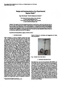
2. PROBLEM STATEMENT A double-pipe heat exchanger, Fig.2 (formed by two concentric tubes) can be operated in parallel (the fluids flow in the same direction through the inner and the outer tubes) or in counter-flow mode (the fluids flow in opposite directions). In this study, the second case is considered. The main process variables of this kind of processes are: the inlet temperature of the fluid in the hot side Thi , the inlet temperature of the fluid in the cold side Tci , the outlet temperature of the fluid in the hot side Tho , the outlet temperature of the fluid in the cold side Tco , the flow rate in the hot side vh and the flow rate in the cold side vc . The instrumentation diagram of a double-pipe heat exchanger pilot-plant developed by Didatec Technologies is shown in Fig. 3. The plant operates as a water-cooling process: the hot water flows through the inner tube and the cooling water flows in the shell (the external tube). The pilot-plant is equipped with the following instruments: Tci and Tco are measured via two SIKA® glass thermometers (TI1 and TI2 respectively); Tco and Thi are measured via two Engelhard Pyro-Controle Pt-100 temperature transmitters (TT1 and TT2 respectively); vc and vh are measured by means of two Platon variable section flowmeters (FI1 and FI2 respectively).

Figure 3. Instrumentation diagram of the counter-flow double-pipe heat exchanger

Figure 2. Counter-flow double pipe heat exchanger

Let’s suppose that a state-feedback control law is needed to control the outlet temperatures [10]. It is well known that this kind of control requires

91

Dyna 166, 2011

the on-line measurement of the states of the whole process. In the Didatec Technologies pilot-plant this is not possible because the state variable Tho is not measured electronically; so, it cannot be used for feedback control purposes. Another useful application is a remote monitoring system for whole process states. In the current configuration, the operator of the plant would have to move to the place where the thermometer is installed to be able to take the corresponding measurement.

The heat exchanger can be divided into small elements called cells, every cell consisting of two stirred tanks as shown in Fig. 4. The model equations for a single cell are deduced from energy and mass balances for the cold and hot side.

These two problems (control and monitoring) can be solved by designing a soft sensor. The approach used to design the soft sensor is described as follows: S1: Select or develop an adequate mathematical model of the process. S2: Select an adequate observer depending on the model structure. S3: Design and program the observer in order to make numerical simulations tests. S4: Implement the observer in a computer-based system following the scheme shown in Fig.1. The above steps of the approach are developed in the following sections.

Figure 4. One-cell representation of a double-pipe heat exchanger

Before presenting the mathematical model, the following assumptions should be introduced: A1: Adiabatic operation.

3. STEP 1: HEAT EXCHANGER MATHEMATICAL MODEL

A2: The inlet temperatures Tci and Thi are known.

Distributed parameter models are those that best fi t to the nature of heat exchangers [11], however this kind of model is often difficult to analyze or to use with feedback [10]. One of the models which can be used for control purposes is presented by Fazlur and Devanathan [12].

A4: The physical and chemical properties of the fluids are constant.

With this approach, the heat exchanger model can be seen as a gray box in which some lumped parameters are considered in order to simplify the whole model. Zavala-Río and Santiesteban-Cos [13] demonstrated the qualitative equivalence between the distributed-parameter models and the lumped models. Specifically, three aspects were proven to be shared by both models: existence and uniqueness of solutions, equilibrium states, and stability properties. The authors in [14], [15] used lumped-parameter models in order to conceive a fault diagnosis system for heat exchangers. In both cases the results obtained using models considering a spatial discretization of the process were acceptable.

A3: The inlet temperatures Tci and Thi are constant.

A5: The global heat transfer coefficient U is constant. Under the assumptions A1-A4, and considering an energy balance law for every cell, the single-cell heat exchanger model is given by:

2   Tco  V  c  T  2  ho Vh

v T  T  UAT  c  ci co  Cpc

 c 

v T  T  UAT  h  hi ho  Cph

 h 

(1)

A complete discussion about modeling heat exchangers can be found in [12, 16, 17], where is the (mean) temperature difference among the fluids. Basically, there are three approaches proposed in the literature for : T  Tho  Tco i) the temperature difference .

92

Escobar et al

ii) the arithmetic mean temperature difference (AMTD) defined as T 

1 2

 T

ho

 Tci    Thi  Tco 

,

iii) he logarithmic mean temperature difference (LMTD) defined as T 

 T  T    T  T   ln T  T ) / (T  T )  . ho

ho

ci

hi

ci

co

hi

co

See [18] for further information. Zavala-Río and Santiesteban-Cos [13] proved that the use of the logarithmic mean temperature difference approach (also known as the LMTD driving-force) provides reliable dynamic representations for heat exchangers especially in cases where it is not the quantitative solutions but the qualitative behavior that is important. The LMTD driving-force is expressed in a simplified form as     T2  T1   T   T  ln  2    T  1  

High-gain observers work either for autonomous systems or for nonlinear systems that are observable for each input. One of the main features of these observers is that they are easy to implement, because the observer gain is obtained from an algebraic Lyapunov equation and is simple to compute. Highgain observers have been applied to several kinds of processes, i.e. polymerization reactors [24], distillation columns [7], and chemical reactors [25]. For these reasons (implementation and tuning facilities), in the following sections, the high-gain observer is used to design the soft sensor for the heat exchanger. 4.1 The high-gain observer The control-affine nonlinear system is given by:

(2)

Where T1  Thi  Tco  and T2  Tho  Tci  Equation (2) has a numeric indetermination when T1  T2 generally in the initial condition T0 for this reason a modified LMTD model is introduced to express the temperature difference :

 T2  T1  T2  T1  T  ln  2 T    T1    T0 T2  T1 

Kalman observers have been used successfully for several processes (see for instance [21-22]), it is well known that technically they are difficult to implement and difficult to tune, this is because a Riccati equation must be solved and a numerical instability can easily arise due to the accumulated errors [23].

 x  f  x    m ui gi  x  i 1  y  h x   

n where x   , ui   , y   , f  x    n and g i   Assume that the system in (4) is observable and consider the nonlinear change of coordinates of T z    x  where   x    h  x  L f h  x  Lnf1h  x   The notation L f   represents the Lie derivative of a real valued function along f  x  . By definition

n

(3)

(4)

L f   h  x    i 1

h  x  fi  x  xi

(5)

The analytical properties of the LMTD model in (3) are reported in [13].

the transformation   x  determines a system which takes the form

4. STEP 2: OBSERVER SELECTION

 z  Az    y  Cz

The most-widely known observers in the literature are the extended Kalman observers (also known as extended Kalman filters) [1, 19] and the high-gain observers [6, 20]. The most common approach using the extended Kalman observer for nonlinear systems is to linearize the model. Although the extended

m

 z    i 1 ui i  z 

0  where A   0  0

(6) 1 0 0 0 1 0  , 0 0 1   0 0

 0      z    0     n  z 

93

Dyna 166, 2011

This observer is known in the literature as the highgain observer. The authors in [6] have demonstrated that if the value of the tuning parameter  is selected high enough, then the estimation error xˆ  t   x  t  converges exponentially towards zero.

and C  1 0  0 . The elements of

i

 z

are

z 2  z

 

 z1  1  z1 , z2 



 

 1  z1 ,  , zn 1 

1

n

z

1

5. STEP 3: NUMERICAL SOLUTIONS The heat exchanger model in (1) can be written in the following matrix form:

For the system in the form (6), the authors in [6] have proposed an exponential observer given by

 Zˆ  Azˆ 

m

 zˆ    i1 ui

i

zˆ

 S 1C T Czˆ  y 

(7)

2  Tci  Tco   Tco   kc T   Vc v   c      Tho    k h T   2  T  T    vh   V hi ho   h 

y  Tco

(12)

where S   is the symmetric positive definite matrix which is the unique solution of the Lyapunov equation

S  AT S  S A  C T C

Si j i  j 1

for 1  i, j  n

(9)

where Si j is a known combinatory coefficient. For instance, considering a second order system, the matrix S is:

 1  S   1  2



1 2  2  3  

(10)

h

c

h

2 Tci  Tˆco ˆ Tco   kc T   Vc    ˆ T  k  T   ho   h   2 T  Tˆ  V hi ho  h





  xˆ     xˆ 

1

   v  

2  ˆ  2  Tco  Tco  



T

x  (Tˆco ,Tˆho )

 c   vh   

 (13)

y  Tˆco





 Tˆco    kc Tˆ 

where   xˆ    Tˆco , Tˆho 

Transforming the system given in (7) back into the original coordinates, the observer gets the following form:

xˆ  f  xˆ    i 1 ui gi  xˆ  m

1

   xˆ   T   S C Cxˆ  y  ˆ    x   yˆ  Cxˆ

2UA

h

c

(8)

 0 which is the tuning parameter of the observer. The elements of S are

 S i j 

2UA

k  k   Cp V  .  Cp V  a n d Where The model in (12) has the same form of the system in (4). Hence, it is possible to design a high-order observer (13) of the form given in (11) as follows: c

n n

(11)

  xˆ 

It should be noted that xˆ must be computed by taking the two possible values of Tˆ into account, as shown in (3). The process model in (12) and the observer in (13) were simulated using the values given in Table 1. The inlet temperatures were considered to be constant Tci  300.5 K , Thi  339.05 K . The inlet flow rates were vc  5 10 6 m3 / s, vh  1.66 10 5 m3 / s .

94

Escobar et al

The simulation was performed using the following initial conditions: Tco0  315 K , Tho0  333 K , Tˆco0  310 K and 0 Tˆho  338 K . The integration step (Euler’s numerical method) was Ts  1s . Figures 5 and 6 show the simulation results. It can be seen that both the process output Tco and temperature Tho are adequately estimated by the observer. The convergence time is about 10 min in both cases. These simulation results were achieved by tuning the observer parameter θ = 0.15. Higher values of θ guarantee a small convergence time; however, the noise sensitivity of the observer increases. Conversely, smaller values of θ reduce the noise sensitivity, but the convergence time increases.

Table 1. Physical data used in the simulation and the experiments Constant Value Units 2 A m2 14  10

h

983.3

kg/m2

c

991.8

kg/m2

Vh

Cph

15.5  106 4179

m3 J/(K kg)

Cpc

4179

J/(K kg)

U

1050

J/(K kg)

6. STEP 4: EXPERIMENTAL VALIDATION The following steps were used to test the observer interacting on-line with the heat exchanger described in Section 2. A monitoring interface was designed in order to read the sensor outputs through a data acquisition board and to display the measured and estimated values of temperatures. The first problem encountered was that the acquisition card Fig.7 (A) acquires voltage sample data whereas the signals provided by the transmitters were electrical currents. This problem was solved by implementing a simple voltage-to-current converter, depicted in Fig.7 (B). It is briefly described in the following section.

Figure 5. The process output Tco and its estimated value

Figure 6. Tho and its estimated value

Figure 7. Acquisition card and signal conditioner for the temperature sensor output

95

Dyna 166, 2011

6.1 The signal conditioner The temperature sensor has an output current range Is of 4-20 mA. The actual current value can be calculated by using the next expression

Is 

1  16  4 T  1000  100 

where T is the temperature in °C (the circuit design assumes degrees Celsius and then the conversion to degrees Kelvin is made in the program of the interface). The circuit depicted in Fig. 7 shows four operational amplifiers (OAs). The first one transforms the current Is into the voltage vI  680 I s .

Figure 8. Operator interface

6.3 Experimental results The second one is configured like a unitary gain inverting amplifier, consequently, the output voltage of this OA is  vs . Finally, the third OA, is a unity-gain inverting amplifier with an adjustable off-set voltage va  12  va  0  , where vout  va  vI . As a result, the output voltage of the signal conditioner is vout 

2512 1000

 va 

10048 1000000

T,

if va is selected such that it cancels the offset associated to the sensor, i.e va  2512 / 1000  2.512V , then vout 

6.2

10048 1000000

T

1 10

For the experiment described below, the constants and physical data used for the internal model of the observer are given in Table 1. The inlet temperatures were Tci  300.5 K and Thi  339.15 K . The inlet flow rates were vc  5  106 m3 / s and vh had a time-varying 5 3 5 3 profile between 1.5  10 m / s and 2  10 m / s as shown in Fig. 9. The initial conditions of the experiment were Tco0  321 K , Tho0  335 K , Tˆco0  323 K , and Tˆho0  337 K .

T.

The user interface

The interface was developed using LabVIEW® in order to provide on-line information display for the supervising engineer in charge of the heat exchanger operation. This monitoring interface performs the following actions (see Fig. 8). 

It displays the process variables graphically (using dotted lines) or numerically. The sensor outputs were sampled through a data acquisition card (ATMIO-16E-1 from National Instruments). It displays graphically (using solid lines) the estimated values computed by the observers.



It allows changing the tuning parameter of the observer and the sampling time.





It stores the process variables.

Figure 9. The inlet flow vh

Temperatures were sampled at Ts = 1s intervals. The tuning parameter of the observer was θ = 0.38. For this experiment, the SIKA® glass thermometer TI2 was replaced by a temperature transmitter in order to acquire the corresponding temperature Tho on-line and to validate the high-gain observer. The results are displayed in Fig. 10. In this figure, the dotted curves correspond to the measured temperatures and the solid curves correspond to the estimates obtained using the high-gain observer. It can be seen that the convergence

96

Escobar et al

time of the estimates Tˆco , Tˆho is very fast (about 5s). Moreover, once the observer converges, it follows the experimental values closely, in spite of the inlet flow rate variations. Although the observer does not yield perfect values of Tho in the interval of time from t = 100s to t = 300s (see the top graph in Fig. 10), these estimated values are acceptable knowing that this variable might depend on the uncertainties of the process related to the lumped parameter U, which is considered to be constant in this study. An improved version of this observer could be designed if this parameter were considered time-varying.

to validate the theoretical observer estimations. It has been necessary to adjust the output signals of sensors from current to voltage, before the acquisition with a National Instruments card. A LabVIEW® user interface was also developed to plot signals and to implement the observer algorithm. Theoretical results were verified by a series of simulations. Tco and Tho were estimated and confronted with the available experimental values. Comparison results clearly show a suitable performance of the developed soft sensor and offer quite a lot knowledge about the parameter θ required for observer estimation: a greater value of θ denotes a faster convergence, but a higher noise sensibility as well. Lower θ values produce the inverse effect. The observer estimations evidently agree with simulation calculations and even more so with experimental on-line measurements carried out as a complementary validation test. This assertion can be corroborated analyzing Fig. 10, which is obtained under adverse operation conditions, because inlet flow rate perturbations at the process input were applied to prove the robustness of the estimation.

Figure 10. Real Tco, Tho (dotted lines) and their estimated values (solid means)

7. CONCLUSIONS The aim of this paper is to contribute to the area of education control, particularly in the field of process monitoring. Initially, this paper briefly explains what a soft sensor is, and then its utility is illustrated via experimental measurements in a heat-exchanger pilot plant. A concentric tube, counter-flow heat exchanger, constructed by Didatec Technologies is used for this purpose. The operation and instrumentation setup of the equipment has been concisely described. A simple model for a counter-flow double-pipe heat exchanger is used to implement the soft sensor [13-15]. This model is sufficient for control objectives, which is the case of observer applications. A high-gain observer type was preferred because of the straightforward calibration and implementation associated procedures (only one parameter) and the satisfactory obtainable robustness (the solution of a Lyapunov function). The experimental setup includes temperature sensors

The results described demonstrate that soft sensors are advantageous when a non-measurable variable is needed to characterize the process performance or when the soft sensors represent an effective substitution for costly sensors. Furthermore, the straightforward recalibration and distance monitoring capabilities make the soft sensors a tool for potentially improving a process. REFERENCES [1] BOGAERTS, P., WOUVER, A. V., Software sensors for bioprocesses, ISA Transactions 42,547–558, 2003. [2] BASTIN, G., DOCHAIN, D., On-line estimation and adaptive control of bioreactors, Elsevier, Amsterdam, 1990. [3] FARZA, M., HAMMOURI, H., OTHMAN, S., BUSAWON, K., Nonlinear observers for parameter estimation in bioprocesses, Chemical Engineering Science 52 4251–4267, 1997. [4] KALMAN, R. E., A new approach to linear filtering and prediction problems, Transactions of the ASME-Journal of Basic Engineering 82 (Series D) 35–45, 1960. [5] LUENBERGER, D. G., An introduction to observers,

Dyna 166, 2011

IEEE Transactions on Automatic Control 16 596–602, 1971. [6] GAUTHIER, J. P., HAMMOURI, H., OTHMAN, S., A simple observer for nonlinear systems, applications to bioreactors, IEEE Transactions on Automatic Control 37 875–880, 1992. [7] TARGUI, B., HAMMOURI, H., FARZA, M., Observer design for a class of multi-output nonlinear systems application to a distillation column, in: Proc. of the 40th IEEE Conference on Decision and Control, Orlando, Fl., USA, pp. 3352–3357, 2001. [8] BESANÇON, G., De LEON-MORALES, J., HUERTAGUEVARA, O., On adaptive observers for state-affine systems, International Journal of Control 79 (6) 581–591, 2006.

97

[17] HANGOS, K. M., BOKOR, J., SZEDERKENYI, G., Analysis and control of nonlinear process systems, Advanced textbooks in control and signal processing, Springer, London, 2004. [18] STEINER, M., Low order dynamic models of heat exchangers, in: Proc. Of the International Symposium on District Heat Simulations, Reykjavik, Iceland, 1989. [19] JANS, S. J. UHLMANN, J. K., A new extension of the kalman filter to nonlinear systems, in: Proceedings of AeroSense: The 11th International Symposium on Aerospace /Defence Sensing, Simulation and Controls, Orlando, FL, USA, 1997. [20] KHALIL, H. K., Oh, S., Nonlinear output-feedback tracking using high-gain observer and variable structure control, Automatica 33 (10), 1845–1856, 1997.

[9] GAUTHIER, J. P., KUPKA, I. A. K., Observability and observers for nonlinear systems, SIAM J. Control and Optimization 32, 975–994, 1994.

[21] BOGAERTS, P., A hybrid asymptotic-Kalman observer for bioprocesses, Bioprocess Engineering 20, 249–255, 1999.

[10] MAIDI, A., DIAF, M., CORRIOU, J.P., Boundary geometric control of a counter-current heat exchanger, Journal of Process Controldoi:10.1016/j.jprocont.2008.03.002, 2008.

[22] CAPOLINO, G. A., Du, B., Extended Kalman observer for induction machine rotor currents, in: Proc. of the 4th European Conference on Power Electronics and Applications, Florence, Italy, pp. 672–677, 1991.

[11] KANOH, H., Distributed parameter heat exchangersmodeling, dynamics and control, in: D. G. Tzafestas (Ed.), Pergamon Press, New York, 1982.

[23] VERHAEGEN, M., VAN-DOOREN, P., Numerical aspects of different Kalman filter implementations, IEEE Transactions of Automatic Control 31 907–917, 1986.

[12] FAZLUR-RAHMAN, M. H. R., Devanathan, R., Modelling and dynamic feedback linearisation of a heat exchanger model, in: Proceedings of the Third IEEE Conference on Control Applications, Glasgow, pp. 1801– 1806, 1994.

[24] VIEL, F., BUSVELLE, E., GAUTHIER, J. P., Stability of polymerization reactors using i/o linearization and a highgain observer, Automatica 31 971–984, 1995.

[13] ZAVALA-RÍO, A., SANTIESTEBAN-COS, R., Qualitatively reliable compartmental models for doublepipe heat exchangers, in: Proc. of 2nd Symposium on System, Structure and Control, Oaxaca, Mexico, pp. 436–441, 2004. [14] WEYER, E., SZEDERKENYI, G., HANGOS, K., Grey box fault detection of heat exchangers, Control Engineering Practice 8, 121–131, 2000. [15] ASTORGA-ZARAGOZA, C.M., ZAVALA-RIO, A., ALVARADO, V. M., MÉNDEZ. R. M., REYES-REYES, J., Performance monitoring of heat exchangers via adaptive observers, Measurement 40, 392–405, 2007. [16] HANGOS, K., CAMERON, I., Process modelling and model analysis, Vol. 4 of Process systems engineering, Academic Press, London, 2001.

[25] AGUILAR, R., MARTINEZ-GUERRA, R., Poznyak, A., Reaction heat estimation in continuous chemical reactors using high gain observers, Chemical Engineering Journal 87 351–356, 2002. [26] ANZURES, J., PITALUA N. Detección y aislamiento robusto de fallas mediante observadores con entradas desconocidas. Dyna, Año 76, Nro. 158, pp. 209-217. [27]HERNÁNDEZ, H., AGUIRRE, J. Estimación de calidad en polímeros empleando sensores virtuales. Dyna, Año 72, Nro. 147, pp. 65 - 73.