A method for the e cient computation of accu- rate reduced-order models of large linear circuits is de- scribed. The method, called MPVL, employs a novel.
Reduced-Order Modeling of Large Linear Subcircuits via a Block Lanczos Algorithm P. Feldmann AT&T Bell Laboratories Murray Hill, NJ 07974{0636
Abstract A method for the e�cient computation of accurate reduced-order models of large linear circuits is described. The method, called MPVL, employs a novel block Lanczos algorithm to compute matrix Pad�e approximations of matrix-valued network transfer functions. The reduced-order models, computed to the required level of accuracy, are used to speed up the analysis of circuits containing large linear blocks. The linear blocks are replaced by their reduced-order models, and the resulting smaller circuit can be analyzed with general-purpose simulators, with signi cant savings in simulation time and, practically, no loss of accuracy.
1 Introduction
Electronic circuits often contain large linear subnetworks, for example, when large interconnect networks are automatically extracted from layout, or when circuits contain models of distributed elements, such as transmission lines, ground planes, or threedimensional structures. The direct use of time-domain nonlinear di�erential-equation integration, as implemented in SPICE-like simulators, would be ine�cient or even prohibitive for such large problems. A signi cantly more e�cient way to analyze such circuits is to replace the linear subnetwork with a reduced-order model that approximates su�ciently well its external behavior. This way, the linear part of the problem is handled by an e�cient method dedicated to the analysis of linear circuits, and the problem left for the nonlinear simulator to solve becomes substantially smaller. This approach results in important computational savings and can tackle problems of sizes that are out of the reach of conventional simulators. Such a method was implemented in AWESpice [1] where the Asymptotic Waveform Evaluation (AWE) algorithm [2, 3] was used to approximate the linear subcircuit. In AWESpice, the moments of the subcircuit are rst generated through an e�cient recur-
R. W. Freund AT&T Bell Laboratories Murray Hill, NJ 07974{0636 sive procedure. Then, moment matching is applied to compute Pad�e approximations to all entries of the linear subcircuit admittance matrix. Finally, this approximated admittance matrix is used in a modi ed SPICE simulator to represent the large linear subnetwork. The moment-matching phase of the AWE algorithm, however, has inherent numerical limitations, discussed in [4], which restrict its applicability to subcircuits that can be modeled accurately using only a relatively small number of poles. In this paper, we introduce a new algorithm called MPVL (Matrix Pad�e Via a Lanczos-type process), for the accurate and e�cient computation of reducedorder models of large linear circuits. The MPVL algorithm represents a generalization of the recently introduced PVL (Pad�e Via the Lanczos process) algorithm [4, 5]. Similar to AWESpice, the new algorithm constructs a Pad�e approximation to the matrix-valued transfer function that characterizes the linear subcircuit. The MPVL algorithm, however, like its predecessor PVL, uses a numerically robust Lanczos-type process, instead of the numerically unstable moment generation, and therefore, it does not su�er from the numerical limitations of AWE. In particular, MPVL can compute Pad�e approximations of arbitrary linear network transfer-functions, up to any order, as required by the desired level of accuracy. Furthermore, the Pad�e approximation computed by MPVL is di�erent from the one used by AWESpice. Instead of computing individual Pad�e approximations for each entry of the matrix-valued transfer-function, MPVL computes a single matrix-valued Pad�e approximation. The resulting reduced-order model can be easily and naturally integrated in the nonlinear simulation. The paper is organized as follows. In Section 2, we discuss the use of reduced-order models to replace linear blocks within nonlinear circuits. In Section 3, we review the block Lanczos algorithm, and we list some of its properties. In Section 4, we establish the connection of the block Lanczos algorithm with the matrix Pad�e approximation of transfer functions. In
32nd ACM/IEEE Design Automation Conference Permission to copy without fee all or part of this material is granted, provided that the copies are not made or distributed for direct commercial advantage, the ACM copyright notice and the title of the publication and its date appear, and notice is given that copying is by permission of the Association for Computing Machinery. To copy otherwise, or to republish, requires a fee and/or specific permission. 1995 ACM 0-89791-756-1/95/0006 $3.50
xN
L
x
L
y u
N
Figure 1: Circuit partitioning Section 5, we discuss reduced-order modeling based on the block Lanczos process. In Section 6, we report the results of numerical experiments with the new algorithm for an illustrative example. In Section 7, we make some concluding remarks.
2 The Use of Reduced-Order Models
Using any circuit-equation formulation technique, such as modi ed nodal analysis or sparse tableau [6], a circuit can be described by a system of rst-order di�erential equations: d q^(z; t) + ^f(z; t) = 0: (1) dt Here, z = z(t) is the vector of circuit variables at time t, the term ^f(z; t) represents the contribution of nonreactive elements such as resistors, sources, etc., and the term dtd q^(z; t) represents the contribution of reactive elements such as capacitors and inductors. From now on, we assume that a linear subnetwork L can be separated from the circuit, as shown in Figure 1. We partition the circuit variables as follows:
2x 3 N z = 4 y 5;
(2)
xL
where xL denotes the variables exclusive to the linear subnetwork L, xN are the variables exclusive to the remainder N of the circuit, and y represents the variables shared by the two blocks. Using (2) and a suitable reordering of the equations, the equations (1) can be rewritten in the following form:
02 �� xN � � 3 � � � �1 d @4 q y ; t 5 + 0 � y A C xL dt 0 (3) 2 �� xN � � 3 � � � � f ; t y 5 + G0 � xy = 0: +4 0
L
In (3), the vector-valued functions q and f represent the contributions of resistive and reactive elements from the nonlinear partition of the circuit, and the matrices C and G represent, respectively, the contributions of resistive and reactive elements in the linear partition. Furthermore, in (3), without loss of generality, we assume that the vectors q and f have the same length, and that the matrices C and G are square and of the same size; this can always be achieved by padding q, f , C, or G with additional zeros, if necessary. Note that there are three types of equations in (3). The leading equations involve only quantities from the nonlinear partition, while the trailing equations involve only quantities from the linear partition. The remaining equations connect quantities from both partitions, and in the sequel we denote by m the number of these connecting equations. The system (3) can be solved using nonlinear ordinary di�erential equation solvers, such as the ones used in SPICE-like simulators. When the cardinality of xL is large, however, signi cant computational savings can be achieved by rst replacing the linear subnetwork with a reduced-order model, which, within approximation error, maintains the same behavior at the interface. The rest of the paper describes a method for the computation of such reduced-order models. The equations referring to the linear subnetwork in system (3) can be separated through the introduction of a new m-dimensional vector, u = u(t), of circuit variables, which represent interface signals. Indeed, (3) is equivalent to the coupled system d q �� xN � ; t� + f �� xN � ; t� + � 0 � u = 0; y y Im dt (4) � � � � � � d y y I m C dt xL + G xL = 0 u: Here, Im denotes the m � m identity matrix. In the case of a nodal formulation, the variables y and u would represent, respectively, the voltages and the currents in the wires that connect the linear and the nonlinear partitions of the circuit. We now set
� �
� �
� �
x = xyL ; B = I0m ; and L = I0p ; where p denotes the length of the vector y. Note that LT is the matrix that selects the y subvector from x, i.e., y = LT x. The linear subnetwork is then described by the system
C dtd x + Gx = Bu; y = LT x:
(5)
The system (5) describes an m-input p-output linear network, which can also be analyzed in terms of its p � m matrix of Laplace-domain transfer functions. To this end, we rst apply the Laplace transform to the equations in (5), and we get sCX + GX = BU; (6) Y = LT X: Here, X, U, and Y denote the Laplace transform of x, u, and y, respectively. Next, we perform the substitutions (similar to the ones used in [4])
A = (G + s0C) 1 C; R = (G + s0C) 1 B; (7) where s0 is a frequency shift, s = s0 + �, chosen such that the matrix G + s0 C is nonsingular. From (6), we then obtain Y = LT (I A�) 1 RU, and the transfer-function matrix is given by H(�) = Y(�)(U(�)) 1 = LT (I A�) 1 R: Our goal is to approximate the function H(�) with a reduced-order model that is still su�ciently accurate in the domain of interest. The function H(�) is scalar-valued when the linear subnetwork L has only one input and one output, i.e., L is a one-port. The computation of Pad�e approximants to such scalar functions H(�) by means of the Lanczos process was described in detail in [4]. However, in general, the interface between the nonlinear and the liner subnetworks is more complicated than a one-port, and then the linear subnetwork is described by an p � m matrix of transfer functions. One way to construct a reduced-order model of such a linear system is to use the superposition property of linear networks and, as in AWESpice, obtain a Pad�e approximation separately for each pair of inputs and outputs. However, in this case, the computational cost of macromodeling and the number of macromodel state variables increase rapidly with the size of the interface. Moreover, by computing the individual transfer functions separately without sharing information, optimality is lost in some sense. We now introduce a superior approach that is based on the computation of a matrix Pad�e approximation to the entire matrixvalued transfer function simultaneously. This method is based on the novel block Lanczos algorithm [8].
3 A Block Lanczos Algorithm
The block Lanczos algorithm we use is a generalization of the classical Lanczos algorithm [7]. Here, we only state the algorithm in its simplest form; a more
sophisticated version that incorporates de ation and look-ahead techniques is described in detail in [8]. The algorithm generates two sequences of Lanczos vectors v1 ; v2 ; : : :; vk and w1 ; w2 ; : : :; wk that, for each k = 1; 2; : : :, build bases for the spaces spanned by the rst k vectors of the block� Krylov sequences R; AR; A2R : : :, and L; AT L; AT 2 L; : : :, respectively. The vectors are generated to be biorthogonal: � � ; if i = j, wiT vj = 0;j if i 6= j, for all i; j = 1; 2; : : :; k: We set Vk = [ v1 v2 � �� vk ]; Wk = [ w1 w2 �� � wk ] : Here, the initial matrices Vm and Wp are obtained by biorthogonalizing the initial block R and L by a modi ed Gram-Schmidt-type process. In particular, we have R = Vm � and L = Wp �; (8) where � = [�ij ]i;j =1;2;:::;m and � = [�ij ]i;j =1;2;:::;p are upper triangular matrices. The Lanczos vectors can be generated by (m+p+1)-term recurrences that can be compactly written in matrix formulation as follows: AVk = Vk Tk + [0 � � � 0 v^k+1 � � � v^k+m ] ; (9) AT Wk = Wk T~ k + [0 � � � 0 w^ k+1 � � � w^ k+p ] : The matrices Tk = [ tij ]i;j =1;2;:::;k and T~ k = [ ~tij ]i;j =1;2;:::;k are banded matrices, where Tk has m subdiagonals and p superdiagonals, and T~ k has p subdiagonals and m superdiagonals. These matrices are|up to a diagonal scaling|the transpose of each other: T~ Tk = Dk Tk Dk 1; Dk = diag (�1 ; �2 ; : : :; �k ) : In (9), v^k+1; � � � ; v^k+m and w^ k+1 ; � � � ; w^ k+p are auxiliary vectors. In the kth step of the block Lanczos Algorithm 1 below, we compute the new vectors vk and wk and a new pair of auxiliary vectors v^k+m and w^ k+p , and we update the remaining auxiliary vectors v^k+1; � � � ; v^k+m 1 and w^ k+1 ; � � � ; w^ k+p 1. Algorithm 1 (A block Lanczos algorithm [8]) 0) Set ^vi = ri , i = 1; 2; :: : ;m. Set w^ i = li , i = 1; 2;: :: ; p. For k = 1; 2;: :: ; kmax do: 1) Compute tk;k m = kv^k k2 and ~tk;k p = kw^ k k2 . If tk;k m = 0 or t~k;k p = 0, then stop.
2) (Computation of vk and wk .) Set vk = t v^k ; wk = ~t w^ k ; �k = wkT vk : k;k m k;k p If k � m, set �kk = tk;k m . If k � p, set �kk = ~tk;k p . 3) (Computation of v^k+m and w^ k+p .) Set im = maxf1;k mg and ip = maxf1;k pg. Set v = Avk and w = AT wk . For i = ip ; ip + 1; :: : ;k, set
wT v tik = �i and v = v vi tik : i For i = im ;im + 1;: :: ; k, set
v w t~ik = i� and w = w wi t~ik : T
i
Set v^k+m = v and w^ k+p = w. 4) (Update of v^k+i , 1 � i < m.) For i = 1; 2;: : :; m 1 do: If k + i � m, set
wT v^ �k;k+i = k � k+i and v^k+i = v^k+i vk �k;k+i : k If k + i > m, set km = k m + i, ~ tk;km = tkm �;k �km and v^k+i = v^k+i vk tk;km : k
5) (Update of w^ k+i , 1 � i < p.) For i = 1; 2;: :: ; p 1 do: If k + i � p, set
vT w^ �k;k+i = k � k+i and w^ k+i = w^ k+i wk �k;k+i : k If k + i > p, set kp = k p + i, ~tk;kp = tkp ;k �kp and w^ k+i = w^ k+i wk t~k;kp : �k
We remark that, in Algorithm 1, a breakdown, triggered by division by 0, will occur if one encounters �n = 0 in steps 3-5. Furthermore, division by a nonzero yet small number �n � 0 may result in numerical instabilities. However, we stress that these problems can be remedied by using a so-called lookahead variant of this algorithm; we refer the reader to [8] for details.
4 Matrix Pad�e Approximation
Recall that the Laplace-domain transfer function of the linear subnetwork is given by the p � m matrixvalued function H(�). We now describe how the block Lanczos algorithm can be used to generate a reducedorder approximation to H(�) The transfer function can be expanded in an in nite Taylor series
H(�) = LT (I A�) 1 R =
1 X j =0
LT Aj R �j ; (10)
where the coe�cient matrices, Mj = LT Aj R, represent the moments of the circuit response. Using the rst relation in (9) and the fact that Tk is banded, one can show that � � Aj R = Vk Tjk �0 ; j = 0; 1; : : :; q0 1; (11) where q0 = bk=mc. Similarly, from the second relation in (9), one can deduce that � � � AT j L = Wk T~ jk �0 ; j = 0; 1; : : :; q00 1; (12) where q00 = bk=pc. On the other hand, by (10), each moment Mj can be written as follows:
�
��
�
Mj = LT Aj R = LT Aj Aj R ; (13) where j = j 0 + j 00 . If j � q0 + q00 2, we can nd j 0 and j 00 with 0 � j 0 � q0 1 and 0 � j 00 � q00 1, and 0
from (11){(13) it follows that
� �j
Mj = [�T 0 ] T~ Tk
0
00
� � WkT Vk Tjk �0 00
� �
j for all j � q0 + q00 2. Using T~ Tk = Dk Tjk Dk 1, we get � � Mj = [ �T 0 ] Dk Tjk �0 ; j = 0; 1; : : :; q0 + q00 2: It can be shown that this last relation also holds for j = q0 +q00 1, and we set q = q0 +q00 = bk=mc + bk=pc. Hence, the expression
[�T
0 ] Dk (I
0
0
�� � X q 1 1 �Tk ) 0 = Mj �j + O(�q ) j =0
has the same rst q matrix Taylor coe�cients as H(�), and consequently, �� � 1 T Hk (�) = [� 0 ] Dk (I �Tk ) 0 is just a matrix Pad�e approximant of H(�).
5 Reduced-Order Models
We now show how the block Lanczos algorithm can be used to construct reduced-order models for the linear subnetwork L. By applying the substitutions (7) to the time-domain system of equations (5), we obtain A dtd x + (I + s0 A)x = Ru; (14) y = LT x:
We set x = Vk d, where d is a \short" column vector of size k, typically, k � N. This is in fact the only approximation that we are making: we constrain x to the k-dimensional subspace spanned by the right Lanczos vectors v1; v2 ; : : :; vk . By premultiplying the rst equation in (14) with the matrix WkT , we obtain
WkT AVk dtd d + WkT Vk d + s0 WkT AVk d = WkT Ru; y = LT Vk d: We observe that, from properties of the block Lanczos algorithm, WkT AVk = DTk , by the biorthogonality of the Lanczos vectors, WkT Vk = D, and from (8), we have � � � � R = Vk �0 and L = Wk �0 : By inserting these relations into the above expression, we obtain the time-domain reduced-order model of the linear subnetwork ��� d Tk dt d + (I + s0Tk )d = Dk 0 u; (15) y = [ �T 0] Dk d: The transfer function corresponding to equations (15) represents a matrix Pad�e approximant of the original linear subnetwork transfer function. In other words, we can approximate the original system (4) with a smaller system in which the linear subnetwork is approximated by a reduced-order model whose transfer function is a matrix Pad�e approximation of the original system. The smaller system is as follows: �� � � �� � � � � d q xN ; t + f xN ; t + 0 u = 0; y y Im dt
� �
Tk dtd d + (I + s0Tk )d = Dk �0 u; y = [ �T 0] Dk d: This system approximates the original system (3), yet it has a signi cantly reduced number of state variables.
6 An Illustrative Examples
As an example, we discuss the modeling of a lownoise ampli er designed for a radio-frequency application and implemented in an advanced BiCMOS process. The netlist, extracted from the actual layout
with all the parasitics included, consists of 51 MOSFET devices, 26 bipolar transistors, 35 resistors, 6 inductors, and 381 capacitors. The size of the linearized circuit matrices is 414. The ampli er is a two-port and therefore can be considered to have two independent inputs and outputs. The two-port is fully characterized by a 2 � 2 matrix-valued transfer-function that in fact contains only three independent entries. The MPVL algorithm was employed to compute a reduced-order model of the transfer-function matrix, and MPVL converged after 48 iterations. This corresponds to 2 � 24 matched matrix moments. Figures 2-4 plot the magnitudes of gain, normalized input impedance, and normalized output impedance of the ampli er. The graphs produced by MPVL in 48 iterations are indistinguishable from the true frequency response of the circuit as predicted by complex small-signal analysis (not shown on the graphs) for all three circuit characteristics. Figure 2 shows that the ampli er gain obtained from the 48 iterations of the MPVL algorithm is indistinguishable from the results of the basic PVL algorithm which required only 40 iterations. This phenomenon is predictable. The MPVL algorithm approximates simultaneously the gain, the input impedance, and the output impedance of the ampli er, while PVL only considers the gain. PVL matches 2 � 40 moments of the gain function. MPVL, however, matches a total of 4 � 48 moments of the two-port even if only 48 are directly related to the gain. The additional information obtained from the remainder of the moments is su�cient for the algorithm to converge in 48 instead of the 80 iterations that would otherwise be necessary to match the same number of gain moments. Figure 2 also shows the gain predicted after 40 iterations of the MPVL algorithm when it has obviously not converged yet. Figure 3 shows that, surprisingly, the input impedance computed with MPVL converges faster than the one computed with PVL. After 30 iterations MPVL predicts the correct input impedance, while PVL has not converged yet. Recall, however, that at this point MPVL matches a total of 4 � 30 system moments. The output impedance of the ampli er, shown in Figure 4, requires 34 PVL iterations. As in the gain case, MPVL required several more iterations to converge. This example shows the advantages of the MPVL algorithm over using PVL repeatedly for each entry of the transfer-function matrix. One run of the MPVL algorithm for 48 iterations produced equal and better
40
20
10 5
PVL 40 iterations
0
Normalized Output Impedance (dB)
MPVL 40 iterations MPVL 48 iterations
Gain (dB)
−20
−40
−60
−80
0 −5 −10 −15 −20 PVL 34 iterations
−25
MPVL 34 iterations −100
−120 0 10
2
10
4
6
10 10 Frequency (Hz)
8
10
10
10
Figure 2: Low-noise ampli er gain
Normalized Input Impedance (dB)
100
References
80
60
40
PVL 30 iterations MPVL 30 iterations
−20 0 10
2
10
4
6
10 10 Frequency (Hz)
8
10
10
10
be naturally and easily used as replacement of a large linear subnetwork in a nonlinear circuit simulation, for substantial savings in total simulation time.
120
0
−35 0 10
Figure 4: Low-noise ampli er output impedance
140
20
MPVL 48 iterations
−30
MPVL 48 iterations
2
10
4
6
10 10 Frequency (Hz)
8
10
10
10
Figure 3: Low-noise ampli er input impedance results than three runs of PVL with 40, 30+, 34 iterations respectively. Similarly, the number of state variables of the reduced-order model is only 48 compared with more than 40 + 30 + 34 that would have been required otherwise. This advantage is only expected to grow when subnetworks with more inputs and outputs are considered.
7 Conclusions
This paper introduces MPVL, a new algorithm for the computation of reduced-order approximate models of linear networks with multiple inputs and outputs. MPVL uses a block Lanczos process to compute a matrix Pad�e approximation of the linear network matrixvalued transfer function. The algorithm generalizes the recently published PVL algorithm that is handling one pair of inputs and outputs of the linear network at a time and computes a scalar Pad�e approximation of the corresponding transfer function. The reducedorder approximate model generated with MPVL can
[1] V. Raghavan, J. E. Bracken, and R. A. Rohrer, \AWESpice: A general tool for the accurate and e�cient simulation of interconnect problems," in Proc. 29th ACM/IEEE Design Automation Conf., June 1992. [2] L. T. Pillage and R. A. Rohrer, \Asymptotic waveform evaluation for timing analysis," IEEE Trans. Computer-Aided Design , vol. 9, pp. 352{366, Apr. 1990. [3] V. Raghavan, R. A. Rohrer, L. T. Pillage, J. Y. Lee, J. E. Bracken, and M. M. Alaybeyi, \AWE{inspired," in Proc. IEEE Custom Integrated Circuits Conf., May 1993. [4] P. Feldmann and R. W. Freund, \E�cient linear circuit analysis by Pad�e approximation via the Lanczos process," in Proc. EURO-DAC '94 with EUROVHDL '94 , Sep. 1994. [5] R. W. Freund. and P. Feldmann, \E�cient smallsignal circuit analysis and sensitivity computations with the PVL algorithm," in Tech. Dig. IEEE/ACM Int. Conf. Computer-Aided Design , Nov. 1994. [6] J. Vlach and K. Singhal, Computer Methods for Circuit Analysis and Design . New York, N.Y.: Van Nostrand Reinhold, 1983. [7] C. Lanczos, \An iteration method for the solution of the eigenvalue problem of linear di�erential and integral operators," J. Res. Nat. Bur. Standards , vol. 45, pp. 255{282, 1950. [8] J. I. Aliaga, D. L. Boley, R. W. Freund, and V. Hern�andez, \A Lanczos-type algorithm for multiple starting vectors," Numerical Analysis Manuscript, AT&T Bell Laboratories, Murray Hill, NJ, 1995.