Noel O'Connor1, Sorin Sav1, Tomasz Adamek1, Vasileios Mezaris2, Ioannis Kompatsiaris2,. Tsz Ying Lui3, Ebroul Izquierdo3, Christian Ferran Bennström4, ...
REGION AND OBJECT SEGMENTATION ALGORITHMS IN THE QIMERA SEGMENTATION PLATFORM Noel O’Connor1, Sorin Sav 1 , Tomasz Adamek1 , Vasileios Mezaris2 , Ioannis Kompatsiaris2, Tsz Ying Lui3 , Ebroul Izquierdo3 , Christian Ferran Bennström4 , Josep R Casas4 1
Centre for Digital Video Processing, Dublin City University, Ireland Informatics and Telematics Institute, 1st Km Thermi-Panorama Rd,, Thessaloniki 57001, Greece 3 Department of Electronic Engineering, University of Queen Mary, Mild End Road, London, U.K. 4 Signal Theory & Communications Department, Technical University of Catalonia, Spain 2
ABSTRACT In this paper we present the Qimera segmentation platform and describe the different approaches to segmentation that have been implemented in the system to date. Analysis techniques have been implemented for both region-based and object-based segmentation. The region-based segmentation algorithms include: a colour segmentation algorithm based on a modified Recursive Shortest Spanning Tree (RSST) approach, an implementation of a colour image segmentation algorithm based on the K-Means-with-ConnectivityConstraint (KMCC) algorithm and an approach based on the Expectation Maximization (EM) algorithm applied in a 6D colour/texture space. A semi-automatic approach to object segmentation that uses the modified RSST approach is outlined. An automatic object segmentation approach via snake propagation within a level-set framework is also described. Illustrative segmentation results are presented in all cases. Plans for future research within the Qimera project are also discussed. 1. INTRODUCTION The Qimera initiative is a pan-European collaborative voluntary research project. Its objective is to develop a flexible modular software architecture for video object segmentation and tracking which can be used as a vehicle and test-bed for collaborative algorithm development. The background to the project and the structure of the very first version of the system developed is described in [1]. Since the version described in [1], a number of analysis tools, developed by Qimera partners, have been integrated into the system. In this paper, we describe each analysis technique integrated to date and present some illustrative results in each case. A comparison of the performance of the different techniques is not presented here, since this is the subject of an ongoing work item within the project and will be reported upon in a subsequent publication. The analysis techniques that have
been developed can be loosely categorised as either region-based or object-based approaches to segmentation. The region-based approaches are described in Section 2 of this paper. The object-based approaches are described in Section 3. The future work planned within Qimera is briefly outlined in Section 4. 2. REGION-BASED SEGMENTATION TOOLS
2.1. Modified RSST This approach is based on a straightforward extension of the well known Recursive Shortest Spanning Tree (RSST) algorithm [2]. The algorithm is explained in detail in [1] and is only briefly described here. We modify the original algorithm to avoid merging regions with very different colours. To this end, we carry out the RSST in the HSV colour space and add a second merging stage in which we do not penalize large regions. 2.1.1. Results Illustrative results of the modified algorithm versus the standard RSST for images from the Foreman and Table Tennis sequences are presented in Figure 1. 2.2. Region-based segmentation via KMCC The segmentation scheme presented in this section is based on combining a novel segmentation algorithm and a procedure for accelerating its execution. The segmentation algorithm is based on a variant of the KMeans-with-connectivity-constraint algorithm (KMCC) [3], to produce connected regions. The acceleration procedure is based on using properly reduced versions of the original images as input and performing partial pixel reclassification after the convergence of the KMCCbased algorithm. The overview of the proposed scheme is presented in Fig. 2.
if T ( p ) < Tth I ( p ), 2 J ( p) = 1 f 2 ∑ I ( pm ), if T ( p ) ≥ Tth f m =1 Tth = max {0.65 ⋅ Tmax ,14}
where Tmax is the maximum value of the norm T ( p ) in the image. Region intensity centers calculated using these filtered intensities are denoted J k . In the final step of the proposed segmentation algorithm, the pixels are classified into regions by a variant of the KMCC algorithm, using a distance of a pixel p from a region sk defined as: D ( p, s k ) = J ( p ) − J k + T ( p ) − Tk + λ
Figure 1: RSST (left) vs. modified RSST (right) The KMCC-based segmentation algorithm is made of four steps. The first step is the estimation of the color and texture features to be used for pixel classification. The color feature vector of pixel p = [ p x p y ] is made of the three intensity coordinates of the CIE L*a*b* color space: I ( p ) = [I L ( p ) I a ( p ) I b ( p )] . In order to calculate a texture feature vector T ( p ) for pixel p , the 2D fast iterative scheme for performing the Discrete Wavelet Frames (DWF) decomposition is used, based on the lowpass Haar filter. The feature estimation is followed by an initial clustering procedure, in order to compute the initial values required by the KMCC algorithm. For that, the image is broken down into square non-overlapping blocks of dimension f and intensity and texture feature vectors are assigned to each block. The number of regions of the image is initially estimated by applying a variant of the maximin algorithm to the blocks, followed by the application of a simple K-Means algorithm. Using the output of the K-Means and a recursive componentlabeling algorithm, a total of K ′ connected regions s k are identified. Their intensity, texture and spatial centers, I k , Tk and Sk respectively, are then calculated as the mean values of the features of the pixels belonging to the blocks assigned to each region. In the conditional filtering step, a moving average filter alters the intensity features in those parts of the image where intensity fluctuations are particularly pronounced. The decision of whether the filter should be applied to a particular pixel p is made by evaluating the norm of its texture feature vector T ( p ) ; the filter is not applied if that norm is below a threshold Tth . The output of the conditional filtering module can be expressed as:
where
J ( p) − J k ,
T ( p ) − Tk
and
A p − Sk Ak
p − Sk
are the
Euclidean distances of the intensity, texture and spatial feature vectors respectively, Ak is the area of region s k , A is the average area of all regions and λ is a regularization parameter. The KMCC algorithm performs splitting of non-connected regions and merging of neighboring regions with similar intensity or texture centers. The region centers are recalculated in every iteration and centers corresponding to regions that fall below a size threshold thsize = 0 .75% of the image area, are omitted. In order to accelerate the completion of the segmentation process, the above -presented segmentation algorithm is applied to properly reduced images, where each pixel corresponds to a R × R square block of the original image. The value of R is chosen so that even undesirable regions (falling below the size threshold thsize ) are detectible in the reduced image. This technique improves the time efficiency of the segmentation process; however, edges between objects are crudely approximated by piecewise linear segments, thus lowering the perceptual quality of the result [4]. To alleviate this problem, the subsequent reclassification of pixels belonging to blocks on edges between regions is proposed. If a block, assigned to one region, is neighboring to blocks of Γ other regions, Γ ≠ 0 , the assignments of all pixels of the original image represented by that block must be re-evaluated, since each of them may belong to any one of the possible Γ + 1 regions. The reclassification of these disputed pixels is performed using their intensity values in the CIE L*a*b color space and a Bayes classifier. This process is illustrated in Fig. 2.
original image
image reduction
reduced image
pixel feature estimation
initial clustering
pixel classification
conditional filtering KMCC-based segmentation algorithm
final fine-grained segmentation mask
disputed pixel classification
disputed pixel detection
reduced segmentation coarse-grained mask mask of original dimensions segmentation mask increase
Figure 2: Overview of the KMCC-based segmentation scheme.
Figure 3: Results of the KMCC-based segmentation scheme on still images.
semidefinite, the eigenvalues can be computed easily from the equation
2.2.1. Results Some results of the application of the aforementioned scheme to still images are presented in Fig. 3 (region boundaries and corresponding segmentation masks). It can be seen that the proposed segmentation scheme has succeeded is creating meaningful regions without blocky contours. 2.3. Region-based segmentation via the EM algorithm In this approach, we assume that the spatial distribution of colour and texture primitives in the video frames can be modelled as a mixture of Gaussians. We use six features for segmentation, three colour and three texture components. The three colour components are computed from the well-known CIE L*a*b* colour space, where L* encodes luminance and a* and b* denote the range from red to green and range from yellow to blue, respectively. The other three texture components are defined in terms of anisotropy, contrast and orientation primitives extracted from second order statistics M σ of the pixels in small neighbourhoods. The M σ for each pixel is defined as
M M σ ( x, y) = 20 M 11 M pq = where
∞
∑ ∑ (i − x
i = −∞ j = −∞
M 11 M 02
) ( j − y c ) f (i , j ) p
c
q
f (i, j ) is the image intensity at position i, j and
xc , yc are the co-ordinates of the region’s centroid, which are defined as:
xc = The result of
1 ( j11 + j 22 ± ( j11 − j 22 ) 2 + 4 j122 ) 2
with λ1 ≥ λ 2 . Once the features are extracted from the image, the Expectation Maximization (EM) algorithm is used to determine the maximum likelihood parameters of a mixture of K Gaussians in the feature space as described in [4]. The feature vectors are modelled as a mixture of Gaussian distributions of the form: k
f ( X i Φ) = ∑ π j f j ( X i θ j ) j =1
where
1
f (X i θ j ) =
d
(2π ) 2 Σ j
1 2
e
1 Τ −1 − ( X i −µ j ) Σ j ( X i −µ j ) 2
is the probability density function for cluster
M 10 M 01 and yc = . M 00 M 00
function f j ( X i θ j ) , µ j is the mean of cluster condition π j ≥ 0 and
∑
λ − λ2 −1 λ a= 1 , c = 2 λ1 + λ2 , θ = tan ( 2 ) λ1 + λ 2 λ1
where λ1 and λ2 are the first and second eigenvalues of
M σ . Since the matrix M σ is symmetric positive
k j =1
j,πj
j subject to the
π j = 1 where K is the
number of components. X i is a 6-dimensional feature vector, Φ = (π 1 , π 2 .....π k ,θ 1 ,θ 2 .....θ k ) is the set of all parameters, and f ( X i Φ ) is the probability density function of our observed data point X i given parameters
Φ.
The maximization is performed by the following iteration.
[ ]
π (j t ) p j ( X i Φ (jt ) )
E z ij = p( zij = 1 X , Φ ) = (t )
M σ is a 2x2 symmetric positive
semidefinite matrix which provides three pieces of information about each pixel’s orientations along the x , y and xy dimensions. We compute each pixel’s anisotropy, contrast and orientation, represented as a , c and θ respectively, using the following equations:
j,
θ j = (µ j , Σ j ) is the set of parameters for density is the mixing proportion of cluster
and the corresponding second order moments are: ∞
λ1, 2 =
∑
k s =1
p s ( X i Φ (st ) )π s( t )
, N
π (j t +1) =
1 N
Σ (jt +1) =
1 Nπ (jt +1)
[ ]
∑ E z ij , µ (jt+1) = i =1
∑ E[z ]( X N
i =1
ij
i
1 Nπ (j t +1)
∑ E [z ]X N
i =1
ij
i,
− µ (jt +1) )(X i − µ (j t +1) ) Τ
[ ]
where E zij is the expected value of the probability that
∑
N
[ ]
E zij is the estimated number of data points in class j . At each the data belongs to cluster j and
i =1
iteration, the model parameters are re-estimated to maximize the model log-likelihood, log f ( X Φ) , until convergence. If the initial parameters are good approximations the iteration converges to the true solutions. We initialise the mean vectors by randomly choosing from data points with some Gaussian noises and constrain the initial covariances to be proportional to the identity matrix. Finally we choose K to be ranged from 2 to 6 and use the MDL [6][7] principle to select the optimal number of mixture components automatically. After running the EM algorithm, each image pixel is labelled with the cluster for which it attains the highest likelihood. A 3X3 max-vote filter is then applied to smooth the image and a connected-component algorithm is performed to produce a set of homogeneous image regions. 2.3.1. Results Some results of using the EM segmentation algorithm are illustrated in Figure 4. 3. OBJECT-BASED SEGMENTATION TOOLS
Figure 4: Segmentation results (right) on some test images (left).
3.1. Semi-automatic object segmentation In this approach user interaction is performed in order to define what objects are to be segmented within an initial image in the sequence [1]. The result of user interaction is then used in an automatic segmentation process. It is desirable that user interaction be easily and quickly performed. To this end, we allow the user to mark objects to be segmented via a simple mouse drag over each object. The interface provided and an example of user interaction is presented in Fig. 5(a). The results of the automatic segmentation process based on this interaction are also presented to the used within the interface. The automatic process uses the result of the algorithm described in Section 2.1. Regions coincident with an object’s mouse drag are added to that object. Unclassified objects are assigned to competing objects using a normalized distance criterion similar to that used in the modified RSST algorithm. For complex objects, user interaction (and the subsequent automatic process) can be iteratively applied in order to refine the segmentation result.
(a)
(b) Figure 5: Semi -automatic object segmentation results
3.1.1. Object Tracking In order to track segmented objects, motion estimation is carried out and regions in the current image are back projected ont o the previous segmentation mask. A set of rules are then applied in order to assign each region to an object [1]. The results of segmenting a selection of objects from well known test sequences are presented in Fig 5(a). The result of tracking objects from one sequence (Table Tennis) are presented in Fig. 5(b).
3.2. Automatic object segmentation This approach focuses on object segmentation over video sequences. An automatic snake segmentation tool has been implemented within a level-set framework following the work presented in [9]. The partial differential equation (PDE) modelling the surface evolution includes a unified boundary term and a region information term.
whereas the external forces are related to the visual properties of the object such as contour and luminance homogeneity. The contribution of each force term can be balanced by using a coefficient a as shown in expression (1). F = αFRegion + (1 − α )FBoundary (1) This unified framework aims at obtaining a robust snake evolution less sensitive to noise. The block diagram of the implemented system is presented in Fig. 7. The segmentation process starts with a filtering step. Then a model of the image based on the luminance histogram is used to calculate the external forces driving the surface evolution. Finally one surface is evolved for every object in the image and included in the resulting mask. Assuming that the image is composed of a set of luminance homogeneous components, a statistical image model is generated from the histogram. Under this assumption the histogram can be decomposed as a mixture of Gaussians, N p( x) = ∑ α k g k ( x) k =1 (x−µ − 1 2σ g (x ) = e k π σ 2 k
3.2.1. Level-set based snake segmentation
k
Following the work of M. Kass et al. who introduced snakes as energy-based active contours, Caselles et al proved the equivalence between the snake model and the geodesic active contour formulation. In [9], Paragios et al. extended this concept to the geodesic active regions. In his approach Paragios unifies both region and boundary information in a level set framework. Using the work of Osher and Sethian snakes can be implemented as the zero level set of a higher dimensional surface ϕ such that {ϕ (C (t ), t) = 0}. This can be better visualized in Fig. 6.
Figure 6: Level set of an embedding functionϕ for a closed curve C in R2 . This approach to snake segmentation can handle topological changes of the objects under analysis. The snakes at the zero level set can split in order to accommodate unconnected components of the object, while the overall connectivity is imposed by a single evolving surface. Moreover the curve representation is implicit, parameter-free and intrinsic. The surface evolution is driven by internal and external forces. Internal forces are associated to the snake model,
k) 2
(2)
2
, k = 1,..., N
The Minimum Description Length (MDL) principle is used to automatically estimate the number of histogram classes (N) while the Maximum Likelihood estimation provides the Gaussian parameters {(a k, µ k, σ k), k=1,2…N}, see equation (2). A cost function is iteratively computed combining in the same expression the likelihood ( l i ) of the model and the number of classes (Gi) needed for the mixture. In order not to oversegment the image the process stops when the first minima of the cost function is reached. Expression (3) includes the weighting coefficients α and β, MDLi = α log(l i ) + βGi , i = 1...N (3) Given an image model, the forces driving the surface evolution are calculated. Since snake propagation subject to the image gradient is very noise sensitive, a region force (FRegion), which corresponds to the object included in the evolving surface, has also been included in the PDE. This force can be directly derived from the statistical image model. Thus for a pixel s the associated region force is as follows, PR FRegion (κ ) = log P R
outside
inside
where
( I ( s )) ∇ϕ ( I ( s ))
(4)
PRoutside and PRinside are the outer and inner region
probabilities for the object being segmented. When the pixel is assumed to be inside the object, the force tends
to shrink the surface, whereas the opposite behaviour appears when the pixel does not belong to the object. Based on a probabilistic boundary estimation, a density function image is calculated where each pixel of this image represents the probability of that pixel being a boundary pixel. Using the Gaussian mixture decomposition, every local neighborhood can be associated to a region model according to its luminance average. The Bayes theorem is used to derive the expression in (5) from the boundary probability (Bi) given a pixel luminance neighborhood (I(N(s))). p(Bi | I ( N (s))) =
p(I ( N (s)) | Bi ) P( Bi ) p(I (N (s) | Bi ) + p(I (N (s) | Bi )
(5)
The boundary-based force is presented in equation (6). For every object the boundary density distribution can be represented as an image. Figs. 8(a), 8(b) and 8(c) show the resulting boundary distribution images calculated from the original image shown in Fig. 8(d), whose histogram has been modeled with N=3 classes. ∇ϕ FBoundary(κ) = g( pB (s),σB )κ + ∇g( pB (s),σB ) ⋅ ∇ϕ ∇ϕ i
i
i
i
(6)
i
For every object, a different surface is initialized and evolves. The surface evolution is modeled by a PDE which includes the region and the boundary information terms. 3.2.2. Object tracking The above framework presented for still image segmentation can be extended to video sequences. Since level-sets deal with topological changes in the objects, a straightforward video segmentation can be implemented by projecting the final surface obtained for a given frame into the next frame. After re-initialization, the surface will naturally evolve driven by the forces computed for the present frame. Assuming small object motion, the number of iterations can be radically decreased speeding up the segmentation process while maintaining accuracy in the results. 3.2.3. Results Fig. 8(e) shows the final image partition with N=3 regions. It is important to notice that, while regions belonging to the same object correspond to a single volume inside the evolving surface, they might not be connected as single regions at the zero level-set. Therefore, this level-set implementation allows topological changes for the segmented object.
4. CONCLUSION AND FUTURE WORK In the short term, work in the Qimera project will focus on an evaluation of the analysis techniques reported here. In this context, we will consider criteria such as accuracy (e.g. contour localisation), under/over segmentation, temporal coherency and even factors such as module execution speed. We will evaluate segmentation results against the ground truth segmentations available for commonly used test sequences. For objective evaluation metrics, we will investigate the use of those proposed within the Cost 211 project [10] and explore the actual usefulness of these metrics. We also explore other existing metrics and develop our own metrics where appropriate. We will also continue to work towards a longerterm research goal of collaboratively developing a set of Inference Engines [1]. The term Inference Engine (IE) is given to the module within the Qimera system that will eventually combine the results of a number of different analysis techniques in order to produce a final object segmentation. It is envisaged that a number of different IEs, targeting different types of segmentation problems, will be developed and evaluated. 5. ACKNOWLEDGEMENT This material is based upon work supported by the IST programme of the EU in the project IST-2000-32795 SCHEMA. The support of the Informatics Research Initiative of Enterprise Ireland is gratefully acknowledged.
6. REFERENCES [1] N. O’Connor, T. Adamek, S. Sav, N. Murphy, S. Marlow, “Qimera: a software platform for video object segmentation and tracking”, WIAMIS 2003, London, April 2003, pp 204-209. [2] E. Tuncel, L. Onural, “Utilization of the recursive shortest spanning tree algorithm for video-object segmentation by 2-D affine motion modelling”, IEEE Transactions on Circuits and Systems for Video Technology, vol. 10, no.5, August 2000 [3] I. Kompatsiaris and M. G. Strintzis, “Spatiotemporal Segmentation and Tracking of Objects for Visualization of Videoconference Image Sequences”, IEEE Trans. on Circuits and Systems for Video Technology, vol. 10, no. 8, Dec. 2000.
I
Filtering & greyscale
Statistical Image Analyse
N
F Region Image Model
Curve Propagation with Level-Sets
Boundary Extractions
F Boundary
I Segmented 1 I Segmented i I SegmentedN
Figure 7: Block diagram of the snake segmentation module.
a)
b)
c)
d)
e)
Figure 8: Images a, b and c are probability density functions of object boundaries with N= 3. In the lower row, we show the original input image (d) and the resulting segmentation mask (e).
[4] N. V. Boulgouris, I. Kompatsiaris, V. Mezaris, D. Simitopoulos and M. G. Strintzis, “Segmentation and Content-based Watermarking for Color Image and Image Region Indexing and Retrieval”, EURASIP Journal on Applied Signal Processing, April 2002. [5] C. Carson, S. Belongie, H. Greenspan, and J. Malik, “Blobworld: Image Segmentation using ExpectationMaximization and its Application to Image Querying”, IEEE Trans. on Pattern Analysis and Machine Intelligence, Vol. 24, No. 8, pp. 1026-1038 Aug. 2002. [6] G. Schwarz, “Estimating the Dimensions of a Model”, Annals of Statistics, Vol. 6, pp. 461-464, 1978.
[7] J. Rissanen, “Modeling by Shortest Data Description”, Automatica, vol. 14, pp. 465-471, 1978. [8] N. O’Connor, S. Marlow, “Supervised semantic object segmentation and tracking via EM-based estimation of mixture density parameters”, Proceedings NMBIA’98 (Springer-Verlag), pp. 121126, Glasgow, July 1998. [9] N. Paragios and R. Deriche, “Coupled geodesic active regions for image segmentation: A level set approach”, In European Conference in Computer Vision, Dublin, Ireland, June 2000. [10] P. Villegas, X. Marichal, A. Salcedo "Objective Evaluation of Segmentation Masks in Video Sequences", WIAMIS'99, Berlin, May 1999, pp. 8588.