Regular and Irregular Multi-Resolution Terrain Models: a Comparison Leila De Floriani
∗
Dept. of Computer Science University of Genova Via Dodecaneso, 35, 16146 Genova, ITALY
[email protected]
[email protected]
ABSTRACT The paper deals with the problem of modeling large-size terrain data sets. To this aim, we consider multi-resolution models based on triangle meshes. We analyze and compare two multi-resolution terrain models based on regular and irregular meshes. The two models are viewed as instances of a common multi-resolution model, that we call a multiresolution triangle mesh. Our comparison takes into account the space requirements of the data structures implementing the two models as well their effectiveness in supporting the extraction of variable-resolution terrain representations.
Categories and Subject Descriptors I.3.5 [Computer Graphics]: Computational Geometry and Object Modeling—Curve, surface, solid, and object representations
General Terms Algorithms
Keywords Multi-resolution, terrain models, regular and irregular structures
1.
Paola Magillo
Dept. of Computer Science University of Genova Via Dodecaneso, 35, 16146 Genova, ITALY
INTRODUCTION
Terrain data consist of a finite set of points in the plane with associated elevation values. Points can be either distributed on a regular grid (e.g., data from remote sensing devices), or scattered (e.g., data from on-site measurements, or digitization of contour maps). In geographic information systems, terrains are modeled by defining a decomposition of the domain of the height field with vertices at the data ∗Currently on leave at the Computer Science Department of the University of Maryland, College Park, USA.
Permission to make digital or hard copies of all or part of this work for personal or classroom use is granted without fee provided that copies are not made or distributed for profit or commercial advantage and that copies bear this notice and the full citation on the first page. To copy otherwise, to republish, to post on servers or to redistribute to lists, requires prior specific permission and/or a fee. GIS’02, November 8–9, 2002 McLean, Virginia, USA. Copyright 2002 ACM 1-58113-XXX-X/02/0011 ...$5.00.
points, and a space of functions to piecewise interpolate elevations on the cells of the domain decomposition. The resolution of a terrain model refers to the density of its cells, and can be either uniform, or variable across the domain. The accuracy of a terrain model refers to the error made in representing a terrain, and can be related to the either geometric measures (e.g., elevation, slope), or non-geometric attributes (e.g., soil type, land use). A better accuracy in the approximation is generally achieved through a finer resolution, thus implying larger storage costs and higher computation times. But not all tasks within an application need necessarily the same accuracy, and, even within a single task, the required accuracy may be variable with spatial location and/or time. For instance, in landscape visualization, the accuracy needed in the various parts of a terrain depends on their distance from the viewpoint, whose position may change over time. Other examples are path planning and design, view-shed computation and watershed analysis. Multi-resolution terrain models have been developed to answer queries at variable resolution efficiently. Such models are built off-line from data at high resolution, and can be queried on-line in order to retrieve representations at variable resolution. Multi-resolution models for gridded data, that we call regular models [7, 9, 8, 14, 16, 19, 21], are based on nested domain decompositions with a regular structure. They are described by compact data structures, since geometry and connectivity can be represented implicitly. Multiresolution models based on irregular triangle meshes, that we call irregular models [2, 3, 5, 6, 12, 15, 17], can handle scattered data and non-convex domains. They can include point features (e.g., maxima, minima, saddle points) as well as line features (e.g., ridges, valleys, coastlines), but they are encoded in more verbose data structures. The contribution of this paper is in analyzing and comparing regular and irregular multi-resolution terrain models. In particular, we focus on a multi-resolution model based on right triangle bisection, that we call a Hierarchy of Right Triangles (HRT), and on one based on vertex insertion, that we call a Vertex-based Multi-Triangulation (Vertex-based MT). We analyze their properties within a common framework, that of multi-resolution triangle meshes (also called MultiTriangulations, MTs) [4], and we show that an HRT and a vertex-based MT are two instances of a multi-resolution triangle mesh. The comparison includes space complexity of their encoding data structures as well as experimental comparisons based on a set of queries for analyzing a terrain model at a variable resolution.
2.
RELATED WORK
Multi-resolution models have been extensively used for terrain description. Different techniques are used for regular, gridded data, and for irregular, scattered data. Regular multi-resolution models are based on nested grids of congruent cells. Classical examples are the quadtree [18], and the triangle quadtree [9]. A problem with these models is that representations at a variable resolution, obtained by assembling cells of different sizes, may present discontinuities (i.e., cracks). This problem can be overcome by using restricted quadtrees [21, 19]. Cells are further subdivided until two adjacent cells differ at most by one level in the nesting hierarchy. Then, they are triangulated according to predefined patterns. Hierarchies of right triangles are based on recursive bisection of a right triangle [7, 8, 14, 16], and are able to provide crack-free representations at variable resolution. A mesh extracted from a restricted quadtree can also be obtained from a hierarchy of right triangles built on the same data set, while the converse is not true. Irregular multi-resolution models are triangle-based. Early proposals consist of nested irregular triangle meshes [6], or of a collection of meshes at different, uniform resolutions connected through interference links [2, 3]. Progressive models encode a coarse triangle mesh plus a sequence of details to be added in order to increase resolution (see, for instance, [10, 20]). They can easily support the extraction of a continuous range of representations between a minimum and a maximum resolution. By storing a partial order instead of just a sequence of details, meshes at a variable resolution can also be extracted [5, 11, 17, 22]. Models of this type have been developed for free-form surfaces for computer graphics applications, and they can classified on the basis of the construction operator used to produce the levels of detail. The most common operator used in terrain modeling is vertex insertion. Other operators are edge collapse, and vertex removal. The MultiTriangulation [17], used in a terrain modeling system that we have developed [5], is independent of the specific construction operator used.
3.
MULTI-RESOLUTION TRIANGLE MESHES
A triangle mesh is a finite connected set T of triangles in the plane such that any two distinct triangles have disjoint interiors. A triangle mesh is called conforming if the intersection of the boundary of any two triangles, when nonempty, consists of vertices and edges which belong to the boundary of both triangles. A Triangulated Irregular Network (TIN) is a terrain model consisting of a piece-wise linear triangulated surface in which each triangular patch corresponds to a triangle of the mesh decomposing the domain of the height field and with vertices at the data points. A modification specifies a local change in a triangle mesh, which replaces a subset T1 of its triangles with another set of triangles T2 in such a way that T2 fits the hole left in T by the removal of T1 . A modification is described as a pair M =(T1 , T2 ), and it can be applied to any triangle mesh T containing T1 . The result of applying M to T is the mesh T 0 = T \ T1 ∪ T2 . A modification M = (T1 , T2 ) is conforming if T1 and T2 are bounded by the same chain of edges. The reverse of a modification M = (T1 , T2 ) is
v (a)
t
t2 t1 (b)
(c)
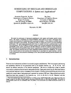
Figure 1: Vertex insertion (a), bisection of a right triangle (b), and corresponding conforming modification (c). M −1 = (T2 , T1 ). A modification M =(T1 , T2 ) is a refinement modification if #T2 > #T1 . Conversely, M is a coarsening modification if #T2 < #T1 . We also denote the two meshes forming a modification M with M − and M + , according to the intuition that M − has fewer cells than M + . A Multi-resolution Triangle mesh, or Multi-Triangulation (MT) consists of a mesh T0 , called the base mesh, of a set of conforming refinement modifications {M1 , M2 , . . . Mh }, and of a partial order defined among the modifications. Each triangle t involved in a modification must either appear in T0 , or be created by one modification of the set. The partial order is defined as the transitive closure of the following dependency relation: a modification Mj depends on a modification Mi if Mj removes some triangle inserted by Mi . Intuitively, dependency means that Mj can be applied only if Mi has been applied before. An MT provides a compact way of encoding all conforming meshes that can be obtained by applying some of the given modifications to the base mesh. A subset S of {M1 , . . . Mh } is called closed with respect to the partial order if, for each modification Mi ∈ S, all modifications Mj , such that Mi depends on Mj , are also in S. The modifications in a closed subset S can be applied to the base mesh T0 in any total order extending the partial one, and always give the same mesh TS , that we call an extracted mesh. In particular, the extracted mesh obtained by applying all modifications {M1 , . . . Mh } to the base mesh is called the reference mesh, and it is denoted with T∞ . Any triangle mesh formed by combining the triangles of an MT can be obtained from some closed set [17]. A closed set S containing more updates in some areas and fewer updates elsewhere produces a mesh having a resolution variable through the domain.
3.1 Vertex-Based MTs and Hierarchies of Right Triangles Specific multi-resolution models are defined by considering specific modification operators. Two relevant examples of modification operators for triangle meshes are vertex insertion, its inverse vertex removal, and bisection of right triangles (see Figures 1(a) and (b)). Vertex insertion deletes a connected set of triangles in the neighborhood of the vertex v to be inserted. The choice of such triangles depends on the specific algorithm used: a typical example is vertex insertion in a Delaunay triangulation. The hole left by the removed triangles is filled with new triangles incident at v. Vertex removal is the inverse modification of a vertex insertion. The removal of a vertex v deletes the triangles incident at v, thus leaving a hole bounded by a star-shaped polygon. New triangles are created which fill the hole by triangulating the polygon. Both vertex insertion and removal are conforming modifications since they do not change the edges on the boundary of the modification.
Right-triangle bisection operates on a triangle mesh consisting of right triangles with vertices at a regular grid. It splits a triangle into two triangles at the mid-point of its longest edge. It is not a conforming modification. In order to produce conforming meshes, we cluster two right-triangle bisections occurring at a pair of right isosceles triangles t1 and t2 , sharing their longest edge, into a conforming modification that replaces t1 and t2 with four right triangles (see Figure 1 (c)). A vertex-based MT is an irregular MT in which every modification Mi is a vertex insertion. T0 is an arbitrary triangle mesh covering the domain of the height field. A vertex-based MT can be constructed by top-down refinement through iterative vertex insertion (based, for instance, on on-line algorithms for Delaunay triangulation), or by bottom-up coarsening through iterative vertex removal starting from the reference mesh T∞ [4]. The vertex to be inserted (removed) can be chosen either randomly, or according to an errordriven greedy strategy, which tends to maximize the error decrease at each vertex insertion (to minimize the error increase at each vertex removal). In coarsening, a maximal set of independent vertices, affecting disjoint sets of triangles, are often removed simultaneously. A Hierarchy of Right Triangles (HRT) is an MT built from points on a regular grid of n = (2k + 1) × (2k + 1) points, where k is a positive integer. The base mesh is obtained by splitting the square domain through one of its diagonals. All modifications are bisections of right triangles. An HRT is usually built top-down through the iterative application of the triangle bisection rule.
3.2 Level-Of-Detail (LOD) queries on a multiresolution terrain model A multi-resolution mesh can be used as a tool for on-line generation of TINs describing a terrain, in which the Level Of Detail (LOD) is not uniform, and satisfies some userdefined criteria. Selective refinement is the operation of extracting a mesh in which some terrain portions are refined up to some extent defined by the user. In an applicationindependent formulation, the parameters of a selective refinement query are two Boolean functions defined on the triangles of a multi-resolution mesh: a focus condition, which selects the portion of the terrain relevant to the query, and a LOD threshold, which defines the desired resolution. The focus condition is true on a triangle t if and only if t is considered to be relevant. The LOD threshold is true on t if and only if the level of detail of t is considered sufficient. The LOD threshold is applied just to the triangles selected by the focus condition. A selective refinement query is answered by finding a closed subset of modifications such that, in the corresponding extracted TIN, all triangles that are selected by the focus condition satisfy the LOD threshold. Algorithms for selective refinement on an MT are described in [4]. Focus conditions can be defined based on the spatial location of a triangle, on its elevation, slope, or attributes (soil type, land use, etc.). For instance, a focus condition that selects just triangles interfering with an entity (point, line, region) in the domain can be used to evaluate local terrain characteristics. For computing a contour line, for instrance, we select just triangles containing a given elevation. LOD thresholds can be defined based on the spatial location of a triangle, on its geometric properties (e.g., size,
shape), or on its accuracy-related attributes (e.g., error in approximating elevation or slope). Usually, a LOD threshold is defined based on the error, and imposes an upper bound on the elevation error allowed for a given triangle, where the bound can be either a constant, or a function. In this paper, we consider selective refinement queries with an error-based LOD threshold. For this purpose, we define the approximation error of a triangle t, based on the points of the data set which are inside t. The approximation error associated with t is, thus, the maximum vertical distance of a point whose projection is inside t from the plane defined by the vertices of t and by their elevation values, where the maximum is taken over all points whose projection is inside t.
4. DATA STRUCTURES In this section, we describe two data structures to encode a vertex-based MT, and an HRT, respectively. In evaluating space requirements, we assume to store vertex coordinates, elevations, and approximation errors in two bytes. Pointers and indices are stored in four bytes. We denote with n the number of vertices in the reference mesh T∞ , i.e., the total number of vertices in an MT. The number of triangles in T∞ is about 2n. Assuming the base mesh T0 to be very small, the number of modifications is roughly equal to n.
4.1 Encoding a Vertex-based MT A data structure for a vertex-based MT must encode the partial order, and the modifications. The partial order is maintained according to a technique proposed by Klein and Gumhold [12], which encodes each dependency link only once. The cost of storing the dependency relation has been evaluated to be equal to 4(a+n) bytes, where a is the number of dependency links. Experimentally, we have found that, in a vertex-based MT, a ' 3n. Thus, the cost of storing the dependencies becomes equal to 16n bytes. Given a modification M in a vertex-based MT, we denote with vM the vertex inserted by M , and with πM the common polygonal boundary (chain of edges) of M − and M + . Modifications and vertices are re-numbered in such a way that a node M and its corresponding vertex vM have the same label. To encode a modification M , we store the coordinates of vertex vM , the value of the elevation at vM , error information, plus information needed to perform M and its inverse M −1 on the current mesh TS . The first two items require 6n bytes in total. The last two items are described in the following. In performing M , the difficult task is recognizing the triangles of M − (to be deleted) in TS . The triangles of M + (to be created) are easily obtained by joining the edges of πM to vM . In performing M −1 , the triangles of M + (to be deleted) are those incident at vM . The difficult task here is reconstructing the triangles of M − which form a triangulation of πM . The technique we use for encoding the triangulation of πM is based on an approach proposed by Taubin et al. [20] in the context of progressive mesh compression. Other techniques are analyzed and compared in [1]. For each modification M , we store one edge eM of polygon πM , that we call the anchor edge, plus a bit stream encoding a sequence of the triangles of the triangulation M − of πM sorted according to a depth-first traversal of M − . A compact encoding of eM requires 10 bits for each modification. The bit stream contains two bits for each triangle of
0
00
000 001
Terrain
points
triangles in T∞
Mount Marcy
16641
32768
Devil Peak
16641
32768
1
10
01
010 011
100
101
11
110 111
Figure 2: The trees describing an HRT and the location codes corresponding to its triangles.
M − . Summing up over modifications, we have 2t bits in all streams, where t is the number of triangles in the MT which do not belong to the reference mesh. It has been experimentally found that t ' 4n. It follows that 18n bits, i.e., 3n bytes are sufficient to describe the anchor edges and the bit streams for all modifications. Error information can be stored for each triangle of M − by using an array sorted according to the order of its triangles in the bit stream. The cost is 2t bytes, i.e., about 8n bytes. Alternatively, a single error can be stored for each modification M , computed as maximum of the errors associated with the triangles in M − , with a cost of 2n bytes. Summing up the space requirements for the partial order and the modifications, we have 33n bytes if we store errors associated with triangles, and 27n bytes if we store errors associated with modifications. A data structure for encoding the reference mesh, storing vertex coordinates, triangles in an indexed format, and adjacency links between pairs of triangles sharing an edge, would require 54n bytes. Thus, a vertex-based MT achieves a compression factor of 0.6 (with errors on triangles), or 0.5 (with errors on modifications) with respect to the mesh at full resolution.
4.2 Encoding a Hierarchy of Right Triangles In an HRT, the modifications, the triangles, and the dependency relation are implicitly defined on the basis of fixed patterns. The data structure consists of a table containing the elevation values at the n data points, and of two almost full binary trees, containing the errors associated with the triangles, encoded as arrays. The two trees describe the complete subdivision of the square defining the domain boundary, except for the last level which corresponds to triangles of the reference mesh (and, thus, with a null error). We use a location code [18] for each triangle to index the elevation table and to find the neighbors of a triangle. The location code of a triangle t is a variable-length bit stream encoding the path from the root of the tree to t and by concatenating one bit for each traversed arc. The bit is equal to 0 (1) if the arc leads to a left (right) child (see Figure 2). We define the left and the right child of a triangle t by considering the splitting edge directed towards the right angle vertex of t. The length of the location code corresponds to the level of t in the tree, i.e., to its size. The location codes of the parent and of the children of a triangle t are obtained from that of t by removing and concatenating a bit, respectively. The vertices of a triangle t are also computed from the location code of t.
MT VI VR IVR HRT VI VR IVR HRT
triangles in MT (%T∞ ) 81655 (2.49) 99045 (3.02) 94093 (2.87) 65534 (2) 83018 (2.53) 100813 (3.07) 94729 (2.89) 65534 (2)
size (bytes) 391611 454427 413945 98814 393178 445765 413347 98814
Table 1: Characteristics of the MTs built for the two reference data sets. The conforming modifications associated with triangle bisections and the dependency relation are implicitly encoded by the two trees describing the nesting structure of the triangle in the decomposition. Conforming modifications are computed when extracting a mesh by efficient neighbor finding techniques which have a constant worst-case behavior, being based on arithmetic manipulation of the location codes [8, 13]. The number of triangles in the trees is about 2n. This yields to a storage cost of 4n bytes for the array containing the error values plus 2n bytes for the elevation table, leading to a total cost of 6n bytes. Thus, the storage cost of an HRT is about 1/5 of the cost of a vertex-based MT.
5. RESULTS AND COMPARISONS We present experiments on two terrain data sets: Mount Marcy, and Devil Peak (data courtesy of U.S. Geological Survey). We have considered a regular grid of 129 × 129 points. Vertex-based MTs have been constructed through vertex insertion (VI), removal of a single vertex (VR), and removal of sets of independent vertices (IVR) in a Delaunay triangle mesh. All MTs have two triangles in the base mesh T0 , and 32768 triangles in the reference mesh T∞ . Table 1 also reports the total number of triangles in the MTs (including those of T∞ ), and the size of the corresponding data structures (in bytes). The HRT has the smallest number of triangles, which is independent of the specific data set. The most compact data structure, among the three vertex-based MTs, is that for VI, the least compact is the one for VR. We have measured the number of extracted triangles in the different queries. This parameter is directly related to extraction times as well as to the time necessary for further, application-dependent, processing to be performed on the extracted mesh (e.g., rendering). We have considered the extraction of a TIN at a uniform LOD over the domain, and of TINs which have a high resolution just in a rectangular window in their domain, or at a given elevation value. They are the variable-resolution formulation of a windowing query, and an iso-line query, respectively. This is achieved by performing selective refinement with a constant LOD threshold and a focus condition defined to be true on all triangles (uniform case), or just on triangles whose projections in the x-y plane interfere with the given window, or on triangles interfering with a plane at the specified elevation value (for the other queries). Figures 2, 3, and 4 report the results. The best MT corresponds to the curve closest to the horizontal axis. In the uniform case, the vertex-based MT built through vertex insertion (VI) shows the best performances. The other three MTs show no relevant differences. The reason for this is that the VI construction follows a
completely error-guided strategy. Techniques VR and IVR are also error-driven, but the error in removing a vertex is estimated through heuristics (since an exact computation would be too expensive). In the HRT the modifications are constrained by a fixed splitting rule. For the window queries, the HRT is the best, the VR vertex-based MT is the worst, while the other two vertexbased MTs are roughly equivalent. This because the modifications in an HRT are smaller, thus it is more effective in refining the representation only locally. In vertex-based MTs, the average number of triangles in M − is equal to 4, the maximum is equal to 10, while, in an HRT, this number is always equal to 2.
6.
CONCLUDING REMARKS
We have compared multi-resolution models for representing a terrain, based on a regular and on an irregular triangle mesh. A vertex-based MT can deal with both irregularly and regularly-distributed data points, while an HRT is specific for regular data sets. The data structure for an HRT is very compact, but that for a vertex-based MT is still considerably more economical than encoding the mesh at full resolution. Experiments show that an HRT provides a good compression ratio for selective refinement queries at variable resolution with a narrow focus, while a vertex-based MT is more effective for queries at a uniform LOD. An important common feature is that in both cases the connectivity of the extracted mesh is generated at no extra cost. This is fundamental for applications involving geometric navigation and computations on the mesh (e.g., contour line extraction, drainage network computation, path planning, etc.).
[7]
[8]
[9]
[10]
[11]
[12]
[13]
[14]
Acknowledgement
[15]
This work has been supported by the project funded by the Italian Ministry of University, Education and Research (MIUR) on Representation and Processing of Spatial Data in Geographic Information Systems.
[16]
7.
REFERENCES
[1] E. Danovaro, L. De Floriani, P. Magillo, and E. Puppo. Compressing multiresolution triangle meshes. In C. Jensen, M. Schneider, B. Seeger, and V. Tsotras, editors, Lecture Notes in Computer Science, volume 2121, Springer-Verlag, pages 345–364. 2001. [2] M. de Berg and K. Dobrindt. On levels of detail in terrains. In Proceedings 11th ACM Symposium on Computational Geometry, Vancouver (Canada), ACM Press, pages C26–C27, 1995. [3] L. De Floriani. A pyramidal data structure for triangle-based surface description. IEEE Computer Graphics and Applications, 8(2):67–78, 1989. [4] L. De Floriani and P. Magillo. Multiresolution mesh representation: Models and data structures. In M.Floater, A.Iske, and E.Qwak, editors, Tutorials on Multiresolution in Geometric Modelling, pages 363–418. Springer-Verlag, 2002. [5] L. De Floriani, P. Magillo, and E. Puppo. VARIANT: A system for terrain modeling at variable resolution. Geoinformatica, 4(3):287–315, 2000. [6] L. De Floriani and E. Puppo. Hierarchical triangulation for multiresolution surface description.
[17] [18]
[19]
[20]
[21]
[22]
ACM Transactions on Computers, 14(4):363–411, 1995. M. Duchaineau, M. Wolinsky, D. Sigeti, M. Miller, C. Aldrich, and M. Mineed-Weinstein. ROAMing terrain: Real-time optimally adapting meshes. In R. Yagel and H. Hagen, editors, Proceedings IEEE Visualization’97, pages 81–88, 1997. W. Evans, D. Kirkpatrick, and G. Townsend. Right-triangulated irregular networks. Algorithmica, 30(2):264–286, 2001. D. Gomez and A. Guzman. Digital model for three-dimensional surface representation. Geo-Processing, 1:53–70, 1979. H. Hoppe. Progressive meshes. In Computer Graphics (SIGGRAPH ’96 Proceedings), ACM Press, pages 99–108. 1996. H. Hoppe. Smooth view-dependent level-of-detail control and its application to terrain rendering. In Proceedings IEEE Visualization’98, IEEE Computer Society, pages 35–42, 1998. R. Klein and S. Gumhold. Data compression of multiresolution surfaces. In Visualization in Scientific Computing ’98, Springer-Verlag, pages 13–24. 1998. M. Lee, L. De Floriani, M., and H. Samet. Constant-time neighbor finding in hierarchical meshes. In Proceedings International Conference on Shape Modeling, Genova, May 2001, pages 286–295, 2001. P. Lindstrom, D. Koller, W. Ribarsky, L. Hodges, N. Faust, and G. Turner. Real-time, continuous level of detail rendering of height fields. In ACM Computer Graphics (SIGGRAPH ’96 Proceedings), ACM Press, pages 109–118, 1996. A. Maheshwari, P. Morin, and J.-R. Sack. Progressive TINs: Algorithms and applications. In Proceedings 5th ACM Workshop on Advances in Geographic Information Systems, ACM Press, 1997. R. Pajarola. Large scale terrain visualization using the restricted quadtree triangulation. In D. Ebert, H. Hagen, and H. Rushmeier, editors, Proceedings IEEE Visualization’98, IEEE Computer Society, pages 19–26, 1998. E. Puppo. Variable resolution triangulations. Computational Geometry, 11(3-4):219–238, 1998. H. Samet. Applications of Spatial Data Structures: Computer Graphics, Image Progessing, and GIS. Addison Wesley, Reading, MA, 1990. R. Sivan and H. Samet. Algorithms for constructing quadtree surface maps. In Proceedings 5th International Symposium on Spatial Data Handling, pages 361–370, 1992. G. Taubin, A. Gu´eziec, W. Horn, and F. Lazarus. Progressive forest split compression. In Computer Graphics (SIGGRAPH ’98 Proceedings), pages 123–132. ACM Press, 1998. B. Von Herzen and A. Barr. Accurate triangulations of deformed, intersecting surfaces. Computer Graphics (SIGGRAPH 87 Proceedings), 21(4):103–110, 1987. J. Xia, J. El-Sana, and A. Varshney. Adaptive real-time level-of-detail-based rendering for polygonal models. IEEE Transactions on Visualization and Computer Graphics, 3(2):171–183, 1997.
33000
33000
30000
30000
27000
27000
24000
24000
21000
21000
18000
18000
15000
15000
12000
12000
9000
9000
6000
6000
3000
3000
0.00
0.00 0
error value
50%
0
Mount Marcy
error value
50%
Devil Peak
Table 2: Extracted triangles with an uniform error bound. The bound ranges from 0 to half of the elevation range of the terrain. The line styles are as follows: plain = HRT, dashed = VI, plain with circles = IVR, dashed with circles = VR. 7000
7000
6000
6000
5000
5000
4000
4000
3000
3000
2000
2000
1000
1000
0.00
0.00 1%
box edge
15%
1%
Mount Marcy
box edge
15%
Devil Peak
Table 3: Extracted triangles with zero error bound, focused in a window. The length of the window edge ranges from 1% to 15% of the edge of the domain of the height field. The line styles are as in Table 2.
12000
15000
11000
13500
10000
12000
9000 10500
8000 7000
9000
6000
7500
5000
6000
4000
4500
3000 3000
2000
1500
1000 0.00
0.00 0
height value
Mount Marcy
100%
0
height value
100%
Devil Peak
Table 4: Extracted triangles with zero error bound, focused on an elevation value. The elevation ranges from the minimum to the maximum over the the terrain. The line styles are as in Table 2.