High performance CPU/GPU multiresolution ... - Semantic Scholar

Parallel Computing: Accelerating Computational Science and Engineering (CSE) M. Bader et al. (Eds.) IOS Press, 2014 © 2014 The authors and IOS Press. All rights reserved. doi:10.3233/978-1-61499-381-0-481

481

High performance CPU/GPU multiresolution Poisson solver Wim M. VAN REES, Diego ROSSINELLI, Panagiotis HADJIDOUKAS and Petros KOUMOUTSAKOS 1 Chair of Computational Science, ETH Z¨urich, Switzerland Abstract. We present a multipole-based N-body solver for 3D multiresolution, block-structured grids. The solver is designed for a single heterogeneous CPU/GPU compute node, and evaluates the multipole expansions on the CPU while offloading the compute-heavy particle-particle interactions to the GPU. The regular structure of the destination points is exploited for data parallelism on the CPU, to reduce data transfer to the GPU and to minimize memory accesses during evaluation of the direct and indirect interactions. The algorithmic improvements together with HPC techniques lead to 81% and 96% of the upper bound performance for the CPU and GPU parts, respectively. Keywords. tree-code, multipole method, GPU, vortex method, multiresolution

Introduction Multipole methods are used to decrease the computational cost of the N-body problem encountered in many particle-based simulations with applications such as astrophysics and fluid mechanics. Much effort is devoted to optimizing the performance of multipolebased N-body solvers for arbitrarily spaced source and destination particles, both for massively parallel distributed memory architectures [1] and for GPUs and GPU clusters [2]. In fluid mechanics, the N-body problem lies at the heart of traditional vortex methods [3]. The kinematic relationship between vorticity and the streamfunction leads to an N-body potential problem that needs to be solved at every timestep to recover the streamfunction from the vorticity. In the current work we consider remeshed vortex methods [4], which combine particle-based advection with regular grid-based data representations. The regular grid is commonly exploited for FFT-based elliptic solvers [5]. However, the straightforward use of FFT-based solvers is hindered in a multiresolution setting, where the grid spacing changes according to the local spatial scales in the flow. For multiresolution remeshed vortex methods, multipole methods offer a number of computational advantages. First, they can handle arbitrarily spaced source and destination points. Second, their computational cost scales separately with the number of source and destination points. This is relevant here since in general the vorticity field has a compact support, whereas the streamfunction needs to be evaluated globally. Third, they al1 Corresponding

Author: [email protected]

482

W.M. Van Rees et al. / High Performance CPU/GPU Multiresolution Poisson Solver

low for a natural treatment of free-space boundary conditions. And fourth, the granularity of the computational work is relatively fine as every destination point can be evaluated independently, rendering the use of GPU-based acceleration techniques particularly attractive. In this work we present a multipole-based N-body solver to compute the streamfunction from the vorticity field on a multiresolution grid. As opposed to existing algorithms, we designed our solver to exploit the regular structure of the destination points. We outline the algorithm, present details of our optimizations and show performance results of the heterogeneous CPU/GPU implementation on a single Cray XK7 compute node. 1. Governing equations The remeshed vortex method solves the Navier-Stokes equations in the velocity (u)vorticity (ω = ∇ × u) formulation. At every timestep, the velocity field needs to be computed from the vorticity field. Using the incompressibility of the velocity field (∇ · u = 0), one can derive a Poisson equation for the solenoidal vector streamfunction Ψ: ∇2 Ψ = −ω,

(1)

from which the velocity follows as u = ∇ × Ψ. Throughout this work we consider one component of the above Poisson equation, and employ free-space boundary conditions to simulate an unbounded flow. The solution to equation (1) can be written as a convolution between Green’s function for the Laplace equation and the right-hand side: Ψ(x) = −

!

G(x − x′ )ω(x′ ) dx′ ,

(2)

where, in three dimensions, G(x) = −

1 . 4π|x|

(3)

Here we will briefly recapitulate the multipole method, based on [6] and following the discussion in [7]. In the discrete case, for N source points located inside a sphere with radius a, and the ith source point having polar coordinates (ri′ , θi′ , φi′ ) and weight ωi , we have at polar location x = (r, θ , φ ): N

ω ωi 1 N " i "= # , ∑ ′ ′ " " 2 4πr i=0 1 + (ri /r) − 2(ri′ /r) cos γi i=0 4π x − xi

ψ(x) = ∑

(4)

where γi is the angle between the vectors x and x′i . If for each source point we have (ri′ /r) < 1, we can substitute the definition of Legendre polynomials Pn (x) as Taylor series, and use the addition theory for spherical harmonics Ynm (θ , φ ) to find 1 ψ(x) = 4π

∞

n

∑ ∑

n=0 m=−n

$

N

∑

i=0

%

n ωi r′ i Ynm (θi′ , φi′ )

Ynm (θ , φ ) 1 ≡ n+1 r 4π

∞

n

∑ ∑

n=0 m=−n

Cnm

Ynm (θ , φ ) . (5) rn+1


483

In this expression, the multipole coefficients Cnm can be precomputed for each collection of sources, and used in the evaluation of equation (5) for every destination point. If the infinite sum over n is truncated to a finite number of terms p + 1, the following error norm holds: " " " " & a ' p+1 N m 1 p n " m Yn (θ , φ ) " C . (6) "ψ(x) − " ≤ ∑ |ωi | (r − a)−1 ∑ ∑ n n+1 " " i=1 4π n=0 m=−n r r

Evaluation of the direct interactions requires a discretization of equation (2), with the Green’s function given in equation (3). The singular nature of this integral reduces the accuracy of the scheme close to the singularity. Furthermore, it requires special treatment of the singularity itself, i.e. the case x = x′ , which introduces an instruction irregularity in the code. For these reasons we choose to replace the original Green’s function with a smoother function, as derived in [8]: Gε (r) = −

1 r2 + 23 ε 2 , 4π (r2 + ε 2 ) 32

(7)

where ε is a smoothing parameter. In our simulations, we set ε = h, where h is the smallest grid spacing in the domain. This formulation removes the singularity and associated instruction irregularity, and improves the accuracy of the results. 2. Computational setting The multipole solver described herein is part of a 3D incompressible fluid mechanics solver under development. The solver is built on MRAG, a wavelet-based, multiresolution block-structured framework to solve partial differential equations [9], and is based on the remeshed vortex method [10]. In the remeshed vortex method each timestep requires three executions of the multipole algorithm, once for each of the three components of the streamfunction. Future applications of the solver include the simulation and optimization of self-propelled swimmers [11,12]. In MRAG, the computational grid consists of blocks with a fixed number of gridpoints in each direction (here 16). The computational blocks are non-overlapping leaves of a hierarchical tree structure that represents the computational grid, so that each block can exist at a different spatial resolution. Blocks can be refined (split into new blocks) or compressed (merged with neighboring blocks) based on the magnitude of the detail coefficients in the forward wavelet transform of relevant quantities with respect to userspecified thresholds. Operations across all blocks are parallelized on a multicore node with task-based parallelism, based on the work-stealing principle as implemented in the Intel Threading Building Blocks (TBB) library [13]. More details on MRAG and its parallel implementation on multicore CPUs are given in [9,14]. 3. Algorithm The algorithm used here is based on a Barnes-Hut tree code [6] and adapted for the current computational setting.

484


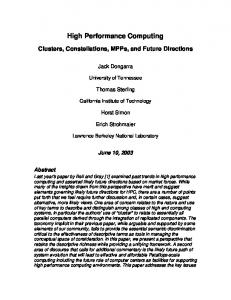
We filter all grid points to extract those with non-zero vorticity values, creating an array of source points spanning only the support of the vorticity field. These source points are hierarchically decomposed into an oct-tree structure, guided by a parameter controlling the maximum number of source points per leaf (smax , here set to 2048). For each leaf the multipole expansion coefficients Cnm are calculated according to equation (5). At parent nodes the expansions of the children are combined and translated to the parent centers [7]. All expansions are stored in an array. We group a set of destination points into a brick (here 8 grid points in each direction) to increase the amount of work per task. All points in a destination brick are subjected to the same logical interaction pattern. For each destination brick, therefore, we create two logical plans containing the lists of all direct and all indirect interactions, respectively. Separating the creation of the plan from the actual interaction evaluations enables offloading of all direct interactions to an accelerator such as the GPU. The logical plans are based on a user-specified opening parameter θ . Specifically, for each destination brick, we traverse the source tree downwards. Starting at the root node, we compare the node radius a (the radius of the smallest sphere containing its sources) with the smallest distance r between the node center and the points inside the destination brick. If a/r < θ , we will perform a multipole evaluation according to equation (5) between the tree node and all points in the destination brick. If a/r ≥ θ , we traverse one level down the tree and repeat the process for all the node’s children. If we reach a leaf, we perform direct evaluations according to equation (4) between all points in the source node and all points in the destination brick. In this way, if θ = 0 we perform the O(N 2 ) problem whereas for 0 < θ < 1 we have a converging multipole approximation with truncation error bound by equation (6), as a function of the order of the multipole expansion p and the opening parameter θ . The logical plan for the direct evaluations of a destination brick consists of a vector of pairs, where each pair encodes the start and the end index of a range in the source point arrays (see figure 1). For the indirect evaluations, the logical plan consists of a vector of tuples, where each tuple contains the 3D center of the expansions and the index of the expansion in the expansions array. Finally, we evaluate the logical plans for each destination brick and sum the results to obtain the streamfunction field.

4. Implementation The algorithm is implemented in C++11 and is parallelized using OpenMP tasks and the Threading Building Blocks (TBB) library. The order of the multipole expansion p, is a compile-time constant that is fixed at p = 6 in this work. In this section we will briefly discuss the implementation of the key parts of the algorithm. Source points The source points are converted from an Array-of-Structures (AoS) to a Structure-of-Arrays (SoA) format to enable vectorization over the source particles in the later stages of the solver. To increase spatial locality, we sort the particles in Morton order with the OpenMP-based GNU libstdc++ parallel sort.


485

Figure 1. Logical plan for the direct interactions. The source point arrays (top, green) are the set of grid points with non-zero vorticity, converted to a Structure of Arrays (SoA). For each structured, fixed-size destination brick the plan defines a list of pairs representing the start and end indices (inclusive) of the source points to interact with. For simplicity, destination bricks in this sketch are represented as 2D blocks of 4 × 4 grid points.

Tree construction and logical plan The oct-tree containing all source particles is recursively constructed using OpenMP tasks. We first perform a top-down pass to identify and create the nodes on each level, and then perform a bottom-up pass to compute the multipole coefficients Cnm according to equation (5). After the tree construction, the logical plan for the evaluation phase is created using TBB parallel tasks across the destination bricks. Legendre polynomials Pnm The associated Legendre polynomials Pnm (cos θ ) are evaluated for 0 ≤ n ≤ p, 0 ≤ m ≤ n through the recursive equations: P00 = 1, Pn0 =

P10 = cos(θ ),

P11 = sin(θ )

(2n − 1) (n − 1) 0 0 cos(θ )Pn−1 Pn−2 − n n

m−1 m Pnm = (2n − 1) sin(θ )Pn−1 + Pn−2

m−1 Pnm = (2n − 1) sin(θ )Pn−1

2≤n≤ p 2 ≤ n ≤ p,

1 ≤ m ≤ n−2

2 ≤ n ≤ p,

n−1 ≤ m ≤ n

We store the polynomials in a linear data structure of size (p+1)(p+2)/2. All recursions are templatized over n, and for each n in turn over m, so that all instruction irregularity is resolved at compile-time and array access indices can be precomputed. Furthermore, the associated Legendre polynomials are vectorized with SSE instructions so that the values of Pnm can be computed for four different arguments in one set of operations. Spherical harmonics Ynm

The spherical harmonics Ynm (θ , φ ) are defined as: ( (n − |m|)! |m| m Yn (θ , φ ) = Pn (cos θ ) (cos(mφ ) + i sin(mφ )) , (n + |m|)!

for 0 ≤ n ≤ p and −m ≤ n ≤ m. To reduce the number of costly trigonometric evaluations, we compute the sine and cosine factors recursively using the identity:

486


sin(mφ ) = sin(φ ) cos((m − 1)φ ) + cos(φ ) sin((m − 1)φ ),

cos(mφ ) = cos(φ ) cos((m − 1)φ ) − sin(φ ) sin((m − 1)φ ). Finally we note that the prefactor in the definition of the spherical harmonics, for m > 0, can be rewritten as: (n − m)! 1 = . (n + m)! (n + m)(n + m − 1)(n + m − 2) . . . (n − m + 1) This formulation reduces the number of floating point evaluations and is precomputed for all n ≤ p and m ≤ n at compile-time. The spherical harmonics are stored into two arrays, each of size p(p + 1)/2, for the real and complex part, respectively. Again we vectorize the computation using SSE so that we can compute the set of all harmonics for four different arguments (θ , φ ) in parallel. Multipole coefficients Cnm When creating the multipole coefficients Cnm from a set of source particles, we use SSE instructions to process four source points in parallel. Again template recursion allows for unrolled instructions over the n and m indices. The values Cnm are stored in three arrays: two of size p(p + 1)/2 for the real and imaginary part of Cnm , m > 0, and one more of size (p + 1) for the m = 0 values. Based on the multipole coefficients for a leaf node of our source tree, we can use translation equations to find the coefficients at parent nodes [7]. In this translation computation we use a precomputed look-up table for those prefactors known at compile-time. CPU-only evaluation When evaluating both indirect and direct interactions on the CPU, we rely on three levels of TBB-based parallel operators to exploit the multicore architecture. The first level of parallelism covers all the bricks, the second covers the direct and the indirect interactions, and the third covers the interactions themselves. At the finest level of parallelism we therefore evaluate a (sub)set of interactions (direct or indirect) for all the destination points inside a brick. The direct evaluation kernel on the CPU is vectorized with AVX instructions. Since our bricks consist of 8 grid points per dimension, this allows us to evaluate all the grid points along the x-direction in parallel. Based on equation (7), we have 15 floating-point operations and 1 reciprocal square root per particle-particle interaction. We implement the reciprocal square root with the AVX native approximation and a further NewtonRaphson iteration, leading to a total cost of 21 floating point operations. Out of these 21 operations, 4 are Fused Multiply-Add (FMA) operations. The indirect evaluation kernel on the CPU is currently vectorized with SSE instructions over the destination points along the x-direction. These instructions are unrolled at compile-time with templates. Here we count the number of instructions directly from the assembly code, which gives 46 floating point operations per particle-multipole interaction (for p = 6), out of which 11 are FMA. Hybrid CPU/GPU evaluation In case we use the GPU to evaluate the direct interactions, we send the source data to the GPU right after creating the SoA source arrays, so that the transfer overlaps with the next steps on the CPU: computing the multipole coefficients and creating the logical evaluation plans. After the plans and the tree are created, we send the logical plan for the direct evaluations to the GPU and start the evalua-


487

CPU create source particles

create tree & expansions

send sources

GPU

receive source particles

create logical plan

evaluate indirect interactions

send plan receive logical plan

accumulate results send results

evaluate direct interactions

Figure 2. Hybrid CPU/GPU workflow, showing the steps on the CPU (red) and GPU (blue) for one streamfunction evaluation.

tion asynchronously, so that it is executed in parallel with the evaluation of the indirect interactions on the CPU. Finally, we transfer back the results from the GPU (figure 2). The GPU implementation maps all direct interactions for a single destination brick on one streaming multiprocessor (SM), so that each CUDA block is a 3D array with 8 threads in each direction. If the number of bricks exceeds the maximum CUDA grid size, we perform multiple passes. We use the shared memory on an SM to load up to 64 source point locations and weights in parallel, and subsequently each CUDA thread in the SM evaluates those source points for its own destination point. The interaction kernel performs 15 FLOPs (including 3 FMA) and 1 reciprocal square root with a cost equivalent to 6 FLOPs [15]. The amount of direct interactions to be computed generally varies between the bricks, which could lead to load-imbalance. However, we found that the hardware scheduler on the GPU is effective in distributing the work among the available SMs and we did not observe significant load-imbalance problems. 5. Results We run our performance tests on a single 16-core AMD Interlagos 6272 compute node, with a NVIDIA Tesla K20X GPU, as available on the Cray XK7 system “T¨odi” at the Swiss Supercomputing Center (CSCS). The peak performance of all 8 FPUs of this compute node is 268.8 GFLOP/s, and the listed peak performance of the K20X is 3.95 TFLOP/s. Both the CPU and GPU support FMA instructions, so the upper performance bounds of our kernels are adjusted according to their FMA/non-FMA ratios. The code is compiled with version 4.7 of the GNU C++ compiler and version 4.1.0 of TBB. We consider two test cases: the first is an artificial constructed test problem while the second considers a relevant flow problem. 5.1. Test problem We consider a test problem introduced in [16], consisting of a vortex ring with radius R, its streamfunction defined as: . / ⎧ * )# ⎨c exp − c2 if |t| < 1 (r − R)2 + z2 1 1 − t2 eθ , where f (t) = . Ψ(r, z) = f ⎩ R 0.0 else

The vorticity is derived from the streamfunction as ω = ∇ × (∇ × Ψ). We place a ring at (0.25, 0.25, 0.25) and at (0.75, 0.75, 0.75) in a unit cube domain with origin (0, 0, 0).

488


hybrid CPU/GPU

CPU only

4.8E-03 8.4E-03 1.3E-02

1.3E-02

7.8E-03 7.8E-03

7.1E-02

6.6E+00

6.8E-01

8.5E-02 8.6E-03

4.2E-02 8.6E-03 4.2E-02

evaluation other

evaluation other

create logical plan create tree & expansions source arrays SoA transform sort source arrays

create logical plan create tree & expansions source arrays SoA transform sort source arrays transfer sources & plan to GPU transfer results from GPU

Figure 3. Time distribution (in seconds) of the presented algorithm with θ = 0.5, CPU-only (left) and hybrid CPU/GPU (right)

CPU only

hybrid CPU/GPU

1.0E+03

1.0E+03

indirect interactions direct interactions total evaluation

indirect interactions (CPU) direct interactions (GPU) total evaluation

1.0E+02

Wall-clock time (s)

Wall-clock time (s)

1.0E+02

1.0E+01

1.0E+00

1.0E-01

1.0E+01

1.0E+00

1.0E-01

1.0E-02

1.0E-02 0

0.1

0.2

0.3

0.4

0.5

θ

0.6

0.7

0.8

0.9

1.0

0

0.1

0.2

0.3

0.4

0.5

0.6

0.7

0.8

0.9

1.0

θ

Figure 4. Time spend in computing direct and indirect interactions as a function of θ , CPU-only (left) and hybrid CPU/GPU (right)

For each ring, we set R = 0.125, c1 = 227 and c2 = 20. We rotate one of the rings by π/2 so that the axes of the rings are not aligned. The effective resolution of the grid is 2563 , with compression and refinement thresholds of 10−4 and 10−2 , respectively, resulting in 3.6 × 106 destination points. We consider the y-component of the streamfunction, for which we have 8.7 × 105 source particles. In figure 3 we show the time distribution of the CPU implementation (left) and CPU/GPU implementation (right) for the case of θ = 0.5. The evaluation phase, which covers both the direct and indirect interactions, takes most of the time for both cases. The remaining time is spent mostly in sorting the source particles, after that it is about equally spent in the remaining parts of the algorithm. Since the evaluation phase takes most of the time, we focus our analysis there. Strong parallel scaling of the evaluation step on the CPU reaches 96.7% on 8 cores, in which case all FPUs are active. Doubling the number of cores to 16 brings only very small improvements for the evaluation phase, although other parts of the solver, notably the creation of the logical plan, benefit from these additional cores. Details about the evaluation phase are shown in figure 4. For the parallel parts of the code, we accumulate the timings measured for each brick and divide this number by the total number of threads (16), to obtain a measure of the wall-clock time spent in each phase of the evaluation. We plot the timings against different values of θ . The time spent


489

Figure 5. Performance measurements from simulations of the flow past a sphere, with effective resolution of 5123 (blue) and 10243 (red).

per interaction evaluation remains approximately constant for both the direct (CPU and GPU) and the indirect evaluations. For the CPU-only execution, across the entire range of θ values, we spend at least one order of magnitude more time for the direct interactions than for the indirect interactions. Offloading the direct interactions to the GPU achieves a speedup of about 17 in their evaluation time, so that for θ ! 0.2 their computation is effectively hidden and the solution time is dictated by the evaluation of the indirect interactions on the CPU. Table 1 Table 1. Performance of CPU and GPU components for the evaluation of the test problem CPU (GFLOP/s) measured upper bound direct interactions indirect interactions

118.6 135.6

160.0 166.5

GPU (TFLOP/s) measured upper bound 2.18

2.26 n/a

shows that indirect and direct interactions on the CPU achieve 81.4% and 74.1% of the upper performance bound, respectively, while the direct interactions on the GPU achieve 96.5% of the upper performance bound. 5.2. Flow past a sphere We report performance results of our software for the flow past a sphere at Reynolds number 550, with effective resolutions of 5123 and 10243 , and θ = 0.5. The performance of each streamfunction component evaluation within the first 2500 timesteps (up to nondimensional time T = 1.5) is plotted in figure 5. The x-axis represents the number of interactions, which varies as the vorticity support changes, and as the grid adapts according to the flow scales. The performance for both direct and indirect interactions on the CPU shows little variation with the number of interactions, whereas on the GPU performance increases slightly with increasing number of interactions. Presumably the reason is a more effective load-balancing, as there are more degrees of parallelism when the number of bricks increases. The measured performance is very close to the numbers reported for the test problem above, showing that also during a production simulation we can sustain high fractions of the upper performance bound. We note that, as the number of source and destination points increase, the difference between CPU and GPU computing times increases. This could be a motivation to increase the ratio between direct and indirect interactions, for instance by decreasing θ .

490


6. Conclusions We presented a hybrid CPU/GPU multipole-based N-body solver for multiresolution grids. We have provided a detailed description of the equations, the algorithm and the optimizations performed to maximize performance. The software achieves approximately 90% of the upper performance bound for the most time-consuming phase of the algorithm. Offloading the direct interactions to the GPU allows us to harness its approximately 15 times larger peak performance, while freeing the CPU to perform the more complicated indirect interactions in parallel. In practice, we observe similar compute times for the CPU and the GPU, although a more fine-tuned approximation of the parameters θ and p could maximize the overlap while still meeting a user-specified accuracy. The algorithm will be used for flow optimizations related to bluff-body flows and self-propelled swimmers. Future improvements of the Poisson solver will focus on using AVX instructions for the indirect interactions, to anticipate its use on the Cray XC30. Acknowledgements We thank Dr. Peter Messmer (NVIDIA) for several helpful discussions on improving the performance of the direct interaction evaluations on the GPU. References [1] A Rahimian, I Lashuk, A Chandramowlishwaran, D Malhotra, L Moon, R Sampath, A Shringarpure, S Veerapaneni, J Vetter, R Vuduc, D Zorin, and G Biros. Petascale direct numerical simulation of blood flow on 200k cores and heterogeneous architectures. In SC10, 2010. [2] R. Yokota and L. Barba. Hierarchical N-body simulations with autotuning for heterogeneous systems. Computing in Science & Engineering, 14(3):30–39, 2012. [3] A. Leonard. Vortex methods for flow simulation. Journal of Computational Physics, 37:289–335, 1980. [4] P. Koumoutsakos. Inviscid axisymmetrization of an elliptical vortex. Journal of Computational Physics, 138(2):821–857, 1997. [5] P. Chatelain and P. Koumoutsakos. A fourier-based elliptic solver for vortical flows with periodic and unbounded directions. Journal of Computational Physics, 229(7):2425 – 2431, 2010. [6] J. Barnes and P. Hut. A hierarchical O(N log N) force-calculation algoritm. Nature, 324:446–449, 1986. [7] L. Greengard and V. Rohklin. A fast algorithm for particle simulations. Journal of Computational Physics, 73(2):325–348, Dec 1987. [8] G.S. Winckelmans and A. Leonard. Contributions to vortex particle methods for the computation of three-dimensional incompressible unsteady flows. Journal of Computational Physics, 109:247–273, 1993. [9] D. Rossinelli, B. Hejazialhosseini, D.G. Spampinato, and P. Koumoutsakos. Multicore/multi-gpu accelerated simulations of multiphase compressible flows using wavelet adapted grids. SIAM Journal On Scientific Computing, 33(2):512–540, 2011. [10] P. Koumoutsakos and A. Leonard. High-resolution simulations of the flow around an impulsively started cylinder using vortex methods. Journal of Fluid Mechanics, 296(1–38), 1995. [11] M. Gazzola, W. M. van Rees, and P. Koumoutsakos. C-start: Optimal start of larval fish. Journal of Fluid Mechanics, 698:5–18, 2012. [12] W.M. van Rees, M. Gazzola, and P. Koumoutsakos. Optimal shapes for intermediate Reynolds number anguilliform swimming. Journal of Fluid Mechanics, 722, 2013. [13] A. Robison, M. Voss, and A. Kukanov. Optimization via reflection on work stealing in TBB. In 2008 IEEE International Symposium on Parallel & Distributed Processing, Vols 1-8, pages 598–605, 2008. [14] D. Rossinelli, B. Hejazialhosseini, M. Bergdorf, and P. Koumoutsakos. Wavelet-adaptive solvers on multi-core architectures for the simulation of complex systems. Concurrency and Computation: Practice and Experience, 23(2):172–186, Feb 2011. [15] CUDA C Programming Guide v5.0, October 2012. [16] M.M. Hejlesen, J.T. Rasmussen, P. Chatelain, and J.H. Walther. A high order solver for the unbounded poisson equation. Journal of Computational Physics, 252:458–467, 2013.