Reliability Optimization Models for Embedded Systems With Multiple ...

406

IEEE TRANSACTIONS ON RELIABILITY, VOL. 53, NO. 3, SEPTEMBER 2004

Reliability Optimization Models for Embedded Systems With Multiple Applications Naruemon Wattanapongsakorn, Member, IEEE and Steven P. Levitan, Senior Member, IEEE

Abstract—Summary and Conclusions—This paper presents four models for optimizing the reliability of embedded systems considering both software and hardware reliability under cost constraints, and one model to optimize system cost under multiple reliability constraints. Previously, most optimization models have been developed for hardware-only or software-only systems by assuming the hardware, if any, has perfect reliability. In addition, they assume that failures for each hardware or software unit are statistically independent. In other words, none of the existing optimization models were developed for embedded systems (hardware and software) with failure dependencies. For our work, each of our models is suitable for a distinct set of conditions or situations. The first four models maximize reliability while meeting cost constraints, and the fifth model minimizes system cost under multiple reliability constraints. This is the first time that optimization of these kinds of models has been performed on this type of system. We demonstrate and validate our models for an embedded system with multiple applications sharing multiple resources. We use a Simulated Annealing optimization algorithm to demonstrate our system reliability optimization techniques for distributed systems, because of its flexibility for various problem types with various constraints. It is efficient, and provides satisfactory optimization results while meeting difficult-to-satisfy constraints. Index Terms—Embedded system, redundancy, reliability allocation, reliability optimization, resource sharing, system design, system reliability.

NOTATION AND NOMENCLATURE System architecture , with hardware faults tolerated, and software faults tolerated Number of subsystems within the embedded system Number of hardware component choices available for subsystem Number of software versions available for subsystem Estimated reliability of the embedded system Estimated reliability of the subsystem Reliability of hardware component at subsystem Reliability of software component at subsystem Cost of using hardware component at subsystem Cost of developing software version at subsystem Affordable Cost (Constraint)

Manuscript received September 9, 2000; revised April 26, 2002 and January 27, 2003. Associate Editor: W. H. Sanders. N. Wattanapongsakorn is with the Department of Computer Engineering, King Mongkut’s University of Technology Thonburi, Bangkok, 10140 Thailand (e-mail: [email protected]). S. P. Levitan is with the Department of Electrical Engineering, University of Pittsburgh, Pittsburgh, PA 15261 USA (e-mail: [email protected]). Digital Object Identifier 10.1109/TR.2004.833310

Probability that event with type occurs, (if one type of event is applied, and for all ) Probability of failure of software version , Probability of failure from related fault between two software versions, and , Probability of failure from related fault among all software versions, due to faults in specification, Probability of failure of decider or voter, Probability of failure of hardware component . (If only one type of hardware is applied, for ) all . Reliability requirement constraint for application . I. INTRODUCTION

F

OR MISSION critical systems, redundancy techniques are commonly applied to achieve high reliability. For embedded systems consisting of software and hardware components, redundancy can be achieved by applying extra copies of these components (in parallel) to handle the system work loads. Various system redundant architectures have been proposed [1]–[3]. The architectures result from different design strategies of integrating software and hardware redundancy, together with decision algorithms such as voting, acceptance tests, or comparison. Each of these systems can be modeled as a system with subsystems connected in series, as shown in an example system in Fig. 1. Each subsystem may have redundant hardware and/or software components. The redundancy allocation problem for these systems is known to be difficult (i.e., NP-hard) [4]. Many researchers have proposed a variety of approaches to solve the redundancy allocation problem using, for example, integer programming, branch-and-bound, dynamic programming, mixed integer, and nonlinear programming [5]–[10]. However, these techniques can only be used effectively for relatively small problem sizes, due to their intense computational requirements. Recent optimization approaches [11]–[13] are based on heuristics such as Genetic Algorithms (GA), and Tabu Search (TS). All of these approaches were developed for optimizing reliability for either software or hardware systems individually [5]–[13]. Here we consider systems consisting of both software and hardware components. In this paper, we present optimization models to select both software and hardware components, and the degree of redundancy to optimize the overall system reliability, with a total cost

0018-9529/04$20.00 © 2004 IEEE

WATTANAPONGSAKORN AND LEVITAN: RELIABILITY OPTIMIZATION MODELS FOR EMBEDDED SYSTEMS WITH MULTIPLE APPLICATIONS

Fig. 1.

407

A speech recognition system.

constraint. In the system, there are a specified number of subsystems in series. For each subsystem, there are several hardware and software choices to be made. The system is designed using commercial off the shelf (COTS) components, each with known cost and reliability. We use a Simulated Annealing (SA) algorithm as our optimization approach. SA [14]–[17] is a heuristic optimization model that has been applied effectively to solve many difficult problems in different fields such as scheduling, facility layout, and graph coloring/ graph partitioning problems [15], [17]. SA has its name associated with the usage of “temperature” which is changed based on “a cooling schedule” used as a tunable algorithm parameter. SA is a stochastic algorithm with a performance which depends on the specification of the neighborhood structure of a state space, and parameter settings for its cooling schedule. The algorithm is based on randomization techniques, having its iterative improvement based on neighborhood (or local) search. Decreasing temperature in the cooling schedule corresponds to narrowing of the random search process in the neighborhood of the current solution. Compared to GA, the SA algorithm is less complicated yet effective, with fewer parameter settings. For simplicity, throughout this paper we assume: 1) The failure times for each hardware component are statistically independent. 2) Component reliability is either a constant (for an implied fixed mission time), or a time-dependent failure rate. 3) Each component is nonrepairable, and has two states, functional or failed, with known reliability (deterministic). 4) All hardware redundancy is active. The notation and nomenclature used to describe these reliability optimization models, as well as for the rest of this paper, are presented next. Then, in Section II, we discuss the concepts behind the redundant embedded system architectures used in the optimization models, and our four optimization models are presented in Section III. Next, in Section IV, we describe the Simulated Annealing approach. In Section V, we present an example system with multiple applications sharing resources, to demonstrate the effectiveness of our optimization models, and present results and discussion. Last, in Section VI, we discuss future work.

II. EMBEDDED SYSTEM ARCHITECTURES OVERVIEW In this section, we present two typical embedded system redundancy techniques or architectures, which are considered in our optimization models. In each architecture, both software and hardware redundant components are considered. Software and hardware component failures each have different effects on one another, and on the overall system. We consider related faults

Fig. 2. Redundant embedded system architectures: N V P=0=1, N V P=1=1 and RB=1=1 [1], [2].

between any two software versions and among all software versions by the and terms, respectively. represents the probability of a related software fault. It exists no matter how the versions are independently developed [18]–[20]. accounts for related faults from all the software versions, due to error(s) in the software design specification. In addition, in the we include faults of the software voting algorithm system reliability analysis. A.

-Version Programming

Architecture [1], [2]

This model consists of an adjudication module called a voter, and independently developed software versions, which are is usually an odd number. This functionally equivalent. model is based on the same concepts as -Modular , which is a hardware redundant archiRedundancy model, all software versions are tecture [21]. In the executed for the same task, and often at the same time (i.e., in parallel). Their outputs are collected and evaluated by the voter. The majority of the outputs determine the voter decision. Two architecture are discussed in detail next. In subclasses of and , where this paper, we consider only reliability estimation can be readily computed. 1) Architecture: This model has zero hardware faults tolerated, and a single software fault tolerated, as shown in Fig. 2. The system architecture consists of three independent software versions (components) running in parallel on a single hardware component. This system fails if one of the following conditions occurs: • related fault between software versions • fault from the voting algorithm • fault from software specification • hardware fault • fault from two out of three software version failures

408

IEEE TRANSACTIONS ON RELIABILITY, VOL. 53, NO. 3, SEPTEMBER 2004

Therefore, we can compute the probability that an unaccept, which able result occurs during a single task iteration, is represented by a sum of disjoint products:

(2) .

where B. Recovery Block

(1) 2) Architecture With : This model consists of three independent software versions, each running on a separate hardware component, as shown in Fig. 2. Any hardware failure can cause the associated software to produce unacceptable results. The system is functioning if 2 out of 3 software versions (on working hardware) are functioning. Failures of a software version and an unrelated hardware component can also lead to system failures. The probability that an unacceptable result occurs during a , based on [2], is represented by single task iteration, sum of disjoint products:

:

Architecture [1], [2]

This model, also shown in Fig. 2, consists of an adjudication module called an acceptance test, and at least two software components, called alternates. When the system begins to operate, the output of the first or primary alternate is tested for acceptance. If it fails, the process will roll back to the beginning of the process, and then let the second alternate execute & test its output for acceptance again. This process continues until the output from an alternate is accepted, or all outputs of the alternates have been tested and fail. The system consists of two hardware components, each running two independent software versions: primary and secondary. The primary version is active until it fails, and the secondary version is the backup spare. System failures occur when both versions fail, or both hardware components fail. The probability that an unacceptable result occurs during a single , based on [2], is represented by sum of task iteration, disjoint products:

(3)

III. MODEL FORMULATION With these practical redundant architectures, we develop four optimization models for the reliability of embedded systems. Each model covers different redundancy structures suitable for different situations. A. Model 1: Choices for Components but no Redundancy For Model 1, the problem is to find the optimal set of software and hardware selections for all subsystems, without redundancy. There are functionally equivalent choices available for each subsystem function. The problem formulation is to maximize the system reliability, which is the product of the subsystem reliabilities, subject to a specified cost constraint. Each subsystem reliability is the product of the chosen software version reliability, and the selected hardware component reliability. The system cost is the summation of costs of the selected software versions, and the selected hardware components.

WATTANAPONGSAKORN AND LEVITAN: RELIABILITY OPTIMIZATION MODELS FOR EMBEDDED SYSTEMS WITH MULTIPLE APPLICATIONS

409

Formulation: Maximize system reliability, , by choosing an optimal set of hardware and software components for each subsystem by:

C. Model 3: Choices for Components With or Without Redundancy

B. Model 2: Choices for Components With or Without Redundancy For Model 2, the problem is to find the optimal software and hardware allocations for all subsystems with or without redundancy. This model, and the following models, are suited for systems dedicated to more critical tasks. The problem formulation for this model is the same as in the previous model, except that each subsystem can use redundancy allocation. Reliability is calculated according to the redundancy configuration explained earlier in Section II-A-I. Component (hardware or software) reliability architecture is assumed to be available as constant of the values. These are reliability/unreliability of each allocated hardware component, software version, voter/decider algorithm, related faults between software versions, and related faults due to errors in software specification. Each allocated software version is allowed to have a different reliability value, unlike several proposed models where all of the software versions have the same reliability value [2]. The system cost is the summation of the costs of all selected software and hardware components/versions. We assume that the cost of the voter/decider algorithm is a very small constant value, and can be neglected, compared to the cost of the redundancy. From our knowledge, no paper has presented a general cost of the voter/decider algorithm. Otherwise, the cost can be easily included into our optimization model. Formulation: Maximize system reliability by choosing an optimal set of hardware and software components for each subsystem by

For Model 3, the problem is to find the optimal software and hardware allocations for all subsystems with or without redundancy. This model extends Model 2, but instead of zero hardware faults tolerated, a single hardware fault is tolerated.

D. Model 4: Choices for Components With or Without Redundancy For Model 4, the problem is to find the optimal software and hardware allocations for all subsystems with or without redundancy. This model is also based on Model 2,

410

IEEE TRANSACTIONS ON RELIABILITY, VOL. 53, NO. 3, SEPTEMBER 2004

but captures optimization analysis for the Recovery Block architecture.

Fig. 3.

These models are useful to select the optimal embedded (software and hardware) system structure, while considering reliability and cost of the components. Each model offers different redundant architecture choices from one another, which are suitable for different system design conditions or requirements. These four models maximize reliability while meeting cost constraints. A heuristic optimization approach, Simulated Annealing (SA), was used for the four optimization models, as described in Section IV. IV. SIMULATED ANNEALING ALGORITHM APPROACH Our optimization is based on the Simulated Annealing optimization algorithm [14]–[17]. Optimization using the Simulated Annealing algorithm is determined by several algorithm-specific parameters, and a cost function. For these optimization problems, the cost is simply the sum of the costs of the components. The parameter settings for the optimization are described below. Initial Solution: In our tests, the initial solution for each model is selected randomly. In general, if we have some pre-defined knowledge of some particular subsystems, hardware and/or software units, we can select or fix the initial solution for the subsystems accordingly. Annealing Schedule (temperature reduction function) [14], [15]: We implement a cooling schedule using the , where temgeometric function: is an initial perature, is the temperature step number, temperature, and is a factor to decrease temperature in each step. This geometric function causes the algorithm to ), start with a rapid decrease in temperature (for small and slowly cool down at the later temperature steps.

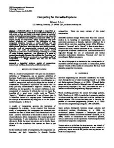
A real-time system [23].

From preliminary experimentation, appropriate initial tem, ranges from 100 to 140. Lower temperatures perature, results in premature convergence to a local minima, and higher temperatures produce numerous, potentially unnecessary iteraused is in the range of 0.70–0.90. tions. The value of cause the cooling temperature to be Smaller values of reduced too fast, which results in an insufficient random search process in each neighborhood, at each temperature step. The number of iterations per temperature step is an increasing , where temfunction: perature step, the same as above. This iteration function causes more iterations in the later stages of the search, at lower temperatures. With a higher number of iterations, near-optimal or optimal solutions are expected to be found. The constant 1.18 is a predefined value which works well for this particular problem. This number was obtained from our preliminary runs. Cost Constraint Consideration: For this paper, we consider solutions which satisfy the cost constraint. The search is limited to this feasible region, and neighbor moves are only to new values within the feasible region. In other work [22], we applied a penalty function to solutions which violate the constraints (i.e., nonfeasible solutions). Doing this, solutions with unsatisfied constraints can be considered with some penalties added to the reliability/cost functions. Conceptually, this approach allows the algorithm to explore new phases of the search space, which leads to promising solutions [11], [12]. Selection of New Neighborhood Solution: Only one subsystem is randomly selected to be perturbed at each iteration. A new hardware component and a software component for the selected subsystem are randomly chosen. Stopping Criterion: We terminate the optimization simulation when there is no improvement in the best solution within a specified number of iterations. Because the search space in these four optimization models/problems is not too large, we observe that, at the temperature step 50, satisfied solutions were found from the SA simulations. V. AN EXAMPLE SYSTEM AND COMPUTATIONAL RESULTS The reliability optimization models are now demonstrated on an example system, which is the real-time system shown in Fig. 3. The system [23] contains three network subsystems: Bessel, Bohr, and Fourier; and five processing subsystems: Galileo, Faraday, Halley, Kirchoff, and Ohm. Seven applications assigned to run on this system are labeled as applications

WATTANAPONGSAKORN AND LEVITAN: RELIABILITY OPTIMIZATION MODELS FOR EMBEDDED SYSTEMS WITH MULTIPLE APPLICATIONS

Fig. 4.

411

Applications running on the real-time system [23].

A, B, C, D, E, F, and G, which are audio processing applications. Each of the applications performs fetch-audio processing on one processing subsystem, and then the data is sent across a network to another processing subsystem to process the audio data. The mapping of each application onto the system platform is shown in Fig. 4. As a result, many hardware resources need to be shared among the applications. To make the problem more realistic, utilization functions are considered such that the component reliability is degraded when it is loaded by multiple applications. For this example, we initially perform system reliability optimization with cost constraints. Then, we perform system cost optimization with reliability constraints for multiple applications sharing the same hardware resources. Because each application consists of subsystems connected in series as shown in Fig. 4, the system reliability for each applica-

tion can be readily obtained, provided that each subsystem-reliability is known. Then, the reliability of the total system consisting of all applications can be calculated, where all the utilized subsystems are considered. Part of the available resources, subsystems Faraday and Bohr, are not used for any application. They are not considered in estimating the total system reliability. The reliability of the system is therefore calculated as

We assume that the utilization function for subsystem is given by is the number of applications . means that the running on subsystem , and subsystem is used by a single application. If more applications decreases. share the subsystem , the value of

412

IEEE TRANSACTIONS ON RELIABILITY, VOL. 53, NO. 3, SEPTEMBER 2004

TABLE I INPUT DATA: COMPONENTS AVAILABLE FOR MODELS 1–4

In this problem, for all and , , , which are in the range of the parameter values used in the published literature [2]. For each processing subsystem, many choices of software versions and hardware components are available, as shown in Table I. Each of the versions or components has a reliability and cost. As indicated in the table, the system has six subsystems (i.e., ); and each subsystem has three hardware component ), and four software versions available choices (i.e., ). However, the network subsystems (i.e., have fixed hardware components, so no choices are allowed (i.e., , and ). A. Reliability Optimization With Cost Constraints Reliability was optimized under various cost constraints for the embedded system using the optimization Models 1–4, using Simulated Annealing. As previously discussed, we randomly select an initial solution for each simulation run. For our relatively small size problems, a result for a model was obtained within a minute. Based on 10 runs for each model, with a specified cost constraint, at least 8 runs produce the same results, which represent our results, consisting of component and redundancy allocation information as well as the reliability of the system and applications, as captured in Table II. From the tables, the hardware component and software version allocations are shown as “h” and “s”, respectively. “2h” means that two identical hardware components are selected for the corresponding subsystem , choice . Similarly, “3h” means that three identical hardware components are selected. No identical software version is allowed for selection; therefore only one “s” is shown for a selected choice for a subsystem. Models 2–4 allow component redundancy, so there can be either one or three “s” for a subsystem in Models 2 and 3, and either one or

two “s” for a subsystem in Model 4. Similarly, there can be either one or three “h” for a subsystem in Model 3, either one or two “h” for a subsystem in Model 4, and one “h” for Models 1 and 2. These selections of “s” and “h” have to agree with the structures of redundant architectures, as shown in Fig. 2. We consider four cost constraints; 150, 200, 330, and 510. Fourier and Bessel network subsystems, which are assigned with fixed software and hardware component allocations, have no change in their components in the table. From the table, at a system cost of 150, no component redundancy is allowed, resulting in the same component allocations in all four models. The system reliability for this cost is 0.820 89, and the application reliabilities, as well as the corresponding total system cost, are shown at the lower half of the table. With a cost constraint of 200, higher system and application reliabilities can be obtained from all optimization models. Component redundancy is selected from Model 4, resulting in the maximum reliabilities provided at this cost, compared with the other three models. Models 1–3 provide the same component allocations and reliabilities for the system and applications. At this low cost, no redundancy can be obtained from these three models. With the no-redundancy option, using Model 1, the system cost of 330 gives the optimum component allocation. This is evident because there is no change in the component allocations and reliabilities when more system cost budget is available. The optimal allocations can be visualized as the results of selecting a software component and a hardware component with the highest reliability for each subsystem. When the cost budget is increased to 330, component redundancy is selected from all the models where it is applicable. For example, this is shown as redundant components selected for Models 2 and 4 for subsystem Galileo, and from Models 2–4 for subsystem Halley.

WATTANAPONGSAKORN AND LEVITAN: RELIABILITY OPTIMIZATION MODELS FOR EMBEDDED SYSTEMS WITH MULTIPLE APPLICATIONS

413

TABLE II RELIABILITY OF SYSTEM AND APPLICATIONS FROM MODELS 1–4 WITH COST CONSTRANTS 150, 200, 330 AND 510

With a cost budget of 510, the results indicate that more component redundancy can be selected for Models 2 –4, resulting in higher reliabilities obtained from each of the models, as compared to the results at the lower cost constraints. In summary, results from the tables show that, at higher cost budgets, the system and applications may be able to obtain higher reliabilities using better or more component choices, and component redundancy. Among these four optimization models, at any fixed cost constraint, the reliability result from Model 4 is the highest, and the reliability result from Model 3 is the second highest. This result agrees with data from published literature [2], [24], which indicates that at a certain architectures yield higher reliability cost, systems with the architectures. In other words, for the than those with the architectures cost same system reliability, systems with less than those with the architectures. In addition, with the same software choices and hardware choices, systems with architectures outperform the systems with the the architectures in terms of reliability.

B. Cost Optimization With Reliability Constraints In this section, we examine the case where, instead of optimizing reliability with cost constraints, cost becomes the objective function, and the system or application reliabilities are now the constraints. The optimizing model formulation is as follows.

414

IEEE TRANSACTIONS ON RELIABILITY, VOL. 53, NO. 3, SEPTEMBER 2004

TABLE III COMPONENT AND REDUNDANCY ALLOCATIONS UNDER RELIABILITY CONSTRAINTS

From the optimization model above, the total system cost is the summation of all the selected software and hardware components. This model allows a choice of component redunfor each subsystem. We chose to dant architecture further investigate the architecture choice, because it has potential to give better reliability results compared with and architecture, as was shown in the Section V-A. For a subsystem without redundancy, a single software version & a hardware component is selected; while redundancy, two different software versions & with

two hardware components with the same type & reliability are obtained. This model is the same as our Model 4, in the sense that both models consider the component redundancy architecture . They have the same assumptions for software and hardware components. Hardware components, with the same reliability values, are selected for a system if redundancy is obtained, while the selected software versions do not necessarily have the same reliability values. The constraints for this model are reliability requirements for some or all applications running on the common system platform, previously shown in Fig. 3. The reliability of each redundancy is subsystem is calculated using (3) if obtained. Otherwise, it is the product of the reliability of the selected software version and the hardware component. Using this model, we perform system cost optimization with multiple reliability constraints. We consider the four following different cases of reliability constraints. Case 1) Application A, B, C, D, E, and F, each requires reliability of 0.90 Case 2) Applications A, B, C, D, E, and F, each requires reliability of 0.92 Case 3) Applications A, B, C, D, E, and F each requires reliability of 0.95 Case 4) Applications A requires reliability of 0.95; and applications B, C, D, E, and F each requires reliability of 0.92. The optimization results were obtained for each case. The results were compared to investigate how the constraints affect the system cost, system reliability, and the reliability of other applications on the same system. We use the same cost and reliability data from Table I. From Table III, we see that, for Case 1, only the subsystem Galileo has redundant components allocated. For the other three cases, each has more subsystems with redundant components. This can be explained as an effect of the requirement constraints. Comparing all cases, Case 1 has the lowest reliability requirement, while Case 3 has the highest reliability

WATTANAPONGSAKORN AND LEVITAN: RELIABILITY OPTIMIZATION MODELS FOR EMBEDDED SYSTEMS WITH MULTIPLE APPLICATIONS

415

TABLE IV SYSTEM AND APPLICATION COSTS AND RELIABILITIES UNDER RELIABILITY CONSTRAINTS

requirement. To satisfy the higher requirement, component redundancy may be required. As a result, in Case 3, three of the four subsystems have redundant components. Cases 2 and 4 have the same selected components and redundancy, due to the relative similarity of the reliability requirements. If more choices of components are available for each subsystem, more suitable components could be selected. This could result in different component and redundancy allocations for the system in Cases 2 and 4. Table IV presents reliability results of the total system, , and each application. It shows that the satisfied total system costs for Cases 1, 2, 3, and 4 are 160, 180, 289, and 180, respectively. Compared with other cases, the system in Case 3 has the highest system cost due to the relatively high reliability requirements which are required. In contrast, the system in Case 1, with lowest reliability requirements, has the lowest cost. Since Cases 2 and 4 have the same component and redundancy allocations, they have the same system cost. The cost, however, is less than that required in Case 3, because less component redundancy is obtained, as shown in Table III. The results of the application reliabilities for each case, where reliability requirement constraints are required, are shown in bold in Table IV. VI. SUMMARY AND FUTURE WORK Based on our optimization results from the example problems, and previous research [22], it can be concluded that our reliability optimization models with the SA approach provide satisfactory reliability results while meeting the constraints. In our research, the SA algorithm was selected to demonstrate system reliability optimization or cost optimization techniques for embedded systems, because of its flexibility for various problem types with various constraints, and its efficiency in computation time. Similar to other researchers who have applied heuristic approaches to optimization models [11]–[13], [16], we chose the SA algorithm as the optimization approach even though it provides no guarantee of optimality. To potentially obtain better system reliability results, we plan to consider other heuristic techniques such as the Genetic Algorithm or the Tabu Search for system reliability optimizations as our future work. They give promising results to some reliability optimization models as presented in [11]–[13]. As future work, we also plan to consider hybrid fault-tolerant embedded system architectures such as a hybrid Recovery and -Version Programming model [25]. Block The model has a promising architecture to improve the total

system reliability with low cost, due to the combination of reliand the architectures. For this hyability from the can be embedded within an by brid architecture, applying an module to each version of the . Similarly, can be embedded within an . These types of hybrid architectures can be applied recursively to form many different multi-level hybrid fault-tolerant architectures. REFERENCES [1] J.-C. Laprie, J. Arlat, C. Beounes, and K. Kanoun, “Definition and analysis of hardware- and software-fault-tolerant architectures,” IEEE Computer, pp. 39–51, July 1990. [2] M. R. Lyu, Ed., Handbook of Software Reliability Engineering: McGraw-Hill, IEEE Computer Society Press, 1996, ch. 1–3, and 14. [3] R. K. Scott, J. W. Gault, and D. F. McAllister, “Fault-tolerant software reliability modeling,” IEEE Trans. Software Engineering, vol. SE-13, pp. 582–592, 1987. [4] M. S. Chern, “On the computational complexity of reliability redundancy allocation in a series system,” Oper. Res. Lett., vol. 11, pp. 309–315, 1992. [5] D. E. Fyffe, W. W. Hines, and N. K. Lee, “System reliability allocation and a computational algorithm,” IEEE Trans. Rel., vol. R-17, pp. 64–69, 1968. [6] Y. Nakagawa and S. Miyazaki, “Surrogate constraints algorithm for reliability optimization problems with two constraints,” IEEE Trans. Rel., vol. R-30, pp. 175–180, 1981. [7] N. Ashrafi and O. Berman, “Optimization models for selection of programs, considering cost & reliability,” IEEE Trans. Rel., vol. 41, pp. 281–287, 1992. [8] O. Berman and N. Ashrafi, “Optimization models for reliability of modular software systems,” IEEE Trans. Software Engineering, vol. 19, pp. 1119–1123, 1993. [9] N. Ashrafi and O. Berman, “Optimization models for selection of programs, considering cost & reliability,” IEEE Trans. Rel., vol. 41, pp. 281–287, 1992. [10] M. E. Helander, M. Zhao, and N. Ohlsson, “Planning models for software reliability and cost,” IEEE Trans. Software Engineering, vol. 24, pp. 420–434, 1998. [11] D. W. Coit and A. E. Smith, “Reliability optimization of series-parallel systems using a genetic algorithm,” IEEE Trans. Rel., vol. 45, pp. 254–260, 1996. [12] , “Adaptive penalty methods for genetic optimization of constrained combinatorial problems,” INFORMS. J. Computing, vol. 8, no. 2, pp. 173–182, 1996. [13] S. Kultural, B. A. Norman, D. W. Coit, and A. E. Smith, “Exploiting Tabu search memory in constrained problems,” INFORMS Journal of Computing, 2004, to be published. [14] C. R. Reeves and J. E. Beasley, Modern Heuristic Techniques for Combinatorial Problems. New York: Halsted Press, 1993, ch. 2. [15] Z. Michalewicz and D. Fogel, How to Solve it: Modern Heuristics: Springer Verilog, 1999, pp. 115–125. [16] R. W. Eglese, “Simulated annealing: A tool for operation research,” Eur. J. Oper. Res., vol. 46, no. 3, pp. 271–281, 1990. [17] R. L. Rardin, Optimization in Operations Research: Prentice Hall, 1998, pp. 690–694. [18] C. E. Ebeling, An Introduction to Reliability and Maintainability Engineering: McGraw-Hill, 1997, pp. 23–121. [19] D. E. Eckhardt and L. D. Lee, “A theoretical basis for the analysis of multiversion software subject to coincident errors,” IEEE Trans. Software Engineering, vol. 11, pp. 1511–1517, 1985.

416

IEEE TRANSACTIONS ON RELIABILITY, VOL. 53, NO. 3, SEPTEMBER 2004

[20] D. E. Eckhardt, A. K. Caglayan, J. C. Knight, L. D. Lee, D. F. McAllister, M. A. Vouk, and J. P. Kelly, “An experimental evaluation of software redundancy as a strategy for improving reliability,” IEEE Trans. Software Engineering, vol. 17, pp. 692–702, 1991. [21] J. B. Dugan, “Experimental analysis of models for correlation in multiversion software,” in Int. Symp. Software Reliability Engineering, Los Alamitos, CA, 1994, pp. 36–44. [22] N. Wattanapongsakorn, “Integrating Dependability Analysis and Optimization into the Distributed Embedded System Design Process,” Ph.D., School of Electrical Engineering, University of Pittsburgh, 2000. [23] S. Chatterjee, “Distributed Pipeline Scheduling: A Framework for Design of Large-Scale, Distributed, Heterogeneous Real-Time Systems,” Ph.D., School of Electrical and Computer Engineering, Carnegie Mellon University, 1996. [24] J. Xu and B. Randell, “Software fault tolerance” t=(n 1)-Variant programming,” IEEE Trans. Rel., vol. 46, pp. 60–68, 1997. [25] J. Wu, E. B. Fernandez, and M. Zhang, “Design and modeling of hybrid fault-tolerant software with cost constraints,” J. System Software, vol. 35, pp. 141–149, 1996.

0

Naruemon Wattanapongsakorn is an Assistant Professor in Computer Engineering at the King Mongkut’s University of Technology Thonburi (KMUTT), Thailand. She received the B.S. degree in Computer Engineering (1994), and the M.S. degree in Electrical Engineering (1995), both from The George Washington University, and Ph.D. degree in Electrical Engineering (2000) from the University of Pittsburgh. Her research interests include distributed system dependability analysis, optimization algorithms, embedded system modeling, software fault-tolerance, and statistical analysis of system reliability. She is a member of the IEEE, and the IEEE Reliability Society.

Steven P. Levitan is the John A. Jurenko Professor of Computer Engineering at the University of Pittsburgh. He received the B.S. degree from Case Western Reserve University (1972) and his M.S. (1979) and Ph.D. (1984), both in Computer Science, from the University of Massachusetts, Amherst. He worked for Xylogic Systems designing hardware for computerized text processing systems and for Digital Equipment Corporation on the Silicon Synthesis project. He was an Assistant Professor from 1984 to 1986 in the Electrical and Computer Engineering Department at the University of Massachusetts. In 1987 he joined the Electrical Engineering faculty at the University of Pittsburgh. His research interests include VLSI architectures, optoelectronic computing systems, parallel algorithm design, and HDL simulation and synthesis for VLSI. He is an Associate Editor of the ACM Transactions on Design Automation of Electronic Systems. He is Past Chair of the ACM Special Interest Group on Design Automation, a member of OSA, and a senior member of IEEE/CS.