Single Channel Source Separation with General Stochastic Networks Matthias Z¨ohrer and Franz Pernkopf Signal Processing and Speech Communication Laboratory Graz University of Technology, Austria
[email protected],
[email protected]
Abstract Single channel source separation (SCSS) is ill-posed and thus challenging. In this paper, we apply general stochastic networks (GSNs) – a deep neural network architecture – to SCSS. We extend GSNs to be capable of predicting a time-frequency representation, i.e. softmask by introducing a hybrid generative-discriminative training objective to the network. We evaluate GSNs on data of the 2nd CHiME speech separation challenge. In particular, we provide results for a speaker dependent, a speaker independent, a matched noise condition and an unmatched noise condition task. Empirically, we compare to other deep architectures, namely a deep belief network (DBN) and a multi-layer perceptron (MLP). In general, deep architectures perform well on SCSS tasks. Index Terms: general stochastic network, speech separation, speech enhancement, single channel source separation
1. Introduction Researchers have attempted to solve SCSS problems from various perspectives. In [1, 2] the focus is on model based approaches. Recently [3] approached the problem via structured prediction. In all cases a time-frequency matrix called ideal binary mask (IBM) is estimated from a mixed input spectogram X, separating X into noise and speech parts. In this case the underlying assumption is that speech is sparse, i.e. each time frequency bin belongs to one of the two assumed sources. Despite of the good results using deep models and binary masks [3], little attention has been payed to using a real valued mask i.e. softmask. This type of mask allows a more precise estimate of speech, leading to a better overall quality [4]. In this paper, we use the softmask in conjunction with deep learning i.e. we view SCSS as a regression problem. The success in deep learning originates from breakthroughs in unsupervised learning of representations, based mostly on the restricted Boltzmann machine (RBM) [5], auto-encoder[6, 7] and sparse-coding variants [8, 9]. These models in representation learning also obtain impressive results in supervised learning tasks, such as speech recognition, c.f. [10, 11, 12] and computer vision problems [13]. The latest development in object recognition is a form of noise injection during training, called dropout [14]. Often deep models are pre-trained by a greedy-layerwise procedure called contrastive divergence [5], i.e. a network layer learns the representation from the layer below by treating the latter as static input. Recently, a new training procedure for supervised learning, called walkback We gratefully acknowledge funding by the Austrian Science Fund under the project P25244-N15
training, was introduced [15]. The combination of noise, a multi-layer feed-forward neural network and walkback training leads to a new network architecture, the generative stochastic network (GSN) [16]. If trained with backpropagation, the model can be jointly pre-trained removing the need for a greedy-layerwise training procedure. Empirical results obtained in [15, 17] show that this form of joint pre-training leads to superior results on several image reconstruction tasks. However this technique has never been applied to supervised learning problems. In this paper, we use GSNs to learn and predict the softmask for SCSS. We introduce a new joint walkback training method to GSNs. In particular, we use a generative and discriminative training objective to learn the softmask to separate signal mixtures of the 2nd CHiME speech separation challenge [18]. We define four tasks: A speaker dependent (SD), a speaker independent (SI), a matched noise condition (MN) and an unmatched noise condition (UN) task. The GSN is compared to a deep belief network (DBN) [5] and a rectifier multi-layer perceptron (MLP) [19, 20]. GSNs perform on par with rectifier MLPs. Both slightly outperform a DBN i.e. the MLP achieved the best PESQ [21] score, namely 3.17 for the (SD) task, 3.30 for the (MN) task and 2.7 for the (UN) task. The GSN achieved the best PESQ score 2.72 on the (SI) task. This paper is organized as follows: Section 2 presents the mathematical background. Section 3 introduces four SCSS problems using the CHiME database. Section 4 presents experimental results of the GSN, the DBN and the recifier MLP and summarizes results. Section 5 concludes the paper and gives a future outlook.
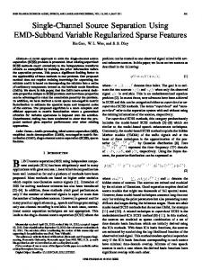
2. General Stochastic Networks Denoising autoencoders (DAE) [7] define a Markov chain, where the distribution P (X) is sampled to convergence. The transition operator first samples the hidden state Ht from a corruption distribution, and generates a reconstruction from the parametrized model, i.e the density Pθ2 (X|H). The resulting DAE Markov chain is shown in Figure 1.
Ht+1 Pθ 1
Ht+2 Pθ1
Pθ2
Xt+0
Ht+3 Pθ1
Pθ2
Xt+1
Ht+4
Pθ2
Xt+2
Pθ 1
Pθ1 Pθ2
Xt+3
Figure 1: DAE Markov chain.
Xt+4
A DAE Markov chain can be written as
Ht+1 ∼ Pθ1 (H|Xt+0 ) and Xt+1 ∼ Pθ2 (X|Ht+1 ),
(1)
where Xt+0 is the input sample X, fed into the chain at time step t = 0 and Xt+1 is the reconstruction of X at time step t = 1. Ht+0
Ht+1
Ht+2
Pθ1
Ht+3
Pθ1 Pθ2
Xt+0
Ht+4
Pθ1 Pθ2
Xt+1
Pθ1
Pθ1 Pθ2
Xt+2
Pθ 2
Xt+3
Xt+4
Figure 2: GSN Markov chain. In the case of a GSN, an additional dependency among the latent variables Ht over time is introduced in the network graph. Figure 2 shows the corresponding Markov chain, written as
Multiple hidden layers require multiple deterministic functions of random variables fθ ∈ {fˆθ0 , ..., fˆθd , fˇθ0 , ...fˇθd }. Figure 3 shows a Markov chain for a three layer GSN, inspired by the unfolded computational graph of a deep Boltzmann machine Gibbs sampling process. In the training case, alternatively even or odd layers are updated at the same time. The information is propagated both upwards and downwards for K steps. An example for this update process is given in Figure 3. In the even update (marked in 1 0 red) Ht+1 = fˆθ0 (Xt+0 ). In the odd update (marked in blue) 0 1 2 1 0 ˇ Xt+1 = fθ (Ht+1 ) and Ht+2 = fˆθ1 (Ht+1 ) for k = 0. In 1 0 2 0 ˆ the case of k = 1, Ht+2 = fθ (Xt+1 ) + fˇθ1 (Ht+2 ) and 3 2 0 1 Ht+3 = fˆθ2 (Ht+2 ) in the even update and Xt+2 = fˇθ0 (Ht+2 ) 2 1 1 3 and Ht+3 = hatfθ (Ht+2 ) + fˇθ2 (Ht+3 ) in the odd update. 1 0 2 In case of k = 2, Ht+3 = fˆθ0 (Xt+2 ) + fˇθ1 (Ht+3 ) and 3 2 0 1 2 ˆ ˇ Ht+4 = fθ (Ht+3 ) in the even update and Xt+3 = fθ0 (Ht+3 ) 2 1 3 1 2 ˆ ˇ and Ht+4 = fθ (Ht+3 ) + fθ (Ht+4 ) in the odd update. The cost function of a generative GSN can be written as
Ht+1 ∼ Pθ1 (H|Ht+0 , Xt+0 ) Xt+1 ∼ Pθ2 (X|Ht+1 ).
(2)
C=
K X
0 Lt {Xt+k , Xt+0 },
(3)
k=1
We express this chain with deterministic functions of random variables fθ ⊇ {fˆθ , fˇθ }. The density fθ is used to model Ht+1 = fθ (Xt+0 , Zt+0 , Ht+0 ), specified for some independent noise source Zt+0 . Xt+0 cannot be recovered exactly from Ht+1 . The function fˆθi is a back-probable stochasˆi ) with tic non-linearity of the form fˆθi = ηout + g(ηin + a noise processes Zt ⊇ {ηin , ηout } for layer i. The variable a ˆi is the activation for unit i, where a ˆi = W i Iti + bi with g as a non-linear activation function applied to a weight matrix W i and a bias bi . The input Iti denotes either the realization xit of observed sample Xti or the hidden realization hit of Hti . In general, fˆθi (Iti ) defines an upward path in a GSN i for a specific layer i. In the case of Xt+1 = fˇθi (Zt+0 , Ht+1 ) we specify fˇθi (Hti ) = ηout + g(ηin + a ˇi ) as a downward path in the network i.e. a ˇi = (W i )T Hti + (bi )T , using the transpose of the weight matrix W i and the bias bi respectively. This formulation allows to directly back-propagate the reconstruction log-likelihood log(P (X|H)) for all parameters θ ⊇ {W 0 , ..., W d , b0 , ..., bd } where d is the number of hidden layers. Figure 2 shows a GSN with a simple hidden layer, using two deterministic functions, i.e. {fˆθ0 , fˇθ0 }.
where Lt is a specific loss-function such as the mean squared error (MSE) at time step t. Optimizing the loss function by building the sum over the costs of multiple reconstructions is called walkback training [15, 16]. This form of network training is considerably more favorable than single step training, as the network is able to handle multi-modal input representations [15] if noise is injected during the training process. Equation 3 is specified for unsupervised learning of representations. In order to make a GSN suitable for a supervised learning task we introduce the output Y to the network graph. The cost function changes to L = log P (X) + log P (Y |X). The layer update-process stays the same, as the target Y is not fed into the network. However Y is introduced as an additional cost term. Figure 4 shows the corresponding network graph for supervised learning with red and blue edges denoting the even and odd network updates. 3 Lt {Ht+1 , Yt+0 }
3 Lt {Ht+2 , Yt+0 }
3 Ht+3
3 Ht+4
fˆθ2 3 Ht+3
fˆθ1
fˇθ2
1 Ht+1
fˆθ0
fˆθ1
fˆθ0
fˇθ2
fˆθ1
fˆθ0
2 Ht+2
fˆθ1 fˇθ1
1 Ht+3
fˇθ0
fˆθ2
2 Ht+4
fˇθ1
1 Ht+2
fˇθ0
fˆθ2
2 Ht+3
fˇθ1
fˆθ2
fˇθ2
fˆθ2
3 Ht+4
fˆθ2
2 Ht+2
fˇθ2
fˆθ0
fˆθ1
2 Ht+4
fˇθ1
fˆθ1
fˇθ1
fˆθ1
fˆθ1 1 Ht+1
fˆθ0
1 Ht+4
fˇθ0
2 Ht+3
fˇθ1
fˇθ0
1 Ht+2
fˇθ0
fˆθ0
1 Ht+3
fˇθ0
fˆθ0
1 Ht+4
fˇθ0
fˆθ0
fˇθ0
fˆθ0
fˆθ0
0 Xt+0
0 Xt+1
0 Xt+2
0 Xt+3
0 Xt+4
Xt+0
0 Lt {Xt+1 , Xt+0 }
0 Lt {Xt+2 , Xt+0 }
0 Lt {Xt+3 , Xt+0 }
0 Lt {Xt+4 , Xt+0 }
Figure 3: GSN Markov chain with multiple layers and backprob-able stochastic units.
0 Xt+0
0 Xt+1
0 Xt+2
0 Xt+3
0 Xt+4
Xt+0
0 Lt {Xt+1 , Xt+0 }
0 Lt {Xt+2 , Xt+0 }
0 Lt {Xt+3 , Xt+0 }
0 Lt {Xt+4 , Xt+0 }
Figure 4: GSN Markov chain for input Xt+0 and target Yt+0 with backprob-able stochastic units.
4. Experimental Results
We define the following cost function for a 3-layer GSN:
C=
λ K
K X
Lt {Xt+k , Xt+0 } +
k=1
K 1−λ X 3 Lt {Ht+k , Yt+0 } K −d+1
(4)
k=d
Equation 4 defines a non-convex multi-objective optimization problem, where λ weights the generative and discriminative part of C. Using the mean loss, as in this case, is not mandatory but allows an equal balance of both loss terms for λ = 0.5 with input Xt+0 and target Yt+0 scaled to the same range.
3. Experimental Setup The 2nd CHiME speech separation challenge database [18] consists of 34 speakers with 500 training samples each, and a validation- and test-set with 600 samples. Every training sample has a clean, a reverb speech signal, an isolated noise signal and a signal mixture of reverberated speech and noise. We performed the following experiments: A speaker dependent separation task (SD), a speaker independent separation task (SI), a matched noise separation task (MN), and an unmatched noise separation task (UN). The primary goal was to predict )| 513 bins of the softmask i.e. Y (t, f ) = |S(t,f|S(t,f , )|+|N (t,f )| where f and t are the time and frequency bins and N (t, f ) and S(t, f ) are the noise and speech spectograms. The time frequency representation was computed by a 1024 point Fourier transform using a Hamming window of 32ms length and a steps size of 10ms. Due to the lack of isolated noise signals needed to compute the softmask in the validation- and test set, disjoint subsets of the training corpus were used for training and testing. All experiments were carried out using 5 male and 5 female speakers using the Ids {1,2,3,5,6,4,7,11,15,16}. In all training cases, spectograms of reverberated noisy signals at dB levels of {-6, -3, ±0, +3, +6, +9} were used to train one model. In all test scenarios each model was evaluated separately for every single dB level. In the SD and SI task original CHiME samples were used as a data source. In the MN and UN task, CHiME speech signals were mixed with noise variants from the NOISEX [23] corpus i.e. the Ids {1,...,12} were chosen for training and test case of the MN task, whereas the Ids {1,...,12} and {13,..,17} were selected for the training and test set of the UN task respectively. This corresponds to [3], with the exception of using CHiME speech utterances instead of the TIMIT [24] speech corpus. Details about the task specific setup are listed in Table 1.
task
database
SD SI MN UN
CHiME CHiME CHiME, NOISEX CHiME, NOISEX
speakers 10 10 10 10
utterance/speaker train valid test 400 50 50 40 5 5 40 5 5 40 5 5
Table 1: Number of Utterances used for Training / Validation / Test.
In order to evaluate the GSN on the tasks defined in the previous section, the overall perceptual score (OPS), the artifact perceptual score (APS), the target related perceptual score (TPS) and the interference-related perceptual score IPS [23] are used. The range of this scores are in between 0 and 100, where 100 is the best. Furthermore, the source to interference ratio (SIR), the source to artifacts ratio (SAR) and the source to distortion ratio (SDR) [25], are selected. Apart from that, the PESQ [21] measure, the signal-to-noise-ratio Preference SNR = 10 log Preference-enhanced and the HIT-FA [26],[27] were computed. To test the significance of the results a pair-wise t-Test [28] with p = 0.05 was calculated in all experiments. Furthermore, the noisy truth scores were calculated in all experiments. A grid-search for an MLP over the layer sizes N × d with N ∈ {500, 1000, ..., 3000} neurons per layer and d ∈ {1, ..., 5} number of layers for F ∈ {1, 3, 5, 7} speech frames per timestep was performed to find the optimal network size. The same network configuration was used for all models for a fair evaluation. The input data was normalized to zero mean and unit variance. Stochastic gradient descent with an early stopping criterion of 100 epochs was selected as a training algorithm for all models. The DBN was pre-trained using contrastive divergence for 200 epochs using k = 1 steps. Both DBN and MLP were fine-tuned using a cross-entropy objective. The GSN was simulated using k = 5 steps with the novel walkback training method using a MSE objective. The GSN hyper-parameter λt+0 = 1 was annealed with λt+1 = λt+0 · 0.99 per epoch to simulate pre-training in a GSN. Due to the superior characteristics of rectifier functions reported in [19] and [29] rectifier gates were used in the MLP and GSN. A l2 regularizer with weight 1e−4 was used when training the MLP. All simulations were executed on a GPU with the help of the mathematical expression compiler Theano [30]. Table 2 summarizes the parameters of all models. model GSN MLP DBN
N ×d 1000x3 1000x3 1000x3
F 5 5 5
activation rectifier rectifier sigmoid
σ noise 0.1 -
l2 1e−4 1e−4 1e−4
Table 2: Network Model Parameters.
4.1. Experiment 1: Speaker Dependent Separation The performance of the deep models is shown in Figure 5. The recifier MLP slightly outperforms the DBN and GSN. A t-test between the MLP and the DBN showed statistical significant differences for all PESQ scores, the SNR and SDR score at 9dB and for all SIR scores except 9dB. In case of the GSN also all PESQ values, the SNR and SDR at 0dB and 9dB, the SIR scores bewtween 0dB - 9dB, and the IPS score at -6dB and -3dB are statistical significant. 4.2. Experiment 2: Speaker Independent Separation The results for the speaker independent separation task are shown in Figure 6. The GSN slightly outperforms the DBN and MLP in terms of SRD, SIR, SAR, OPS, APS and IPS scores. Also the best PESQ score of 2.72 at 9dB was obtained by the
3
PESQ
4
3
0 3 dB
6
40
0 3 dB
6
9
0
3 dB
0 3 dB
6
0 −20 −6 −3
9
0 3 dB
6
9
20
0 3 dB
6
60 −6 −3
9
0 3 dB
6
9
0 3 dB
6
9
3 dB
0 3 dB
6
9
0 3 dB
6
9
Figure 5: Experimental Results: Speaker Dependent Separation GSN (∧), DBN (∨), MLP (∗) and Noisy Truth (--).
9
−6
20
0 3 dB
6
0
0
3 dB
0 3 dB
6
0 −20 −6 −3
9
0 3 dB
6
20
0 3 dB
6
9
10 0 −6 −3
0 3 dB
6
9
0 3 dB
6
9
100
80 60 −6 −3
9
6
20
9
100
0 −6 −3
9
−3
20
40
40 20 −6 −3
6
−20 −6 −3
60
50 0 −6 −3
0
0 −20 −6 −3
100
80
0.02 −3
20
10
0.08
0.04
40 −6
9
20
0 −6 −3
100
6
9
0.06
SNR
0
0 −6 −3
−3
20
40 APS
60
20 −6 −3
20
−20 −6 −3
9
−6
6
50
OPS
SDR
SNR
0 −20 −6 −3
9
SAR
dB
20
6
TPS
3
SIR
0
3 dB
60
0.04 −3
IPS
45 −6
0
SAR
0.06
−3
70
MSE
0.08
50
OPS
1 −6
9
SIR
HITFA
6
IPS
3 dB
SDR
0
2
APS
−3
55
MSE
1 −6
TPS
2
HITFA
PESQ
4
0 3 dB
6
50 0 −6 −3
9
Figure 7: Experimental Results: Matched Noise Separation GSN (∧), DBN (∨), MLP (∗) and Noisy Truth (--). 4 PESQ
2
2
1 −6
3
0.2
40
0.1
35 −6
0.05
0 3 dB
6
40
0 3 dB
6
9
0 3 dB
6
0 3 dB
6
9
0 3 dB
6
9
6
6
9
−6
20
−3
0
3 dB
20
50
6
0 3 dB
6
9
0 3 dB
6
40
40
0 3 dB
6
9
0 −20 −6 −3
9
SAR
0 −20 −6 −3
60
9
20 −6 −3 0 3 dB
3 dB
SIR
SNR 0 3 dB
0
0 −20 −6 −3
10
0 −6 −3
0.02 −3
20
6
9
20
9
100
80 60 −6 −3
6
20
0 −6 −3
9
100
20 0 −6 −3
3 dB
0 −20 −6 −3
9
40 APS
60
20 −6 −3
0 −20 −6 −3
9
0
0.04
40 −6
0 3 dB
6
100
20 0 −6 −3
0 3 dB
6
9
0 3 dB
6
9
0 3 dB
6
9
100
80 60 −6 −3
10 0 −6 −3
9
TPS
6
−3
20
0.06
50
IPS
0 3 dB
−6
IPS
−20 −6 −3
9
0.08
60
OPS
SDR
0
6
20
SAR
3 dB
TPS
0
SIR
−3
9
9
0.15
20
6
dB
MSE
6
45
SNR
0
SDR
3 dB
HITFA
0
MSE
−3
50
OPS
−3
70
1 −6
HITFA
3
APS
PESQ
3
0 3 dB
6
9
50 0 −6 −3
9
Figure 6: Experimental Results: Speaker Independent Separation GSN (∧), DBN (∨), MLP (∗) and Noisy Truth (--).
Figure 8: Experimental Results: Unmatched Noise Separation GSN (∧), DBN (∨), MLP (∗) and Noisy Truth (--).
4.4. Experiment 4: Unmatched Noise Separation GSN. When comparing the GSN with the second best model, i.e. the MLP, the HIT-FA scores at dB levels of -6, -3, 6, 9 are statistically significant. Furthermore, the MSE scores at -6dB and 0dB, the SNR between -3dB - 9dB, the SDR between 0dB - 9dB, all SIR scores except 0dB and the IPS scores between -6dB - 3dB are statistically significant. 4.3. Experiment 3: Matched Noise Separation The results for the matched noise separation tasks are shown in Figure 7. The MLP outperforms both the DBN and GSN. The results are significant for all decibel [dB] levels for the HIT-FA, MSE, SNR, SDR, SIR, SAR, TPS and IPS (except 6dB, 9dB) scores when comparing the MLP with the DBN. The MLP only generated significantly better SNR and SDR scores compared to the GSN. In general, the MLP obtained the best overall results. However, this task uses the same 12 noise variants for training and testing [3]. Hence the model might learn a perfect representation of the noise patterns.
Figure 8 shows the simulation results of the unmatched noise separation task. Again the MLP achieved the best overall result. When comparing the DBN with the MLP differences in the all HIT-FA values and SNR values, except -6dB are statistically significant.
5. Conclusions In this paper, we analyzed deep learning models using the softmask. We empirically showed in four SCSS tasks that rectifier MLPs achieved a better overall performance than its deep belief counterpart. We also introduced a new hybrid generative-discriminative learning procedure for GSNs, removing the need for generative pre-training. Although, our new model was not able to outperform the rectifier MLP in all tasks, the GSN achieved the best overall result on a independent speaker source separation task. In future research we will therefore focus on new strategies to improve the performance of GSNs when applied to SCSS.
6. References [1] A. Ozerov, P. Philippe, R. Gribonval, and F. Bimbot, “One microphone singing voice separation using source-adapted models,” in Proceedings of IEEE Workshop on Applications of Signal Processing to Audio and Acoustics, Oct. 2005, pp. 90–93. [2] M. Stark, M. Wohlmayr, and F. Pernkopf, “Source-filter-based single-channel speech separation using pitch information,” IEEE Transactions on Audio, Speech, and Language Processing, vol. 19, no. 2, pp. 242–255, 2011.
[18] E. Vincent, J. Barker, S. Watanabe, J. Le Roux, F. Nesta, and M. Matassoni, “The second CHiME speech separation and recognition challenge: An overview of challenge systems and outcomes,” in Proc. ASRU 2013 Automatic Speech Recognition and Understanding Workshop, 2013. [19] X. Glorot, A. Bordes, and Y. Bengio, “Deep sparse rectifier neural networks,” in JMLR W&CP: Proceedings of the Fourteenth International Conference on Artificial Intelligence and Statistics, Apr. 2011.
[3] Y. Wang and D. Wang, “Cocktail party processing via structured prediction,” in Advances in Neural Information Processing Systems, F. Pereira, C. Burges, L. Bottou, and K. Weinberger, Eds. Curran Associates, Inc., 2012, vol. 25, pp. 224–232.
[20] D. E. Rumelhart, G. E. Hinton, and R. J. Williams, “Neurocomputing: Foundations of research,” J. A. Anderson and E. Rosenfeld, Eds. Cambridge, MA, USA: MIT Press, 1988, ch. Learning Internal Representations by Error Propagation, pp. 673–695.
[4] R. Peharz and F. Pernkopf, “On linear and mixmax interaction models for single channel source separation,” in IEEE International Conference on Acoustics, Speech, and Signal Processing, 2012, pp. 249–252.
[21] “ITU-T Recommendation P.862. Perceptual Evaluation of Speech Quality (PESQ): An Objective Method for End-To-End Speech Quality Assessment of Narrow-Band Telephone Networks and Speech Codecs,” Feb. 2001.
[5] G. E. Hinton, S. Osindero, and Y.-W. Teh, “A fast learning algorithm for deep belief nets.” Neural computation, vol. 18, no. 7, pp. 1527–1554, 2006.
[22] P. Smolensky, Information processing in dynamical systems: Foundations of harmony theory. MIT Press, 1986, vol. 1, no. 1, pp. 194–281.
[6] Y. Bengio, P. Lamblin, D. Popovici, and H. Larochelle, “Greedy layer-wise training of deep networks,” in Advances in Neural Information Processing Systems, B. Sch¨olkopf, J. Platt, and T. Hoffman, Eds. Cambridge, MA: MIT Press, 2007, vol. 19, pp. 153– 160.
[23] A. Varga and H. J. Steeneken, “Assessment for automatic speech recognition: Ii. noisex-92: A database and an experiment to study the effect of additive noise on speech recognition systems,” Speech Communication, vol. 12, no. 3, pp. 247–251, 1993.
[7] P. Vincent, H. Larochelle, Y. Bengio, and P.-A. Manzagol, “Extracting and composing robust features with denoising autoencoders,” in Proceedings of the 25th international conference on Machine learning. ACM Press, 2008, pp. 1096–1103. [8] H. Lee, A. Battle, R. Raina, and A. A. Y. A. Ng, “Efficient sparse coding algorithms,” Advances in Neural Information Processing Systems, vol. 19, no. 2, p. 801, 2007. [9] M. aurelio Ranzato, C. Poultney, S. Chopra, and Y. L. Cun, “Efficient Learning of Sparse Representations with an Energy-Based Model,” in Advances in Neural Information Processing Systems, B. Sch¨olkopf, J. Platt, and T. Hoffman, Eds. MIT Press, 2007, vol. 19, pp. 1137–1144. [10] G. E. Dahl, M. Ranzato, A. Mohamed, and G. E. Hinton, “Phone Recognition with the Mean-Covariance Restricted Boltzmann Machine,” in Advances in Neural Information Processing Systems, J. Lafferty, C. K. I. Williams, J. Shawe-Taylor, R. Zemel, and A. Culotta, Eds., 2010, vol. 23, pp. 469–477. [11] L. Deng, M. L. Seltzer, D. Yu, A. Acero, A. rahman Mohamed, and G. E. Hinton, “Binary coding of speech spectrograms using a deep auto-encoder.” in INTERSPEECH, T. Kobayashi, K. Hirose, and S. Nakamura, Eds. ISCA, 2010, pp. 1692–1695. [12] F. Seide, G. Li, and D. Yu, “Conversational speech transcription using context-dependent deep neural networks.” in INTERSPEECH. ISCA, 2011, pp. 437–440. [13] A. Krizhevsky, I. Sutskever, and G. E. Hinton, “ImageNet Classification with Deep Convolutional Neural Networks,” in Advances in Neural Information Processing Systems, F. Pereira, C. Burges, L. Bottou, and K. Weinberger, Eds. Curran Associates, Inc., 2012, vol. 25, pp. 1097–1105. [14] G. E. Hinton, N. Srivastava, A. Krizhevsky, I. Sutskever, and R. Salakhutdinov, “Improving neural networks by preventing coadaptation of feature detectors,” CoRR, vol. abs/1207.0580, 2012. [15] Y. Bengio, L. Yao, G. Alain, and P. Vincent, “Generalized Denoising Auto-Encoders as Generative Models,” in Advances in Neural Information Processing Systems, C. Burges, L. Bottou, M. Welling, Z. Ghahramani, and K. Weinberger, Eds. Curran Associates, Inc., 2013, vol. 26, pp. 899–907. [16] Y. Bengio, E. Thibodeau-Laufer, and J. Yosinski, “Deep generative stochastic networks trainable by backprop,” CoRR, vol. abs/1306.1091, 2013. [17] S. Ozair, L. Yao, and Y. Bengio, “Multimodal transitions for generative stochastic networks.” CoRR, vol. abs/1312.5578, 2013.
[24] J. S. Garofolo, L. F. Lamel, W. M. Fisher, J. G. Fiscus, D. S. Pallett, and N. L. Dahlgren, “Darpa timit acoustic phonetic continuous speech corpus cdrom,” 1993. [25] E. Vincent, R. Gribonval, and C. Fevotte, “Performance measurement in blind audio source separation,” Audio, Speech, and Language Processing, IEEE Transactions on, vol. 14, no. 4, pp. 1462– 1469, July 2006. [26] N. Li and P. C. Loizou, “Factors influencing intelligibility of ideal binary-masked speech: implications for noise reduction.” The Journal of the Acoustical Society of America, vol. 123, no. 3, pp. 1673–1682, 2008. [27] G. Kim, Y. Lu, Y. Hu, and P. C. Loizou, “An algorithm that improves speech intelligibility in noise for normal-hearing listeners.” The Journal of the Acoustical Society of America, vol. 126, no. 3, pp. 1486–1494, 2009. [28] W. S. Gosset, “The probable error of a mean,” Biometrika, vol. 6, no. 1, pp. 1–25, March, originally published under the pseudonym “Student”. [29] V. Nair and G. E. Hinton, “Rectified linear units improve restricted boltzmann machines,” Proceedings of the 27th International Conference on Machine Learning, pp. 807–814, 2010. [30] J. Bergstra, O. Breuleux, F. Bastien, P. Lamblin, R. Pascanu, G. Desjardins, J. Turian, D. Warde-farley, and Y. Bengio, Theano: A CPU and GPU Math Compiler in Python, 2010, no. Scipy, pp. 1–7.