complex spectral profile is decomposed into a sum of several simple ripple spectra, then the unit response to the complex profile must equal the sum of the ...
Representation of Complex Dynamic Spectra in Auditory Cortex Jonathan Z. Simon, Didier A. Depireux and Shihab A. Shamma Institute for Systems Research & Electrical Engineering Department University of Maryland, College Park, MD 20742, U.S.A.
1. Introduction Recent neurophysiological experiments have shed new light onto how various sound features are encoded and organized in the primary auditory cortex (AI). One such feature is the envelope of broadband acoustic spectra, or spectral profile, the most important physical correlate of timbre (Plomp 1976). To determine how AI units represent complex dynamic profiles, it is essential to measure their spectro-temporal response field (STRF). This function is analogous to the receptive field of visual neurons in that it reflects the strength and dynamics of the unit responses to tones at different frequencies. A more traditional response measure of auditory units is the “response area”, defined roughly as the range of tone frequencies and intensities that just elicit excitatory or inhibitory responses. The response area is only useful as a qualitative predictor of a unit’s responses to arbitrary broadband spectra; its measurements is also significantly affected by a host of experimental difficulties and nonlinear factors that render estimates of parameters such as bandwidth and asymmetry quantitatively inaccurate (Shamma 1993, Shamma et al. 1995a, Nelken et al. 1994). To circumvent some of these problems, we have used new techniques to measure the spectral and dynamic properties of response areas in AI (Schreiner and Calhoun 1995, Shamma et al. 1995a). The stimuli and techniques—adapted from vision research (De Valois 1990) and from psychoacoustic studies (Green 1986, Hillier 1991, Summers and Leek 1994)— apply linear system theory to measure the response area of cortical units. Specifically, they employ broadband spectra with sinusoidally modulated profiles against the logarithmic frequency axis—or ripples—shown in Fig.1. By varying the ripple density (or frequency), amplitude, and drift velocity, one can measure a transfer function to such rippled spectra, and from it by an inverse Fourier transform obtain the STRF. A fundamental assumption of these techniques (reviewed briefly below) is that the responses to such broadband stimuli are substantially linear with respect to spectral profiles, that is they satisfy the superposition principle. This principle means that if a complex spectral profile is decomposed into a sum of several simple ripple spectra, then the unit response to the complex profile must equal the sum of the responses to each of these ripples. Superpostion has been validated using both stationary (Shamma et al. 1995a,b) and dynamic spectra that can be decomposed into any combination of downward moving ripples (Kowalski et al. 1996a, b).
Natural spectra such as speech, music, and various natural sounds are composed of both downward and upward moving ripples. Consequently, linearity (or superposition) must be validated for both directions of moving ripples. Furthermore, if linearity holds, we can derive unit STRFs from complete measurements of the transfer functions for ripples moving in both directions, followed by a 2-dimensional inverse Fourier transform.
Ripple Spectrogram
*
1 .5 .250
Time (ms)
250 0
STRF
Expected Response
=
8 4 2
0
50 100 150 200 250 0 Time (ms)
Time (ms)
250
Figure 1 Computing responses with STRF. Left: The ripple spectral profile consists of 101 tones equally spaced along the log. frequency axis, spanning 5 octaves (e.g., 0.25–8 kHz). The sinusoidally modulated envelope has a ripple density or frequency (Ω) given in units of cycles/octave; its constant velocity ω is defined as the number of ripple cycles traversing the lower edge of the spectrum per second (Hz). Middle: The response of a unit is deduced from its STRF shown here against the tonotopic axis with white representing postive amplitudes and black negative ones. Note the STRF is a function of time, and can be convolved with the input spectrogram to compute the expected response on the Right.
When dealing with both the temporal and spectral aspects of the responses, an important issue is the separability of these two dimensions, i.e., whether these response properties can be measured independently of each other. Without separability, transfer functions must be measured at all combinations of velocities and ripple densities, an impractical proposition given the extended times needed to hold a unit. With separabiltiy, it is sufficient instead to measure the temporal transfer function at one ripple density, and the spectral transfer function at one velocity; the complete transfer function is then taken as the product of these two one-dimensional transfer functions. In previous investigations using downward moving ripples (Kowalski et al. 1996a,b), it was demonstrated that the temporal and spectral transfer functions are indeed separable. This is because predictions of responses to various combinations of rippled spectra could be made from transfer functions measured at the best ripple velocity and ripple density only. Here, the notion of separability is extended to take into account both directions of moving ripples. To validate it, we shall assume that the complete spectrotemporal transfer function is quadrant separable, i.e., is the product of transfer functions measured at one ripple velocity and density, in each direction. We then proceed to derive the corresponding unit’s STRF, and to predict the responses to various combination of complex dynamic spectra composed of ripples moving in both directions. Fair predictions of responses to these spectra is taken as a validation of both the linearity and separability of the system.
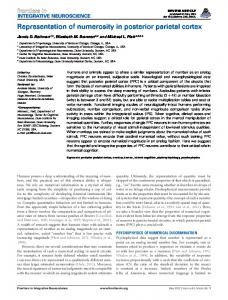
2. Methods The data used here were collected from AI of 2 Ketamine/Xylazine anesthetized domestic ferrets (Mustela putorius). Details of the surgery are as in (Shamma et al 1993). Moving ripples can be used to measure the temporal and ripple transfer function of cells, and hence derive their STRFs (Kowalski et al 1996a,b). The basic procedure is summarized here for ripple transfer function measurements. Fig.2 illustrates the response to moving ripples at a fixed ω = 8 Hz, and ripple frequency Ω from –1.6 to +1.6 cycles/octave (Fig.2A), i.e. upwards and downwards moving ripples. The magnitude and phase of the synchronized response at each Ω is derived and plotted as the magnitude and phase of the ripple transfer function Tω (Ω) (= Tω (Ω) e jΦω ( Ω ) ) (Fig.2B). The temporal transfer function TΩ(ω) are measured similarly, with the result shown in Fig 2C.
A Ripple Frequency (cyc/oct)
Ripple Velocity = 8 Hz
219/34a04
75 dB
Time (ms)
10 0 -1.6 0 1.6 Ripple Freq.
C 40 Ω = 0.4 c/o
-1.6 0 1.6 Ripple Freq.
20
2π π 0 −π
Phase Φ(ω)
20
2π π 0 −π
|TΩ(ω)|
ω = 8 Hz
Phase Φ(Ω)
30
|Tω(Ω)|
B
0 -24 0 24 Ripple Velocity
-24 0 24 Ripple Velocity
Figure 2 Transfer function measurements using moving ripples. A: Raster responses to a ripple moving at ω = 8 Hz with ripple frequencies Ω = –1.6 to 1.6 cycle/octave (or, equivalently, ripples moving at ω = 8 Hz with ripple frequencies Ω = 0 to 1.6 cycle/octave, and ripples moving at ω = –8 Hz with ripple frequencies Ω = 0.2 to 1.6 cycle/octave). B, C: The amplitude and phase of the fitted responses as a function of Ω and ω. A straight line fit of the phase data points is also shown.
The transfer functions Tω (Ω) and TΩ (ω ) are valid at one ripple frequency or velocity, as indicated by the subscripts ω and Ω. In principle, one must measure the two dimensional transfer function at all Ω and ω within each quadrant and compute a two dimensional STRF from the inverse transform. However, if we assume that, apart from a scale change, these functions remain unchanged over the most responsive range of Ω and ω , the temporal and ripple transfer functions can be treated as separable from each other, and measured at one Ω and ω , respectively.
There is a stronger (and more strict) notion of separability, independent of direction, i.e., applying uniformly across all quadrants (McLean and Palmer 1994, Watson and Ahumada 1985). This full separability occurs if the responses to downward and upwardmoving ripples are identical, implying a symmetric transfer function about the ω axis, and a symmetric STRF. These issues have already been the subject of theoretical and experimental studies in visual cortex, where quadrant-separability and a significant measure of linearity have been demonstrated (McLean and Palmer 1994). For a fully separable unit, the transfer function is a direct product T (Ω, ω ) = T (Ω)T (ω ) = T (Ω) e jΦ ( Ω ) T (ω ) e jΦ (ω ) . For a unit that is only quadrant separable, the transfer function is a sum of direct products for the right quadrants on the Ω−ω plane: T (Ω, ω ) = T± (Ω)T± (ω ), ± ω > 0, Ω > 0. Fig.3 illustrates the full STRF obtained from the inverse Fourier transform of the compound transfer function T (Ω, ω ) for three units. Apparent structure in the plot far away from the main body of the STRF are simply due to aliasing and noise effects. The STRF example in the middle panel is asymmetric with strong inhibition from the high frequency side. The unit in the third panel is almost fully separable. as can be seen from the spectral symmetry of its STRF at all times. Frequency (kHz)
8 4
.25
0 50 100 150 200 250 0 Time (ms)
50 100 150 200 250 0 Time (ms)
218/17a
.5
219/19a
1
219/34a
2
50 100 150200 250 Time (ms)
Figure 3 Examples of STRFs. Left: Response field computed from the inverse fourier transform of the full twodimensional transfer function of the unit in Figs.2 and 3. Middle and Right: Two more examples of a highly asymmetric STRF (middle) and a relatively broad bandwidth and slow symmetric STRF (right)
A periodic stimulus composed of a linear sum of ripples of different ripple frequencies and velocities is predicted to give a response which is a linear sum of sinusoids with amplitudes and phases weighted by the transfer fucntion T (Ω, ω ) = T (Ω, ω ) e jΦ ( Ω,ω ) . Applying such superposition to predict responses to complex stimuli is only meaningful if the system is essentially linear; so accurate predictions are a verification of linearity. Furthermore, the transfer function is calculated under the assumption of (quadrant) separability, so accurate predictions are also a verification of separability. Predictions can equivalently be made by a simple convolution of the STRF with the spectrogram of the stimulus as illustrated in Fig.4. In each case, the predicted waveform is plotted together with the response for visual comparison. The scale of the predicted waveform is arbitrary; however, its (zero) baseline is set at the rate of firing of the stationary stimulus at ω=0 in Fig.2C. Three more examples of predictions with multiple ripples are shown in Fig.4B.
*
.5
Prediction
.5
50 0 -50 50
100
150
Time (ms)
0
-50 0
50 100 150 200 250
0
50
100
200 250
50 0 -50 0
20
40
60
Time (ms)
150
200
250
Time (ms)
Response − Baseline 218/17A08.A1(6)
B
0
1
.25 50 100 150 200 250
50
2
80
100 120
50
219/34A07.A1(7)
1
4
218/17A08.A1(13)
2
Prediction Response − Baseline
8
219/34A07.A1(11)
4
.25 0
STRF Frequency (kHz)
8
=
Frequency (kHz)
A Stimulus Spectrogram
0
-50 0
50
100 150
200
250
Time (ms)
Figure 4 Predictions of the responses to complex dynamic spectra using the STRF. (A) The predicted response is computed by a convolution (along the time dimension) of the STRF with the spectrogram. The stimulus shown is composed of two ripples (0.4 c/o at 12 and –4 Hz). Same cell as in Fig.2. The predicted waveform (dashed line) is juxtaposed against the actual response (solid line) over one period of the stimulus. (B) Three additional examples of predictions using: (right and left panels) three ripples (0.4 c/o at 12,–4 Hz, and 0.2 c/o at –8 Hz) in 2 units; (middle panel) two ripples (0.6 c/o at –8 Hz, and 0.2 c/o at 24 Hz) for the same unit as the left panel.
3. Results Recordings so far have been made from 70 units in 2 animals. Many different types of STRFs have been observed as illustrated in Fig.3. They include symmetric (left and right panels) and asymmetric (middle panel), slow (right panel) and fast dynamics (left panel). We have not obtained yet an large enough sample of units to describe the statistical distribution of these properties in AI. AI responses to spectra composed of a few ripples can be reasonably well predicted from responses to single ripples by applying the superposition principle. This is shown earlier in Fig.4 using 2 and 3 ripple stimuli. Fig.5 illustrates additional examples on dynamic spectra composed of up to 16 moving ripples with different velocities, phases, and ripple frequencies. In all cases, predicted responses assuming linearity and quadrantseparability, compare well with those measured experimentally.
4. Discussion Linearity and separability are validated by the successful prediction of responses using the superposition principle and spectro-temporal transfer functions measured at one
velocity and ripple density. These properties have allowed us to derive STRFs for all units recorded, illustrating their diverse and complex structure.
2
2
1
*
0.25
= 219/26c
1
0.5 0
8
0.25 200 400 600 800 1000 0 8
4
4
2
2
1
*
0.5
0.5
0.25
20
200
0.25 200 400 600 800 1000 0
time (ms)
0
−20 0
400
100
200
300
time (ms)
400
500
400
500
Prediction Response – baseline 20
=
1
0
219/26c08.a1(2)
4
Prediction Response – baseline
200
400
time (ms)
219/26c08.a1(3)
4
0.5
frequency (kHz)
Spectro-Temporal RF 8
219/26c
frequency (kHz)
Stimulus Spectrogram 8
0
−20 0
100
200
300
time (ms)
Figure 5 Predicting the final response to large combinations of moving ripples in the same unit. A: Spectrograms of the stimulus, along with the ripple content. B: STRF of the cell (computed as described in Fig.5). All other details of the figure are as in Fig.4.
Linearity and separability simplify enormously the measurement and prediction of responses to complex dynamic spectra and reflect certain fundamental operational principles of the auditory, and perhaps other sensory systems. The persistence of response linearity to broadband stimuli suggest that the operative nonlinearities are those that do not destroy the basic linear character of the responses, such as threshold, half-wave rectification, and saturation in the early auditory stages. These limit significantly the dynamic range of the linear responses to ripple stimuli, but do not severely distort the overall gross shape of the responses (Shamma et al, 1995a; Kowalski et al, 1996a). It should be emphasized here, however, that all ripple stimuli are broadband in nature, and hence response linearity cannot be confirmed for narrowband stimuli such as stationary, AM, or FM tones. At first glance, the finding that separability holds for complex dynamic spectra is surprising, given the intertwining of temporal and spectral processing along the auditory pathway up to the cortex. One possible implication of this finding is that cortical temporal and spectral processing occur as two essentially separate sequential stages. In such a model, the first stage would have a purely spectral transfer function, followed by temporal filtering in the second stage. The overall spectro-temporal transfer function
would then be the product of the two transfer functions. This model is plausible if one assumes that response area shape (or the spectral cross-section of the STRF), e.g., asymmetry and bandwidth, is due to the organization of the thalamic (MGB) input projections to the AI or earlier stages. The slow temporal responses (rates mostly under 12 Hz) are likely to be related to the cortico-thalamic feedback loops. It is also likely that visual and other sensory pathways share the linearity and separability since none of the above physiological features are unique to AI. 5. Acknowledgment This work is supported by grants from the Office of Naval Research and the National Science Foundation (# NSFD CD 8803012). We thank David Klein and Nikos Kanlis for help in the recordings. 6. References C. Blackburn and M. Sachs (1990) The representation of the steady-state vowel /e/ in the discharge patterns of cat anteroventral cochlear nucleus neurons, J. Neurophysiol. 63 1191-1212 R. De Valois and K. De Valois (1990) Spatial Vision, Oxford University Press D.M. Green (1986), ‘Frequency’ and the detection of spectral shape change, in Auditory Frequency Selectivity, editors B.C.J. Moore and R.D. Patterson, Plenum Press, Cambridge 351-359 N. Kowalski, D. Depireux and S. Shamma (1996a) Analysis of dynamic spectra in ferret AI: Characteristics of single unit responses to moving ripple spectra, J. Neurophysiology 76 (5) 35033523 N. Kowalski, D. Depireux and S. Shamma (1996b) Analysis of dynamic spectra in ferret AI: Prediction of singl unit responses to arbitrary dynamic spectra, J. Neurophysiology 76 (5) 3524-3534 J. McLean and L. Palmer (1994) Organization of simple cell responses in the three-dimensional frequency domain, Visual Neuroscience (11) 295-306 I. Nelken, Y. Prut, E. Vaadia and M. Abeles (1994) Population responses to multifrequency sounds in the cat auditory cortex: One- and two-parameter families of sounds, Hear. Res.(72) 206-222 R. Plomp, 1976 Aspects of tone sensation, Academic Press, New York C. Schreiner and B. Calhoun (1995) Spectral envelope coding in cat AI, J. Aud. Neuroscience, (1) 39-61 S. Shamma, J. Fleshman, P. Wiser and H. Versnel (1993) Response Area Organization in the Ferret Primary Auditory Cortex, J. Neurophys. 69(2) 367-383 S. Shamma, H. Versnel and N. Kowalski (1995a) Ripple Analysis in the Ferret Auditory Cortex: I. Response Characteristics of Single Units to Sinusoidally Rippled Spectra, J. Auditory Neuroscience (1) 233-254 S. Shamma and H. Versnel (1995b) Ripple Analysis in the Ferret Primary Auditory Cortex. II:. Prediction of Unit Responses to Arbitrary Spectral Profiles, J. Auditory Neuroscience (1) 255-270 V. Summers and M. Leek (1994), The internal representation of spectral contrast in hearing-impaired listners, J. Acoust. Soc. Am.95(6) 3518-3528 A. Watson and A. Ahumada (1985) Model of human visual motion sensing J. Opt. Soc. Am. A2 322-342