Hindawi Publishing Corporation Mathematical Problems in Engineering Volume 2014, Article ID 710952, 7 pages http://dx.doi.org/10.1155/2014/710952
Research Article Robust 𝐻∞ Filtering for Networked Control Systems with Random Sensor Delay Shenping Xiao, Liyan Wang, Hongbing Zeng, Lingshuang Kong, and Bin Qin School of Electrical and Information Engineering, Hunan University of Technology, Zhuzhou 412007, China Correspondence should be addressed to Shenping Xiao; xsph
[email protected] Received 4 December 2013; Accepted 2 February 2014; Published 19 March 2014 Academic Editor: Huaicheng Yan Copyright © 2014 Shenping Xiao et al. This is an open access article distributed under the Creative Commons Attribution License, which permits unrestricted use, distribution, and reproduction in any medium, provided the original work is properly cited. The robust 𝐻∞ filtering problem for a class of network-based systems with random sensor delay is investigated. The sensor delay is supposed to be a stochastic variable satisfying Bernoulli binary distribution. Using the Lyapunov function and Wirtinger’s inequality approach, the sufficient conditions are derived to ensure that the filtering error systems are exponentially stable with a prescribed 𝐻∞ disturbance attenuation level and the filter design method is proposed in terms of linear matrix inequalities. The effectiveness of the proposed method is illustrated by a numerical example.
1. Introduction Networked control systems (NCSs) which are new control systems where sensor-controller and controller-actuator signal link is through a real time network [1]. Because of the advantages, such as convenient fault diagnosis, low cost, and simplicity, the NCSs have been widely applied in many application areas such as industrial automation, remote process, and manufacturing plants. However, the insertion of the communication network may cause time delay, so the signal transferred in NCSs loses the stationary, integrity, and determinacy, which makes the analysis of NCSs become complicate. Therefore, increasing attention has been paid to the study of networked control systems (see, e.g., [2–6] and references therein). On the other hand, the filtering problem for NCSs has attracted constant research [7–11] since it is important in control engineering and signal processing. In [7], the 𝐻∞ filtering for NCSs with multiple packet dropouts is considered. The problem of designing 𝐻∞ filter design for a class of discrete nonlinear NCSs with stochastic time-varying delays and missing measurements is addressed in [9], where sector nonlinearities and parameter uncertainties are also studied. In [10], by using a stochastic sampled-data approach, the problem of distributed 𝐻∞ filtering in sensor networks is considered. And distributed average filtering for sensor
networks with sensor saturation is designed by averagely fusing the information of each local node in [11]. However, there are few literatures to analyze the problem of 𝐻∞ filtering for continuous-time NCSs with random sensor delay, which motivates the present study. In this paper, a delay-dependent 𝐻∞ performance analysis result is derived for the filtering error system and a new random sensor delay model with stochastic parameter matrix is proposed. Combining the reciprocally convex combination technique in [12] and employing Wirtinger’s inequality approach, new criteria are derived for 𝐻∞ performance analysis, which reduces the conservatism. Based on the derived criteria for 𝐻∞ performance analysis, the novel 𝐻∞ filter criteria are obtained in terms of LMIs. Finally, a numerical example is presented to show the effectiveness of the proposed approach.
2. Problem Description Consider the following networked control systems: 𝑥̇ (𝑡) = 𝐴𝑥 (𝑡) + 𝐵𝑤 (𝑡) , 𝑦 (𝑡) = 𝐶𝑥 (𝑡) , 𝑧 (𝑡) = 𝐿𝑥 (𝑡) ,
(1)
2
Mathematical Problems in Engineering
where 𝑥(𝑡) ∈ 𝑅𝑛 and 𝑦(𝑡) ∈ 𝑅𝑚 are the state and measurable output vector, respectively. 𝑧(𝑡) ∈ 𝑅𝑞 is the signal to be estimated and 𝑤(𝑡) ∈ 𝑅𝑝 is the external disturbance signal belonging to 𝐿 2 [0, ∞]. 𝐴, 𝐵, 𝐶, and 𝐿 are known matrices with appropriate dimensions. Consider the following filter for the estimation of 𝑧(𝑡): 𝑥𝑓̇ (𝑡) = 𝐴 𝑓 𝑥𝑓 (𝑡) + 𝐵𝑓 𝑦̃ (𝑡) , 𝑧𝑓 (𝑡) = 𝐿 𝑓 𝑥𝑓 (𝑡) , 𝑛
̃ ∈ 𝑅 are the filter’s state and where 𝑥𝑓 (𝑡) ∈ 𝑅 and 𝑦(𝑡) input vector, respectively. 𝑧𝑓 (𝑡) ∈ 𝑅𝑞 is the estimated output. 𝐴 𝑓 , 𝐵𝑓 , and 𝐿 𝑓 are the filter matrices to be designed. In the actual networked control systems, the measured ̃ ∈ 𝑅𝑚 may or may not experience sensor delay, output 𝑦(𝑡) which can be described by two random events:
Event 2 : 𝑦 (𝑡) experiences sensor delay.
𝑃 {Event 2} = 1 − 𝜐0 .
(4)
if Event 1 occurs, if Event 2 occurs.
𝑃 {𝜐 (𝑡) = 0} = 𝐸 {1 − 𝜐 (𝑡)} = 1 − 𝜐0 ,
(5)
(6)
(7)
where 𝜏(𝑡) stands for time-varying delay which satisfies 𝜏𝑚 ⩽ 𝜏(𝑡) ⩽ 𝜏𝑀. 𝑇 Define 𝜉(𝑡) = [𝑥𝑇 (𝑡) 𝑥𝑓𝑇 (𝑡)] and 𝑒(𝑡) = 𝑧(𝑡) − 𝑧𝑓 (𝑡); then the filtering error system can be described as follows: ̃ (𝑡) + 𝜐0 𝐵̃𝑑 𝜉 (𝑡) + (1 − 𝜐0 ) 𝐴 ̃𝑑 𝐸𝜉 (𝑡 − 𝜏 (𝑡)) 𝜉 ̇ (𝑡) = 𝐴𝜉 ̃ (𝑡) , + 𝐵𝑤
̃ = [𝐿 𝐿 𝑓 ] . 𝐿
Our aim in this paper is to design a robust 𝐻∞ filter in the form of (8) such that (1) system (1) is robustly exponentially stable, subject to 𝑤(𝑡) = 0, (2) under zero initial condition and for the disturbance attenuation level 𝛾, the controlled output 𝑒(𝑡) satisfies ‖𝑒(𝑡)‖2 ⩽ 𝑟‖𝑤(𝑡)‖2 for 𝑤(𝑡) ∈ 𝐿 2 [0, ∞], 𝑤(𝑡) ≠ 0. Lemma 1 (see [13]). For any positive matrix 𝑅, and for differentiable signal 𝑥 in [𝛼, 𝛽] → 𝑅𝑛 , the following inequality holds: 𝑇
𝑥 (𝛽) 𝑥 (𝛽) 1 [ 𝑥 (𝛼) ] 𝑊 (𝑅) [ 𝑥 (𝛼) ] , ∫ 𝑥̇ (𝑢) 𝑅𝑥̇ (𝑢) 𝑑𝑢 ⩾ 𝛽−𝛼 𝛼 [ 𝜒 ] [ 𝜒 ] (10) 𝛽
𝑇
𝛽 1 ∫ 𝑤 (𝑢) 𝑑𝑢, 𝛽−𝛼 𝛼
(11)
𝑅 −𝑅 0 𝑅 𝑅 −2𝑅 𝜋2 [ ∗ 𝑅 −2𝑅] . 𝑊 (𝑅) = [∗ 𝑅 0] + (12) 4 ∗ ∗ 4𝑅 ∗ ∗ 0 [ [ ] ] Lemma 2 (see [14]). For any positive matrix 𝑀 > 0, scalar 𝑟 > 0, and a vector function 𝑤 : [0, 𝑟] → 𝑅𝑛 such that the 𝑟 integration ∫0 𝑤(𝑠)𝑇 𝑀𝑤(𝑠)𝑑𝑠 is well defined, then 𝑟
𝑟
0
0
𝑇
𝑟
0
(13)
Lemma 3 (see [12]). Let 𝐹1 , 𝐹2 , 𝐹3 , . . . , 𝐹𝑁 : 𝑅𝑚 → 𝑅 have positive values for arbitrary value of independent variable in an open subset 𝑊 of 𝑅𝑚 . The reciprocally convex combination of 𝐹𝑖 (𝑖 = 1, 2, . . . , 𝑁) in 𝑊 satisfies min
𝑙 𝑙 l 𝑙 1 ∑ 𝐹𝑖 (𝑡) = ∑𝐹𝑖 (𝑡) + max ∑ ∑ 𝑊𝑖,𝑗 (𝑡) 𝑖=1 𝜂𝑖 𝑖=1 𝑖=1 𝑗=1,𝑗 ≠ 𝑖
subject to
{𝜂𝑖 > 0, ∑𝜂𝑖 = 1, 𝑊𝑖,𝑗 (𝑡) : 𝑅𝑚 → 𝑅,
𝑁
𝑖=1
(8) ̃ (𝑡) , 𝑒 (𝑡) = 𝐿𝜉
(9)
𝑟 (∫ 𝑤(𝑠)𝑇 𝑀𝑤 (𝑠) 𝑑𝑠) ⩾ (∫ 𝑤 (𝑠) 𝑑𝑠) 𝑀 (∫ 𝑤 (𝑠) 𝑑𝑠) .
where 𝜐0 is a known constant on [0, 1]. Considering the random sensor delay, we suppose that the corresponding measurement is defined as 𝑦̃ (𝑡) = 𝜐0 𝑦 (𝑡) + (1 − 𝜐0 ) 𝑦 (𝑡 − 𝜏 (𝑡)) ,
̃𝑑 = [ 0 ] , 𝐴 𝐵𝑓 𝐶
𝜒=
By using Bernoulli distributed sequence, the variable 𝜐(𝑡) can be assumed to follow an exponential distribution of switching, which satisfies 𝑃 {𝜐 (𝑡) = 1} = 𝐸 {𝜐 (𝑡)} = 𝜐0 ,
𝐸 = [𝐼 0] ,
where
Define a stochastic variable 𝜐(𝑡): 1, 𝜐 (𝑡) = { 0,
𝐵 𝐵̃ = [ ] , 0
Throughout this paper, we use the following lemmas. (3)
Assume that the occurrences probability of the above given event can be described as the following formula: 𝑃 {Event 1} = 𝜐0 ,
0 0 ], 𝐵̃𝑑 = [ 𝐵𝑓 𝐶 0
̃ = [𝐴 0 ] , 𝐴 0 𝐴𝑓
(2)
𝑚
Event 1 : 𝑦 (𝑡) does not experience sensor delay,
where
𝑊𝑗,𝑖 (𝑡) = 𝑊𝑖,𝑗 (𝑡) , [
𝐹𝑖 (𝑡) 𝑊𝑖,𝑗 (𝑡) ] ⩾ 0} . ∗ 𝐹𝑗 (𝑡) (14)
Mathematical Problems in Engineering
3 𝑅
3. Main Results In this section, a 𝐻∞ performance condition for the filtering error system (8) and the robust 𝐻∞ filter design for the system (1) are presented, respectively.
𝑅
𝑅 = [ 𝑅11𝑇 𝑅12 ] > 0, 𝑄𝑖 > 0 (𝑖 = 1, 2, 3), 𝑆𝑗 > 0 (𝑗 = 1, 2), and 22 12 proper dimensions matric 𝑍12 such that Ω1 𝜏2 Ψ𝑇𝑆1 𝛿Ψ𝑇 𝑆2 Θ𝑇 [∗ −𝑆1 0 0] ] < 0, Ω=[ [∗ 0] ∗ −𝑆2 ∗ ∗ −𝐼 ] [∗
3.1. Performance Analysis of 𝐻∞ Filter Theorem 4. Defining 𝜏1 = 𝜏𝑚 , 𝜏2 = (𝜏𝑚 + 𝜏𝑀)/2, 𝜏3 = 𝜏𝑀, and 𝛿 = 𝜏𝑀 −𝜏𝑚 , for given positive scalars 0 ⩽ 𝜏𝑚 < 𝜏𝑀, the filtering error system (8) is robustly exponentially stable with a 𝐻∞ 𝑃 𝑃 norm bound 𝛾 if there exist positive matrices 𝑃 = [ 𝑃𝑇1 𝑃2 ] > 0, 3
2
[ [ [ [ [ [ [ Ω1 = [ [ [ [ [ [ [
Ω11 Ω12 Ω13 ∗ Ω22 0 ∗ ∗ Ω33 ∗
∗
∗
∗ ∗ ∗ [∗
∗ ∗ ∗ ∗
∗ ∗ ∗ ∗
[
(15)
𝑆2 𝑍12 ] > 0, ∗ 𝑆2
with
Ω14 (1 − 𝜐0 ) 𝑃2 𝐵𝑓 𝐶 0 (1 − 𝜐0 ) 𝑃3 𝐵𝑓 𝐶 Ω34 0 𝜋2 − 2 𝑆1 0 𝜏2 ∗ Ω55 ∗ ∗ ∗ ∗ ∗ ∗
0 0 0
0 0 0
0
0
Ω18 𝑃2𝑇 𝐵 ] ] 0 ] ] ] 𝑇 ] 𝑅12 𝐵] , ] ] 0 ] ] 0 ] ] 0 ] −𝛾2 𝐼]
Ω56 Ω57 Ω66 𝑍12 ∗ Ω77 ∗ ∗
(16)
Θ = [𝐿 −𝐿 𝑓 0 0 0 0 0 0] ,
where 𝑇 Ω11 = 𝐴𝑇 𝑃1 + 𝑃1 𝐴 + 𝐴𝑇 𝑅11 + 𝑅11 𝐴 + 𝑅12 + 𝑅12
𝜋2 + 𝑄1 − 𝑆1 − 𝑆1 + 𝜐0 𝑃2 𝐵𝑓 𝐶 + 𝜐0 𝐶𝑇 𝐵𝑓𝑇 𝑃2 , 4 Ω12 = 𝐴𝑇 𝑃2 + 𝑃2 𝐴 𝑓 + 𝜐0 𝐶𝑇 𝐵𝑓𝑇 𝑃3 , Ω13 = −𝑅12 + 𝑆1 − Ω14
2
𝜋 𝑆, 4 1
𝜋2 = 𝐴 𝑅12 + 𝑅22 + 𝑆, 2𝜏2 1 𝑇
𝑇 𝐵, Ω18 = 𝑃1 𝐵 + 𝑅11 3
𝜋2 = 𝑄3 − 𝑄2 − 𝑆1 − 𝑆1 , 4 Ω34
𝜋2 = −𝑅22 + 𝑆, 2𝜏2 1
Ω55 = −𝑆2 −
𝑆2𝑇
+ 𝑍12 +
𝑇 𝑍12 ,
Ω56 = 𝑆2 − 𝑍12 , Ω57 = 𝑆2 −
𝑇 𝑍12 ,
Ω66 = −𝑄1 + 𝑄2 − 𝑆2 , Ω77 = −𝑄3 − 𝑆2 ,
(17) Proof. Consider the Lyapunov-Krasovskii functional candidate as 𝑉 (𝑥𝑡 ) = 𝜉𝑇 (𝑡) 𝑃𝜉 (𝑡) + ∫
𝑡
𝑡−𝜏1
𝑥 (𝑡)
𝑥𝑇 (𝑠) 𝑄1 𝑥 (𝑠) 𝑑𝑠
𝑇
𝑥 (𝑡) ] 𝑅[ 𝑡 ] +[ 𝑡 ∫ 𝑥 (𝑠) 𝑑𝑠 ∫ 𝑥 (𝑠) 𝑑𝑠 [ 𝑡−𝜏2 ] [ 𝑡−𝜏2 ] +∫
Ω22 = 𝑃3 𝐴 𝑓 + 𝐴𝑇𝑓 𝑃 , Ω33
Ψ = [𝐴 0 0 0 0 0 0 𝐵] .
𝑡−𝜏1
𝑡−𝜏2
+∫
𝑡−𝜏2
𝑡−𝜏3
𝑥𝑇 (𝑠) 𝑄2 𝑥 (𝑠) 𝑑𝑠 𝑥𝑇 (𝑠) 𝑄3 𝑥 (𝑠) 𝑑𝑠
𝑡
+ 𝜏2 ∫
𝑡−𝜏2
+ 𝛿∫
(18)
𝑡−𝜏1
𝑡−𝜏3
𝑡
∫ 𝑥̇𝑇 (𝜐) 𝑆1 𝑥̇ (𝜐) 𝑑𝜐 𝑑𝑠 𝑠
𝑡
∫ 𝑥̇𝑇 (𝜐) 𝑆2 𝑥̇ (𝜐) 𝑑𝜐 𝑑𝑠. 𝑠
Calculating the time derivative of 𝑉(𝑥𝑡 ) along the trajectory of (8) yields 𝑉̇ (𝑥𝑡 ) = 2𝜉𝑇 (𝑡) 𝑃𝜉 ̇ (𝑡) + 𝑥𝑇 (𝑡) 𝑄1 𝑥 (𝑡) − 𝑥𝑇 (𝑡 − 𝜏1 ) 𝑄1 𝑥 (𝑡 − 𝜏1 )
4
Mathematical Problems in Engineering
+ 2[
𝑥 (𝑡) 𝑇 𝑥̇ (𝑡) ] ] 𝑅[ 𝑡 𝑥 (𝑡) − 𝑥 (𝑡 − 𝜏2 ) ∫ 𝑥 (𝑡) ] [ 𝑡−𝜏2
Note that due to 𝜏1 ⩽ 𝜏(𝑡) ⩽ 𝜏3 , according to Lemma 2 and inequalities (22), we have − 𝛿∫
𝑇
𝑡−𝜏1
𝑡−𝜏3
+ 𝑥 (𝑡 − 𝜏1 ) 𝑄2 𝑥 (𝑡 − 𝜏1 )
𝑡−𝜏1
= −𝛿 ∫
𝑇
− 𝑥 (𝑡 − 𝜏2 ) 𝑄2 𝑥 (𝑡 − 𝜏2 )
𝑡−𝜏(𝑡)
− 𝛿∫
𝑡−𝜏3
− 𝑥𝑇 (𝑡 − 𝜏3 ) 𝑄3 𝑥 (𝑡 − 𝜏3 ) ⩽−
+ 𝜏22 𝑥̇𝑇 (𝑡) 𝑆1 𝑥̇ (𝑡) + 𝛿2 𝑥̇𝑇 (𝑡) 𝑆2 𝑥̇ (𝑡) 𝑡
𝑡−𝜏2
− 𝛿∫
𝑡−𝜏1
𝑡−𝜏3
𝑥̇𝑇 (𝑡) 𝑆2 𝑥̇ (𝑡) 𝑑𝑠.
𝑍 −𝑍2 𝑥 (𝑡 − 𝜏 (𝑡)) ] ×[ 2 ][ ∗ 𝑍2 𝑥 (𝑡 − 𝜏3 ) 𝑇
𝑥(𝑡 − 𝜏1 ) − 𝑥(𝑡 − 𝜏(𝑡)) 𝑆 𝑍 ⩽ −[ ] [ 2 12 ] ∗ 𝑆2 𝑥(𝑡 − 𝜏(𝑡)) − 𝑥(𝑡 − 𝜏3 )
𝑡
𝑡−𝜏2
𝑥 (𝑡 − 𝜏1 ) − 𝑥 (𝑡 − 𝜏 (𝑡)) ] ×[ 𝑥 (𝑡 − 𝜏 (𝑡)) − 𝑥 (𝑡 − 𝜏3 ) = 𝜂 (𝑡) [ [ 𝑇
𝑥̇𝑇 (𝑠) 𝑆1 𝑥̇ (𝑠) 𝑑𝑠 𝑇
(20) 𝑥 (𝑡) ] [ 𝑥 (𝑡 − 𝜏2 ) ] [ ] 𝑊 (𝑆1 ) [ ], ⩽[ ] ] [1 𝑡 [1 𝑡 ∫ 𝑥 (𝑠) 𝑑𝑠 ∫ 𝑥 (𝑠) 𝑑𝑠 ] ] [ 𝜏2 𝑡−𝜏2 [ 𝜏2 𝑡−𝜏2 𝑥 (𝑡) 𝑥 (𝑡 − 𝜏2 )
𝑇 𝛿 𝑥(𝑡 − 𝜏1 ) 𝑆 −𝑆2 [ ] ] [ 2 ∗ 𝑆2 𝑥(𝑡 − 𝜏(𝑡)) 𝜏 (𝑡) − 𝜏1
𝑇 𝛿 𝑥(𝑡 − 𝜏(𝑡)) 𝑥 (𝑡 − 𝜏1 ) ×[ [ ] ]− 𝑥 (𝑡 − 𝜏 (𝑡)) 𝜏3 − 𝜏 (𝑡) 𝑥(𝑡 − 𝜏3 )
By utilizing Lemma 1, the integral term −𝜏2 ∫𝑡−𝜏 𝑥̇𝑇 (𝑠) 2 ̇ 𝑆1 𝑥(𝑠)𝑑𝑠 can be estimated as − 𝜏2 ∫
𝑥̇𝑇 (𝑠) 𝑆2 𝑥̇ (𝑠) 𝑑𝑠
𝑥̇𝑇 (𝑡) 𝑆1 𝑥̇ (𝑡) 𝑑𝑠
(19)
𝑡
𝑥̇𝑇 (𝑠) 𝑆2 𝑥̇ (𝑠) 𝑑𝑠
𝑡−𝜏(𝑡)
+ 𝑥𝑇 (𝑡 − 𝜏2 ) 𝑄3 𝑥 (𝑡 − 𝜏2 )
− 𝜏2 ∫
𝑥̇𝑇 (𝑠) 𝑆2 𝑥̇ (𝑠) 𝑑𝑠
𝑇 𝑇 𝑆2 − 𝑍12 𝑆2 − 𝑍12 −2𝑆2 + 𝑍12 + 𝑍12 ∗ −𝑆2 𝑍12 ] 𝜂 (𝑡) , ∗ ∗ −𝑆2 ] (23)
where 𝜂𝑇 (𝑡) = [𝑥𝑇 (𝑡 − 𝜏 (𝑡)) 𝑥𝑇 (𝑡 − 𝜏1 ) 𝑥𝑇 (𝑡 − 𝜏3 )] .
(24)
Substituting (20)–(23) into (19) and then applying the Schur complement, it can be concluded that 𝑉̇ (𝑥𝑡 ) + 𝑒𝑇 (𝑡) 𝑒 (𝑡) − 𝛾2 𝑤𝑇 (𝑡) 𝑤 (𝑡)
where 𝑆1 −𝑆1 0 𝑆 𝑆 −2𝑆1 𝜋2 [ 1 1 ∗ 𝑆 −2𝑆 ] . 𝑊 (𝑆1 ) = − [ ∗ 𝑆1 0] − 4 ∗ ∗1 4𝑆 1 ∗ ∗ 0 1 ] [ [ ]
(21) where
On the other hand, defining 𝛼 = (𝜏(𝑡)−𝜏1 )/𝛿 and 𝛽 = (𝜏3 − 𝜏(𝑡))/𝛿, by the reciprocally convex combination in Lemma 3, the following inequality holds:
𝛽 [ √ (𝑥 (𝑡 − 𝜏1 ) − 𝑥 (𝑡 − 𝜏 (𝑡))) ] ] [ 𝛼 ×[ ] < 0. ] [ 𝛼 −√ (𝑥 (𝑡 − 𝜏 (𝑡)) − 𝑥 (𝑡 − 𝜏3 )) 𝛽 ] [
𝜁𝑇 (𝑡) = [ 𝑥𝑇 (𝑡) 𝑥𝑓𝑇 (𝑡) 𝑥𝑇 (𝑡 − 𝜏2 ) ∫
𝑡
𝑡−𝜏2
𝑥 (𝑠) 𝑑𝑠
𝑥𝑇 (𝑡 − 𝜏) 𝑥𝑇 (𝑡 − 𝜏1 ) 𝑥𝑇 (𝑡 − 𝜏3 ) 𝑤𝑇 (𝑡) ] . (26) If (25) holds, we have
𝑇
𝛽 [ √ (𝑥 (𝑡 − 𝜏1 ) − 𝑥 (𝑡 − 𝜏 (𝑡))) ] ] 𝑆2 𝑍12 [ 𝛼 −[ ] [∗ 𝑆 ] ] [ 𝛼 2 −√ (𝑥 (𝑡 − 𝜏 (𝑡)) − 𝑥 (𝑡 − 𝜏3 )) 𝛽 ] [
⩽ 𝜁𝑇 (𝑡) (Ω1 + 𝛿2 Ψ𝑇 𝑆1 Ψ + 𝜏22 Ψ𝑇 𝑆1 Ψ + Θ𝑇 Θ) 𝜁 (𝑡) , (25)
𝑉̇ (𝑥𝑡 ) + 𝑒𝑇 (𝑡) 𝑒 (𝑡) − 𝛾2 𝑤𝑇 (𝑡) 𝑤 (𝑡) < 0.
(22)
(27)
Carrying out integral manipulations on (27) from 0 to ∞ and noting that 𝑉(𝑥𝑡 )|𝑡=0 = 0 under zero initial conditions, we obtain ∞
∞
0
0
∫ 𝑒𝑇 (𝑠) 𝑒 (𝑠) 𝑑𝑠 − ∫ 𝛾2 𝑤 (𝑠) 𝑤 (𝑠) 𝑑𝑠 < 𝑉 (𝑥𝑡 )𝑡 → 0 − 𝑉 (𝑥𝑡 )𝑡 → ∞ < 0.
(28)
Mathematical Problems in Engineering
5
That is, ‖𝑒(𝑡)‖2 ⩽ 𝛾‖𝑤(𝑡)‖2 , so the filtering error system has an 𝐻∞ disturbance attenuation level 𝛾 under zero initial conditions. Second, we also can prove that the filtering error system with 𝑤(𝑡) = 0 is robustly exponentially stable under the condition of Theorem 4. This completes the proof. Remark 5. Similar to [15], we divide the delay interval into two subintervals uniformly. However, the new LyapunovKrasovskii functional in our paper which not only divides the delay interval into two subintervals but also makes use of the 𝑡 information of ∫𝑡−𝜏 𝑥(𝑠)𝑑𝑠 is proposed. The results will be less 2 conservative.
Then, the 𝐻∞ filtering problem is solvable. Moreover, the parameter matrices of the filter are given by 𝐴 𝑓 = 𝐴𝑓 𝑋−1 ,
𝐿𝑓 = 𝐿𝑓 𝑋−1 .
𝐵𝑓 = 𝐵𝑓 ,
Proof. Defining 𝑃=[ 𝐽=
𝑃1 𝑃2 ], 𝑃2𝑇 𝑃3
𝑋 = 𝑃2 𝑃3−1 𝑃2𝑇 ,
Theorem 6. Defining 𝜏1 = 𝜏𝑚 , 𝜏2 = ((𝜏𝑚 + 𝜏𝑀)/2), 𝜏3 = 𝜏𝑀, and 𝛿 = 𝜏𝑀 − 𝜏𝑚 , for some given constants 0 ⩽ 𝜏𝑚 < 𝜏𝑀, 𝜐0 , and 𝛾, the filtering error system (8) is robustly exponentially stable with a 𝐻∞ norm bound 𝛾 if there exist positive matrices 𝑅 𝑅 𝑃1 > 0, 𝑋 > 0, 𝑅 = [ 𝑅11𝑇 𝑅12 ] > 0, 𝑄𝑖 > 0 (𝑖 = 1, 2, 3) and 𝑆𝑗 > 22
12
0 (𝑗 = 1, 2) and matrices 𝐴𝑓 , 𝐵𝑓 , 𝐿𝑓 , and 𝑍12 of appropriate dimensions such that the following LMIs are satisfied: ̃𝑇 ̃ 1 𝜏2 Ψ𝑇 𝑆1 𝛿Ψ𝑇 𝑆2 Θ Ω [∗ −𝑆1 0 0] ] < 0, ̃=[ Ω [∗ 0] ∗ −S2 ∗ ∗ −𝐼 ] [∗ [
𝑆2 𝑍12 ] > 0, ∗ 𝑆2
(33)
diag {𝐼, 𝑃2 𝑃3−1 , 𝐼, 𝐼, . . . , 𝐼} .
Applying the Schur complement, it can be concluded that 𝑃 > 0 is equivalent to 𝑃1 − 𝑃2 𝑃3−1 𝑃2𝑇 = 𝑃1 − 𝑋 > 0.
3.2. Design of 𝐻∞ Filter
(32)
(34)
Set 𝐴𝑓 = 𝑃2 𝐴 𝑓 𝑃3−1 𝑃2𝑇 , 𝐵𝑓 = 𝑃2 𝐵𝑓 , and 𝐿𝑓 = 𝐿 𝑓 𝑃3−1 𝑃2𝑇 . Pre- and postmultiplying (15) by 𝐽𝑇 and 𝐽 give ̃1. 𝐽𝑇 Ω1 𝐽 = Ω
(35)
Thus we can conclude that the filtering error system is robustly exponentially stable with a 𝐻∞ norm bound 𝛾. The transfer function of the filter is defined as −1
𝑇 = 𝐿 𝑓 (𝑠𝐼 − 𝐴 𝑓 ) 𝐵𝑓 .
(36)
According to (32), we can get (29)
−1
𝑇 = 𝐿 𝑓 (𝑠𝐼 − 𝐴 𝑓 ) 𝐵𝑓 −1
= 𝐿𝑓 𝑃2−𝑇 𝑃3 (𝑠𝐼 − 𝑃2−1 𝐴𝑓 𝑃2−𝑇 𝑃) 𝑃2−1 𝐵𝑓
𝑋 − 𝑃1 < 0,
−1
= 𝐿𝑓 (𝑠𝑋 − 𝐴𝑓 ) 𝐵𝑓
with
(37)
−1
[ [ [ [ ̃1 = [ Ω [ [ [ [ [
̃ 11 Ω ̃ 12 Ω13 Ω ̃ 22 0 ∗ Ω ∗ ∗ Ω33 ∗
∗
∗
∗ ∗ ∗ ∗
∗ ∗ ∗ ∗
∗ ∗ ∗ ∗
= 𝐿𝑓 (𝑠𝐼 − 𝑋−1 𝐴𝑓 ) 𝑋−1 𝐵𝑓 Ω14 (1 − 𝜐0 ) 𝐵𝑓 𝐶 0 0 Ω18 0 (1 − 𝜐0 ) 𝐵𝑓 𝐶 0 0 𝑋𝐵 ] Ω34 0 0 0 0 ] ] 2 𝜋 𝑇 ] 0 0 0 𝑅12 𝐵] , − 2 𝑆1 ] 𝜏2 ∗ Ω55 Ω56 Ω57 0 ] ] 0 ] ∗ ∗ Ω66 𝑍12 0 ∗ ∗ ∗ Ω77 ∗ ∗ ∗ ∗ −𝛾2 𝐼]
(30)
where
𝑇 𝜋 𝑆 + 𝜐0 𝐵𝑓 𝐶 + 𝜐0 𝐶𝑇 𝐵𝑓 , 4 1 𝑇 𝜐0 𝐶𝑇 𝐵𝑓 ,
̃ 22 = 𝐴𝑓 + 𝐴𝑇 , Ω 𝑓 ̃ = [𝐿 −𝐿𝑓 0 0 0 0 0 0] . Θ
Remark 7. According to LMIs (29), we can find that the variable numbers are fewer than Theorem 2 in [16]; therefore, the filter design method provides a more simple form.
Example 1. Consider the system described by (1) with the following parameters in [16]:
2
̃ 12 = 𝐴 𝑋 + 𝐴𝑓 + Ω 𝑇
Therefore, the parameter matrices of the filter can be chosen as in (32). This completes the proof.
4. Simulation Example
̃ 11 = 𝐴𝑇 𝑃1 + 𝑃1 𝐴 + 𝐴𝑇 𝑅11 + 𝑅11 𝐴 + 𝑅12 + 𝑅𝑇 Ω 12 + 𝑄1 − 𝑆1 −
−1
= 𝐿𝑓 𝑋−1 (𝑠𝐼 − 𝐴𝑓 𝑋−1 ) 𝐵𝑓 .
(31)
𝐴=[
0.5 3 ], −2 −5
𝐶 = [0 1] ,
𝐵=[
−0.5 ], 0.9
(38)
𝐿 = [1 1] .
Assume that 𝜏(𝑡) satisfies 0.01 ⩽ 𝜏(𝑡) < 0.2, 𝑤(𝑡) = 0.2 sin 𝑒−0.2𝑡 , and the measured output experiences sensor
6
Mathematical Problems in Engineering The simulation results are shown in Figures 1 and 2. Figure 1 shows the error response 𝑒(𝑡) = 𝑧(𝑡) − 𝑧𝑓 (𝑡). The output 𝑧(𝑡) and 𝑧𝑓 (𝑡) are depicted in Figure 2. All the simulations have confirmed that the designed 𝐻∞ filter can stabilize the system (1) with random sensor delay.
0.04 0.035 0.03 0.025 e(t)
0.02
5. Conclusion
0.015 0.01 0.005 0 −0.005 −0.01
0
10
5
15
20 25 Time (s)
30
35
40
45
e(t)
Figure 1: The error response 𝑒(𝑡) = 𝑧(𝑡) − 𝑧𝑓 (𝑡).
In this paper, we have studied the network-based robust 𝐻∞ filtering problem for continuous-time systems with random sensor delay. A novel Lyapunov-Krasovskii functional has been constructed to design a filter by means of LMIs, which guarantees a prescribed 𝐻∞ disturbance rejection attenuation level for the filter error system. A numerical example has been provided to show the effectiveness of the proposed filter design method and the input or state delays in the systems should be further considered in the future work.
Conflict of Interests The authors declare that there is no conflict of interests regarding the publication of this paper.
0.04 0.035
Acknowledgments
z(t) and zf (t)
0.03
This work was supported by the National Nature Science Foundation of China (61203136, 61304064, and 61074067); this work was supported by Natural Science Foundation of Hunan Province of China (11JJ2038); this work was supported by the Construct Program for the Key Discipline of electrical engineering in Hunan province.
0.025 0.02 0.015 0.01 0.005 0
References
−0.005 −0.01
0
10
5
15
20 25 Time (s)
30
35
40
45
z(t) zf (t)
[2] H. C. Yan, H. B. Shi, H. Zhang, and F. W. Yang, “Quantized 𝐻∞ control for networked systems with communication constraints,” Asian Journal of Control, vol. 15, no. 5, pp. 1468–1476, 2013.
Figure 2: The output response of 𝑧(𝑡) and 𝑧𝑓 (𝑡).
delay, that is, the sensor delay occurrences probability, 𝜐0 = 𝑇 0.5. The initial conditions 𝑥(𝑡) and 𝑥𝑓 (𝑡) are [0.2 −0.2] and 𝑇
[0.03 −0.05] , respectively. According to Theorem 6 with the help from Matlab LMI toolbox, it can be solved that the desired 𝐻∞ filter parameters are as follows with the performance level 𝛾 = 0.2143: 𝐴𝑓 = [
𝐶𝑓 = [−1.7957 −8.2983] .
[3] C. Lin, Z. D. Wang, and F. W. Yang, “Observer-based networked control for continuous-time systems with random sensor delays,” Automatica, vol. 45, no. 2, pp. 578–584, 2009. [4] H. Zhang, H. C. Yan, F. W. Yang, and Q. J. Chen, “Quantized control design for impulsive fuzzy networked systems,” IEEE Transactions on Fuzzy Systems, vol. 19, no. 6, pp. 1153–1162, 2011. [5] Y. He, G. P. Liu, D. Rees, and M. Wu, “Improved stabilisation method for networked control systems,” IET Control Theory and Applications, vol. 1, no. 6, pp. 1580–1585, 2007. [6] H. C. Yan, Z. Z. Su, H. Zhang, and F. W. Yang, “Observerbased 𝐻∞ control for discrete-time stochastic systems with quantisation and random communication delays,” IET Control Theory & Applications, vol. 7, no. 3, pp. 372–379, 2013.
−4.5071 −3.8049 ], −0.7971 −9.9490
−0.0002 ], 𝐵𝑓 = [ −0.0078
[1] G. C. Walsh, H. Ye, and L. G. Bushnell, “Stability analysis of networked control systems,” IEEE Transactions on Control Systems Technology, vol. 10, no. 3, pp. 438–446, 2002.
(39)
[7] T. C. M. Sahebsara, T. Chen, and S. L. Shah, “Optimal 𝐻∞ filtering in networked control systems with multiple packet dropouts,” Systems & Control Letters, vol. 57, no. 9, pp. 696–702, 2008.
Mathematical Problems in Engineering [8] X.-M. Zhang and Q.-L. Han, “Network-based 𝐻∞ filtering for discrete-time systems,” IEEE Transactions on Signal Processing, vol. 60, no. 2, pp. 956–961, 2012. [9] H. L. Dong, Z. D. Wang, and H. J. Gao, “Robust 𝐻∞ filtering for a class of nonlinear networked systems with multiple stochastic communication delays and packet dropouts,” IEEE Transactions on Signal Processing, vol. 58, no. 4, pp. 1957–1966, 2010. [10] B. Shen, Z. D. Wang, and X. H. Liu, “A stochastic sampled-data approach to distributed 𝐻∞ filtering in sensor networks,” IEEE Transactions on Circuits and Systems, vol. 58, no. 9, pp. 2237– 2246, 2011. [11] H. Zhang, H. C. Yan, F. W. Yang, and Q. J. Chen, “Distributed average filtering for sensor networks with sensor saturation,” IET Control Theory & Applications, vol. 7, no. 6, pp. 887–893, 2013. [12] P. Park, J. W. Ko, and C. Jeong, “Reciprocally convex approach to stability of systems with time-varying delays,” Automatica, vol. 47, no. 1, pp. 235–238, 2011. [13] A. Seuret and F. Gouaisbaut, “On the use of Wirtinger’s inequalities for time-delay systems,” in Proceedings of the the 10th IFAC Workshop on Time Delay Systems (IFAC TDS ’12), Boston, Mass, USA, 2012. [14] K. Gu, “An integral inequality in the stability problem of timedelay systems,” in Proceedings of the 39th IEEE Confernce on Decision and Control, pp. 2805–2810, December 2000. [15] X.-M. Zhang and Q.-L. Han, “A less conservative method for designing 𝐻∞ filters for linear time-delay systems,” International Journal of Robust and Nonlinear Control, vol. 19, no. 12, pp. 1376–1396, 2009. [16] L. L. Du, Z. Gu, and J. L. Liu, “Network-based reliable H∞ filter designing for the systems with sensor failures,” in Proceedings of the International Conference on Modelling, Identification and Control (ICMIC ’10), pp. 797–800, Okayama, Japan, July 2010.
7
Advances in
Operations Research Hindawi Publishing Corporation http://www.hindawi.com
Volume 2014
Advances in
Decision Sciences Hindawi Publishing Corporation http://www.hindawi.com
Volume 2014
Journal of
Applied Mathematics
Algebra
Hindawi Publishing Corporation http://www.hindawi.com
Hindawi Publishing Corporation http://www.hindawi.com
Volume 2014
Journal of
Probability and Statistics Volume 2014
The Scientific World Journal Hindawi Publishing Corporation http://www.hindawi.com
Hindawi Publishing Corporation http://www.hindawi.com
Volume 2014
International Journal of
Differential Equations Hindawi Publishing Corporation http://www.hindawi.com
Volume 2014
Volume 2014
Submit your manuscripts at http://www.hindawi.com International Journal of
Advances in
Combinatorics Hindawi Publishing Corporation http://www.hindawi.com
Mathematical Physics Hindawi Publishing Corporation http://www.hindawi.com
Volume 2014
Journal of
Complex Analysis Hindawi Publishing Corporation http://www.hindawi.com
Volume 2014
International Journal of Mathematics and Mathematical Sciences
Mathematical Problems in Engineering
Journal of
Mathematics Hindawi Publishing Corporation http://www.hindawi.com
Volume 2014
Hindawi Publishing Corporation http://www.hindawi.com
Volume 2014
Volume 2014
Hindawi Publishing Corporation http://www.hindawi.com
Volume 2014
Discrete Mathematics
Journal of
Volume 2014
Hindawi Publishing Corporation http://www.hindawi.com
Discrete Dynamics in Nature and Society
Journal of
Function Spaces Hindawi Publishing Corporation http://www.hindawi.com
Abstract and Applied Analysis
Volume 2014
Hindawi Publishing Corporation http://www.hindawi.com
Volume 2014
Hindawi Publishing Corporation http://www.hindawi.com
Volume 2014
International Journal of
Journal of
Stochastic Analysis
Optimization
Hindawi Publishing Corporation http://www.hindawi.com
Hindawi Publishing Corporation http://www.hindawi.com
Volume 2014
Volume 2014