Hindawi Publishing Corporation Discrete Dynamics in Nature and Society Volume 2015, Article ID 160683, 9 pages http://dx.doi.org/10.1155/2015/160683
Research Article Robust Distributed 𝐻∞ Filtering for Nonlinear Systems with Sensor Saturations and Fractional Uncertainties with Digital Simulation Dong Liu, Guangfu Tang, Zhiyuan He, Yan Zhao, and Hui Pang State Grid Smart Grid Research Institute, North Zone of Future Sci-Tech City, Beiqijia, Changping District, Beijing 102211, China Correspondence should be addressed to Dong Liu;
[email protected] Received 13 February 2015; Revised 30 March 2015; Accepted 5 April 2015 Academic Editor: Zidong Wang Copyright © 2015 Dong Liu et al. This is an open access article distributed under the Creative Commons Attribution License, which permits unrestricted use, distribution, and reproduction in any medium, provided the original work is properly cited. This paper is concerned with the robust distributed 𝐻∞ filtering problem for nonlinear systems subject to sensor saturations and fractional parameter uncertainties. A sufficient condition is derived for the filtering error system to reach the required 𝐻∞ performance in terms of recursive linear matrix inequality method. An iterative algorithm is then proposed to obtain the filter parameters recursively by solving the corresponding linear matrix inequality. A numerical example is presented to show the effectiveness of the proposed method.
1. Introduction The sensor networks have gradually received more and more research interest in the past decades. A typical example is the power grids which have evolved over the past century from a series of small independent community based systems to large-scale and complex systems involving many kinds of intelligent electronic devices [1]. As is well known, the information collected by the sensor networks need to be further processed before used for diagnosis, control, optimization, and other transactions for the smart grids, which requires much more advanced methodologies that are more sensitive, reliable, and economic than those applied in the traditional centralized electricity networks. Due to its clear engineering insights, recently, sensor networks have gained increasing research interests during the past decades in various branches of theoretical research and industrial applications. In particular, the distributed filtering over sensor networks has been ongoing research issue that attracts special attention from researchers in the area. Different from traditional filtering techniques based on single or centralized structured/located sensors, the information available for the filter design on an individual node of the sensor network is not only from its own measurement but also from its neighboring sensors’ measurements according to the given topology [2]. As such,
the objective of filtering based on a sensor network can be achieved in a distributed yet collaborative way. Such a problem is usually referred to as the distributed filtering problem. It is noticed that one of the main challenges in designing distributed filters lies in how to cope with the complicated couplings between one sensor and its neighboring sensors by reflecting such couplings in the filter structure specification. It is worth mentioning that in real-world applications, due to a variety of reasons, such as abrupt changes of working conditions, internal/external disturbances, erosions, equipment aging, the sensor outputs are usually corrupted by these different disadvantages. Such phenomena are always referred to as incomplete information. Up to now, filtering problems with incomplete information have been widely studied and a lot of results have been reported in the literature; see [3–14] for some latest publications. As far as the distributed filtering problems subject to incomplete information are concerned, some recent representative work can be summarized as follows. In [15], the distributed filtering problem was solved when randomly occurring saturations and successive packet dropouts appear over sensor networks. In [16], distributed 𝐻∞ filtering problem was studied for a class of Markovian jump nonlinear time-delay systems over lossy sensor networks. In [17], distributed filtering for a class of time-varying systems was discussed over sensor
2
Discrete Dynamics in Nature and Society
networks with quantization errors and successive packet dropouts. The distributed 𝐻∞ state estimation with stochastic parameters and nonlinearities through sensor networks was solved in [18] over the finite-horizon. With randomly varying nonlinearities and missing measurements, [19] developed a distributed filtering method to achieve the performance requirements. In [20], distributed state estimation problem for uncertain Markov-type sensor networks with modedependent distributed delays was solved. Using linear matrix inequality approach, the distributed filters were given in [21, 22], respectively, for different types of stochastic systems. However, it is worth mentioning that, up to now, the distributed filtering problem has not been studied for nonlinear time-varying systems subject to randomly occurring sensor failures. Motivated by the above discussion, in this paper, it is the objective to design a robust filter for a class of discrete time-varying nonlinear stochastic systems subject to sensor saturations and fractional uncertainties. The contribution of this paper is twofold: (i) for the first time, the filtering problem is discussed while taking both sensor saturations and fractional uncertainties into consideration. (ii) An iterative algorithm is developed to solve the robust 𝐻∞ filtering problem and then seek the desired filter parameters step by step. The rest of this paper is organized as follows: Section 2 formulates the distributed event-based filter design problem for nonlinear discrete time-varying stochastic system. The main results are presented in Section 3 where sufficient conditions for the existence of the desired filter are given in terms of recursive linear matrix inequalities. Section 4 gives a numerical example. Section 5 is the conclusion.
2. Problem of Formulation In this paper, it is assumed that the sensor network has 𝑁 sensor nodes which are distributed in the space according to a specific interconnection topology characterized by a directed graph G = (V, E, L), where V = {1, 2, . . . , 𝑁} denotes the set of sensor nodes, E ⊆ V × V is the set of edges, and L = [𝑟𝑖𝑗 ]𝑁×𝑁 is the nonnegative adjacency matrix associated with the edges of the graph, that is, 𝑟𝑖𝑗 > 0 ⇔ edge(𝑖, 𝑗) ∈ E, which means that there is information transmission from sensor 𝑗 to sensor 𝑖. If (𝑖, 𝑗) ∈ E, then node 𝑗 is called one of the neighbors of node 𝑖. For all 𝑖 ∈ V, denote N𝑖 ≜ {𝑗 ∈ V | (𝑖, 𝑗) ∈ E}, which means that, in the sensor network, sensor node 𝑖 can receive the information from its neighboring nodes 𝑗 ∈ N𝑖 according to the given network topology. Let us consider the discrete-time nonlinear stochastic system with 𝑁 sensors defined on 𝑘 ∈ [0, 𝑇]: 𝑥𝑘+1 = (𝐴 𝑘 + Δ𝐴 𝑘 ) 𝑥𝑘 + 𝑔𝑘 (𝑥𝑘 ) + 𝐷𝑘 𝜔𝑘 , 𝑦𝑖,𝑘 = 𝜎 (𝐶𝑖,𝑘 𝑥𝑘 ) + 𝐸𝑖,𝑘 𝜔𝑘 ,
(1)
𝑧𝑘 = 𝑀𝑘 𝑥𝑘 , where 𝑥𝑘 , 𝑦𝑖,𝑘 , 𝑧𝑘 , and 𝜔𝑘 represent the state, the measured output of the 𝑖th sensor, estimated output, and disturbance belonging to 𝑙2 , respectively. 𝐴 𝑘 , 𝐶𝑖,𝑘 , 𝐷𝑘 , 𝐸𝑖,𝑘 , and 𝑀𝑘 are
known real time-varying matrices with appropriate dimensions. Assumption 1. The nonlinear function 𝑔𝑘 (𝑥𝑘 ) is assumed to obey the following constraint: 𝑔𝑘𝑇 (𝑥𝑘 ) 𝑆𝑘−1 𝑔𝑘 (𝑥𝑘 ) ≤ 𝛿𝑥𝑘𝑇 𝑥𝑘 ,
(2)
where 𝑆𝑘 are known positive definite matrix sequence with appropriate dimensions describing the shape of the ellipsoids with 0 being the center of the ellipsoids and 𝛿 > 0 is a known positive scalar. The nonlinear function 𝑔𝑘 (𝑥𝑘 ) stands for the nonlinearity that is unknown, bounded, and deterministic but reside within an ellipsoidal set. Such a type of nonlinearity is usually occurring in practical engineering practice and is always a main origin for the degradation of the system performance. Assumption 2 (see [23]). Δ𝐴 𝑘 has the linear fractional form as follows: −1
Δ𝐴 𝑘 = 𝑈Σ𝑘 (𝐼 − 𝐽Σ𝑘 ) 𝑉
(3)
with 𝐽𝑇 𝐽 < 𝐼 and Σ𝑇𝑘 Σ𝑘 < 𝐼, where 𝑈, 𝑉, and 𝐽 are known constant matrices and Σ𝑘 denotes the unknown matrix functions with Lebesgue measurable elements. Definition 3. A nonlinear function 𝜓(⋅) is said to satisfy the sector-bounded condition if 𝑇
(𝜓 (𝜃) − Θ1 𝜃) (𝜓 (𝜃) − Θ2 𝜃) ≤ 0
(4)
for some real matrices Θ1 and Θ2 , where Θ = Θ2 − Θ1 is a symmetric positive definite matrix. In this case, we say that 𝜓(⋅) belongs to [Θ1 , Θ2 ]. As discussed in [23], there exist matrices 𝐾1 and 𝐾2 such that 0 ≤ 𝐾1 < 𝐼 ≤ 𝐾2 ; the sensor saturation function 𝜎(𝐶𝑖,𝑘 𝑥𝑘 ) can be written as 𝜎 (𝐶𝑖,𝑘 𝑥𝑘 ) = 𝐾1 𝐶𝑖,𝑘 𝑥𝑘 + 𝜑𝑦 (𝐶𝑖,𝑘 𝑥𝑘 ) ,
(5)
where 𝜑𝑦 (𝐶𝑖,𝑘 𝑥𝑘 ) is a nonlinear vector-valued function satisfying the sector-bounded condition with Θ1 = 0 and Θ2 = 𝐾. In this case, 𝜑𝑦 (𝐶𝑖,𝑘 𝑥𝑘 ) can be represented as follows: 𝜑𝑦𝑇 (𝐶𝑖,𝑘 𝑥𝑘 ) (𝜑𝑦 (𝐶𝑖,𝑘 𝑥𝑘 ) − 𝐾𝐶𝑖,𝑘 𝑥𝑘 ) ≤ 0,
(6)
where 𝐾 = 𝐾2 − 𝐾1 . The objective of this paper is to design a filter with the following form for system (1): 𝑥̂𝑖,𝑘+1 = 𝐺𝑖,𝑘 𝑥̂𝑖,𝑘 + ∑ 𝑟𝑖𝑗 𝐻𝑖𝑗,𝑘 (𝑦𝑗,𝑘 − 𝐶𝑗,𝑘 𝑥̂𝑗,𝑘 ) , 𝑗∈N𝑖
(7)
𝑧̂𝑖,𝑘 = 𝑀𝑘 𝑥̂𝑖,𝑘 , where 𝑥̂𝑖,𝑘 is the state estimate, 𝑧̂𝑘 is the output to be estimated, and 𝐺𝑖,𝑘 and 𝐻𝑖𝑗,𝑘 are the filter parameters to be determined.
Discrete Dynamics in Nature and Society
3
From system (1) and filter structure (7), one can obtain 𝑒𝑖,𝑘+1 = 𝑥𝑘+1 − 𝑥̂𝑖,𝑘+1 = (𝐴 𝑘 + Δ𝐴 𝑘 ) 𝑥𝑘 + 𝑔 (𝑥𝑘 )
[𝑥𝑘 ]
+ 𝐷𝑘 𝜔𝑘 − (𝐺𝑖,𝑘 𝑥̂𝑖,𝑘 + ∑ 𝑟𝑖𝑗 𝐻𝑖𝑗,𝑘 (𝑦𝑗,𝑘 − 𝐶𝑗,𝑘 𝑥̂𝑗,𝑘 ))
𝑥̂1 [ 𝑥̂ ] [ 2] [ ] 𝑥̂𝑘 = [ . ] , [ . ] [ . ]
𝑗∈N𝑖
= (𝐴 𝑘 + Δ𝐴 𝑘 ) 𝑥𝑘 + 𝑔 (𝑥𝑘 ) + 𝐷𝑘 𝜔𝑘 − 𝐺𝑖,𝑘 𝑥̂𝑖,𝑘 − ( ∑ 𝑟𝑖𝑗 𝐻𝑖𝑗,𝑘 (𝜎 (𝐶𝑗,𝑘 𝑥𝑘 ) + 𝐸𝑗,𝑘 𝜔𝑘 − 𝐶𝑗,𝑘 𝑥̂𝑗,𝑘 )) 𝑗∈N𝑖
𝑥𝑘 [𝑥 ] [ 𝑘] [ ] 𝜉𝑘 = [ . ] , [.] [.]
(8)
[𝑥̂𝑁] 𝑔 (𝑥𝑘 ) [𝑔 (𝑥 )] [ 𝑘 ] ] [ 𝑔̃𝑘 = [ . ] , [ . ] [ . ]
= (𝐴 𝑘 + Δ𝐴 𝑘 ) 𝑥𝑘 + 𝑔 (𝑥𝑘 ) + 𝐷𝑘 𝜔𝑘 − 𝐺𝑖,𝑘 𝑥̂𝑖,𝑘 − ( ∑ 𝑟𝑖𝑗 𝐻𝑖𝑗,𝑘 (𝐾1 𝐶𝑗,𝑘 𝑥𝑘 + 𝜑𝑦 (𝐶𝑗,𝑘 𝑥𝑘 ) + 𝐸𝑗,𝑘 𝜔𝑘 𝑗∈N𝑖
[𝑔 (𝑥𝑘 )] − 𝐶𝑗,𝑘 𝑥̂𝑗,𝑘 )) ,
which can be rewritten in a more compact form as follows:
𝜔𝑘 [𝜔 ] [ 𝑘] [ ] ̃𝑘 = [ . ] , 𝜔 [.] [.] [𝜔𝑘 ]
𝑒𝑘+1
𝜑 (𝐶1,𝑘 𝑥𝑘 ) [ 𝜑 (𝐶 𝑥 ) ] [ 2,𝑘 𝑘 ] ] [ 𝜑̃𝑦 = [ ], .. ] [ . ] [
𝑁
̃𝑘 − G𝑘 𝑥̂𝑘 − ∑Φ𝑖 H𝑘 𝑅𝑖 K𝑘 𝜉𝑘 = A𝑘 𝜉𝑘 + 𝑔̃𝑘 + D𝑘 𝜔 𝑖=1
𝑁
𝑁
𝑖=1
𝑖=1
[𝜑 (𝐶𝑁,𝑘 𝑥𝑘 )]
̃𝑘 − ∑Φ𝑖 H𝑘 𝑅𝑖 𝜑̃𝑦 − ∑Φ𝑖 H𝑘 𝑅𝑖 E𝑘 𝜔
A𝑘 = diag {𝐴 𝑘 + Δ𝐴 𝑘 , 𝐴 𝑘 + Δ𝐴 𝑘 , . . . , 𝐴 𝑘 + Δ𝐴 𝑘 } ,
𝑁
+ ∑Φ𝑖 H𝑘 𝑅𝑖 C𝑘 𝑥̂𝑘
(9)
𝑖=1
𝑁
𝑁
𝑖=1
𝑖=1
= (A𝑘 − G𝑘 − ∑Φ𝑖 H𝑘 𝑅𝑖 K𝑘 + ∑Φ𝑖 H𝑘 𝑅𝑖 C𝑘 ) 𝜉𝑘 𝑁
+ (G𝑘 − ∑Φ𝑖 H𝑘 𝑅𝑖 C𝑘 ) 𝑒𝑘 + 𝑔̃𝑘 𝑖=1 𝑁
𝑁
𝑖=1
𝑖=1
̃𝑘 − ∑Φ𝑖 H𝑘 𝑅𝑖 𝜑̃𝑦 , + (D𝑘 − ∑Φ𝑖 H𝑘 𝑅𝑖 E𝑘 ) 𝜔
where 𝑒1
[𝑒 ] [ 2] [ ] 𝑒𝑘 = [ . ] , [ . ] [ . ] [𝑒𝑁]
D𝑘 = diag {𝐷𝑘 , 𝐷𝑘 , . . . , 𝐷𝑘 } , G𝑘 = diag {𝐺1,𝑘 , 𝐺2,𝑘 , . . . , 𝐺𝑁,𝑘 } , } { } { Φ𝑖 = diag {⏟⏟⏟⏟⏟⏟⏟⏟⏟⏟⏟⏟⏟ 0, . . . , 0} , 0, . . . , 0, 𝐼, ⏟⏟⏟⏟⏟⏟⏟⏟⏟⏟⏟⏟⏟ } { 𝑖−1 𝑁−𝑖 } { 𝐻11,𝑘 𝐻12,𝑘 [ [ 𝐻21,𝑘 𝐻22,𝑘 [ H𝑘 = {𝐻𝑖𝑗,𝑘 } = [ .. [ .. [ . . [ [𝐻𝑁1,𝑘 𝐻𝑁2,𝑘
⋅ ⋅ ⋅ 𝐻1𝑁,𝑘
] ⋅ ⋅ ⋅ 𝐻2𝑁,𝑘 ] ] .. ] ], d . ] ] ⋅ ⋅ ⋅ 𝐻𝑁𝑁,𝑘 ]
K𝑘 = diag {𝐾1 𝐶1,𝑘 , 𝐾1 𝐶2,𝑘 , . . . , 𝐾1 𝐶𝑁,𝑘 } , C𝑘 = diag {𝐶1,𝑘 , 𝐶2,𝑘 , . . . , 𝐶𝑁,𝑘 } , E𝑘 = diag {𝐸1,𝑘 , 𝐸2,𝑘 , . . . , 𝐸𝑁,𝑘 } . (10)
4
Discrete Dynamics in Nature and Society
Define 𝑧̃𝑖,𝑘 = 𝑀𝑘 𝑒𝑖,𝑘 ; it is the objective of this paper to design the filter parameters G𝑘 and H𝑘 to satisfy 𝑇
𝑇
2 ̃ 2 𝑇 ∑ 𝑧̃𝑘 ≤ 𝛾2 ∑ 𝜔 𝑘 + 𝑒0 Ξ𝑒0 𝑖=1
(11)
𝑖=1
for some given disturbance attenuation level 𝛾 > 0 and given positive matrix Ξ = Ξ𝑇 .
𝑘 ≤ 𝑇 + 1) satisfying 𝜂0𝑇 𝑃0 𝜂0 ≤ 𝛾2 𝑒0𝑇 Ξ𝑒0 such that the following matrix inequality ̃𝑇 𝐾𝑇 𝐶 𝑘 0 0 𝜏 Λ 2𝑘 [ 11 2 [ [ ∗ −𝜏 𝑆−1 0 0 1𝑘 𝑘 [ [ [ ∗ ∗ −𝛾2 𝐼 0 [ [ [ ∗ ∗ ∗ −𝜏2𝑘 𝐼 [ [ ∗
3. Main Results Before giving the main results, some useful lemmas are firstly introduced. Lemma 4. Let 𝑊0 (⋅), 𝑊1 (⋅), . . . , 𝑊𝑝 (⋅) be quadratic functions of the variable 𝜂: 𝑊𝑖 (𝜂) ≜ 𝜂𝑇 𝑇𝑖 𝜂 with 𝑇𝑖𝑇 = 𝑇𝑖 (𝑖 = 0, 1, . . . , 𝑝). If there exist scalars 𝜏1 ≥ 0, 𝜏2 ≥ 0, . . . , 𝜏𝑝 ≥ 0 such that
∗
∗
∗
̃𝑇 A 𝑘 ] ] 𝑇 ] ̃ 𝐹𝑘 ] ] ≤ 0, ̃𝑇 ] D 𝑘 ] ] ̃𝑇 ] 𝑌 𝑘 ]
(18)
−1 −𝑃𝑘+1 ]
where ̃𝑘 + 𝜏1𝑘 𝛿𝐼, ̃𝑇 M Λ 11 = − 𝑃𝑘 + M 𝑘 ̃𝑘 = [ A
A𝑘 0 A𝑘 G𝑘
], 𝑁
A𝑘 = A𝑘 − G𝑘 − ∑Φ𝑖 H𝑘 𝑅𝑖 (K𝑘 − C𝑘 ) ,
𝑝
𝑇0 − ∑𝜏𝑖 𝑇𝑖 ≤ 0
𝑖=1
(12)
𝑖=1
𝑁
G𝑘 = G𝑘 − ∑Φ𝑖 H𝑘 𝑅𝑖 C𝑘 ,
then the following is true
𝑖=1
𝑊1 (𝜂) ≤ 0, 𝑊2 (𝜂) ≤ 0, . . . , 𝑊𝑝 (𝜂) ≤ 0 ⇒ 𝑊0 (𝜂) ≤ 0.
(13)
Lemma 5 (Schur Complement Equivalence). Given constant matrices 𝑄1 , 𝑄2 , and 𝑄3 , where 𝑄1 = 𝑄1𝑇 and 𝑄2 = 𝑄2𝑇 > 0, then 𝑄1 + 𝑄3𝑇 𝑄2−1 𝑄3 < 0
(14)
̃𝑘 = [ 𝑌
0 𝑌𝑘
],
𝑁
𝑌𝑘 = − ∑Φ𝑖 H𝑘 𝑅𝑖
(19)
𝑖=1
̃𝑘 = [ D
D𝑘 D𝑘
],
if and only if
𝑁
D𝑘 = D𝑘 − ∑Φ𝑖 H𝑘 𝑅𝑖 E𝑘 ,
𝑄1 𝑄3𝑇 [ ] 0, we have −1
𝑇
𝐼 𝐹̃𝑘 = [ ] , 𝐼 ̃𝑘 = [0 M𝑘 ] , M
−𝑄2 𝑄3 [ 𝑇 ] < 0. 𝑄3 𝑄1
𝑇
𝑖=1
𝑇
𝑈Γ𝑉 + (𝑈Γ𝑉) ≤ 𝜖 𝑈𝑈 + 𝜖𝜆𝑉 𝑉.
M𝑘 = diag {𝑀𝑘 , 𝑀𝑘 , . . . , 𝑀𝑘 } is feasible, then 𝐻∞ performance can be satisfied. Proof. Defining 𝜉𝑘 𝜂𝑘 = [ ] 𝑒𝑘
(17)
3.1. 𝐻∞ Performance Analysis. The following theorem gives a sufficient condition under which the required 𝐻∞ performance can be satisfied. Theorem 7. Given a 𝐻∞ performance 𝛾 > 0 and the initial matrix Ξ > 0. Let the filter parameters G𝑘 and H𝑘 be given. If there exist three sequences of positive scalars 𝜏1𝑘 , 𝜏2𝑘 (0 ≤ 𝑘 ≤ 𝑇), and a sequence of positive definite matrices 𝑃𝑘 (0 ≤
(20)
then the filtering error system can be expressed by ̃𝑘 𝜔 ̃𝑘 𝜂𝑘 + 𝐹̃𝑘 𝑔̃𝑘 + D ̃𝑘 𝜑̃𝑦 , ̃𝑘 + 𝑌 𝜂𝑘+1 = A ̃𝑘 𝜂𝑘 . 𝑧̃𝑘 = M
(21)
Defining 𝑇 𝐽𝑘 = 𝜂𝑘+1 𝑃𝑘+1 𝜂𝑘+1 − 𝜂𝑘𝑇 𝑃𝑘 𝜂𝑘
(22)
Discrete Dynamics in Nature and Society
5 Next, by summing up (26) on both sides from 0 to 𝑁 with respect to 𝑘, one can have
one can get from (9) that 𝑇 𝐽𝑘 = 𝜂𝑘+1 𝑃𝑘+1 𝜂𝑘+1 − 𝜂𝑘𝑇 𝑃𝑘 𝜂𝑘
𝑇
𝑇 𝑃𝑇+1 𝜂𝑇+1 − 𝜂0𝑇 𝑃0 𝜂0 ∑ 𝐽𝑘 = 𝜂𝑇+1
𝑇
̃𝑘 𝜔 ̃𝑘 𝜂𝑘 + 𝐹̃𝑘 𝑔̃𝑘 + D ̃𝑘 𝜑̃𝑦 ) ̃𝑘 + 𝑌 = (A
𝑘=0
̃𝑘 𝜔 ̃𝑘 𝜂𝑘 + 𝐹̃𝑘 𝑔̃𝑘 + D ̃𝑘 𝜑̃𝑦 ) − 𝜂𝑇 𝑃𝑘 𝜂𝑘 ̃𝑘 + 𝑌 ⋅ 𝑃𝑘+1 (A 𝑘 =
̃𝑇 𝑃𝑘+1 A ̃𝑘 𝜂𝑘 𝜂𝑘𝑇 A 𝑘
=
+ 𝑔̃𝑘𝑇 𝐹̃𝑘𝑇 𝑃𝑘+1 𝐹̃𝑘 𝑔̃𝑘
̃𝑇𝑃𝑘+1 D ̃𝑘 𝜔 ̃ 𝑇 𝑃𝑘+1 𝑌 ̃𝑘 𝜑̃𝑦 ̃𝑘𝑇 D ̃𝑘 + 𝜑̃𝑦𝑇 𝑌 +𝜔 𝑘 𝑘
(23)
̃ ̃𝑘 ̃𝑇 𝑃𝑘+1 𝐹̃𝑘 𝑔̃𝑘 + 2𝜂𝑇 A ̃𝑇 + 2𝜂𝑘𝑇 A 𝑘 𝑘 𝑘 𝑃𝑘+1 D𝑘 𝜔
̃𝑇 𝑃𝑘+1 𝑌 ̃𝑘 𝜑̃𝑦 ̃𝑘𝑇 D + 2𝜔 𝑘
𝑇
Ω11
𝑘=0
̃𝑘𝑇 𝜔 ̃𝑘 ) − 𝛾2 𝜔
𝑇
𝑇
𝑇
𝑘=0
𝑘=0
𝑘=0
(29)
From (29), since 𝑃𝑇+1 > 0 and the initial condition 𝜂0𝑇 𝑃0 𝜂0 ≤ 𝛾2 𝑒0𝑇 Ξ𝑒0 , one can see that the 𝐻∞ performance can be satisfied if 𝜓𝑘𝑇 Λ 𝑘 𝜓𝑘 ≤ 0 is satisfied. Next, one can see from the ellipsoidal nonlinear function 𝑔𝑘 (𝑥𝑘 ) (2) that
̃𝑘𝑇 𝜑̃𝑦𝑇 ] , 𝜓𝑘 = [𝜂𝑘𝑇 𝑔̃𝑘𝑇 𝜔 [ [∗ [ Ω𝑘 = [ [∗ [ [∗
−∑
(28) (̃𝑧𝑘𝑇 𝑧̃𝑘
+ 𝜂0𝑇 𝑃0 𝜂0 .
where
Ω12
𝑇
which is equivalent to
− 𝜂𝑘𝑇 𝑃𝑘 𝜂𝑘
= 𝜓𝑘𝑇 Ω𝑘 𝜓𝑘 ,
Ω11
∑ 𝜓𝑘𝑇 Λ 𝑘 𝜓𝑘 𝑘=0
𝑇 ̃𝑘𝑇 𝜔 ̃𝑘 + ∑ 𝜓𝑘𝑇 Λ 𝑘 𝜓𝑘 − 𝜂𝑇+1 𝑃𝑇+1 𝜂𝑇+1 ∑ 𝑧̃𝑘𝑇 𝑧̃𝑘 = ∑ 𝛾2 𝜔
̃𝑘 𝜔 ̃𝑇 𝑃𝑘+1 𝑌 ̃𝑘 𝜑̃𝑦 + 2𝑔̃𝑇 𝐹̃𝑇 𝑃𝑘+1 D ̃𝑘 + 2𝜂𝑘𝑇 A 𝑘 𝑘 𝑘 ̃𝑘 𝜑̃𝑦 + 2𝑔̃𝑘𝑇 𝐹̃𝑘𝑇 𝑃𝑘+1 𝑌
𝑇
Ω13
𝜓𝑘𝑇 Π𝑘 𝜓𝑘 ≤ 0,
Ω14
] ̃𝑘 Ω24 ] 𝐹̃𝑘𝑇 𝑃𝑘+1 𝐹̃𝑘 𝐹̃𝑘𝑇 𝑃𝑘+1 D ] ], 𝑇 ̃ ̃ ∗ D𝑘 𝑃𝑘+1 D𝑘 Ω34 ] ] ∗ ∗ Ω44 ]
where −𝛿𝐼 0 0 0 ] [ [ ∗ S−1 0 0] 𝑘 ] Π𝑘 = [ [∗ ∗ 0 0] ] [
̃𝑇 𝑃𝑘+1 A ̃𝑘 − 𝑃𝑘 , =A 𝑘
̃𝑇 𝑃𝑘+1 𝐹̃𝑘 , Ω12 = A 𝑘
[∗
(24)
̃𝑇 𝑃𝑘+1 𝑌 ̃𝑘 , Ω14 = A 𝑘
̃𝑇 𝑃𝑘+1 𝑌 ̃𝑘 , Ω34 = D 𝑘
(32)
where ̃𝑇 𝐾𝑇 0 0 0 −𝐶 𝑘
̃𝑘 . ̃ 𝑇 𝑃𝑘+1 𝑌 Ω44 = 𝑌 𝑘 Π𝑘 =
Adding the zero term (25)
[ ∗ 0 0 1[ [ [ 2 [∗ ∗ 0
0
] ] ] ] ]
[∗ ∗ ∗
2𝐼
]
0
(33)
̃𝑘 = [𝐶1,𝑘 0 𝐶2,𝑘 0 ⋅ ⋅ ⋅ 𝐶𝑁,𝑘 0]. with 𝐶 By Schur Complement Equivalence Lemma, the matrix inequality (18) can be rewritten as follows:
to both sides of (23), one can get (26)
where ̃𝑇 M ̃𝑘 , 0, − 𝛾2 𝐼, 0} . Λ 𝑘 = Ω𝑘 + diag {M 𝑘
∗ 0]
𝜓𝑘𝑇 Π𝑘 𝜓𝑘 ≤ 0,
̃𝑘 , Ω24 = 𝐹̃𝑘𝑇 𝑃𝑘+1 𝑌
̃𝑘𝑇 𝜔 ̃𝑘 ) , 𝐽𝑘 = 𝜓𝑘𝑇 Λ 𝑘 𝜓𝑘 − (̃𝑧𝑘𝑇 𝑧̃𝑘 − 𝛾2 𝜔
∗
(31)
with S𝑘 = diag{𝑆𝑘 , 𝑆𝑘 , . . . , 𝑆𝑘 }. Moreover, it also can be obtained from the sensor fault constraint (6) that
̃𝑘 , ̃𝑇 𝑃𝑘+1 D Ω13 = A 𝑘
̃𝑘𝑇 𝜔 ̃𝑘 − (̃𝑧𝑘𝑇 𝑧̃𝑘 − 𝛾2 𝜔 ̃𝑘𝑇 𝜔 ̃𝑘 ) 𝑧̃𝑘𝑇 𝑧̃𝑘 − 𝛾2 𝜔
(30)
(27)
Λ 𝑘 − 𝜏1𝑘 Π𝑘 − 𝜏2𝑘 Π𝑘 ≤ 0.
(34)
By Lemma 4, 𝜓𝑘𝑇 Λ 𝑘 𝜓𝑘 ≤ 0 can be satisfied, which means that the required 𝐻∞ performance can be satisfied. The proof is complete.
6
Discrete Dynamics in Nature and Society
Remark 8. By means of iterative matrix inequality method, Theorem 7 presents a sufficient condition for filtering error system to achieve the desired 𝐻∞ specification subject to the sensor saturations. Moreover, notice that the obtained condition is expressed by certain matrix inequalities including fractional parameter uncertainties Δ𝐴 𝑘 ; we cannot solve the matrix inequality directly to obtain the explicit parametric expression of the required filter parameters G and H. As such, in the following, we will provide a theorem with which the addressed problem can be solved and the filter structure can then be obtained step by step.
3.2. Filter Design Theorem 9. Let the 𝐻∞ performance 𝛾 > 0 and the initial condition matrix 𝑆𝑘 > 0 be given. If there exist a sequence of matrices G𝑘 (0 ≤ 𝑘 ≤ 𝑇), a sequence of matrices H𝑘 (0 ≤ 𝑘 ≤ 𝑇), three sequences of positive scalars 𝜏1𝑘 , 𝜏2𝑘 , and 𝜖𝑘 (0 ≤ 𝑘 ≤ 𝑇), a sequence of positive definite matrices 𝑋𝑘 (0 ≤ 𝑘 ≤ 𝑇 + 1), and a sequence of positive definite matrices 𝑍𝑘 (0 ≤ 𝑘 ≤ 𝑇 + 1) satisfying 𝜂0𝑇 diag{𝑋0−1 , 𝑍0−1 }𝜂0 ≤ 𝛾2 𝑒0 Ξ𝑒0 such that [
Λ𝑘 + 𝜖𝑘 𝜆V𝑇 V 𝑇
U
U −𝜖𝑘 𝐼
] ≤ 0,
(35)
where 1 ̃𝑇 𝑇 ̂𝑇 0 0 0 A𝑘 Ă 𝑇𝑘 ] 𝜏 𝐶 𝐾 [−X𝑘 + 𝛿𝜏1𝑘 𝐼 2 2𝑘 𝑘 ] [ [ 𝑇 ] 𝑇 [ ∗ −Z𝑘 + M𝑘 M𝑘 + 𝛿𝜏1𝑘 𝐼 0 0 0 0 G𝑘 ] ] [ ] [ ] [ −1 ] [ ∗ ∗ −𝜏 S 0 0 𝐼 𝐼 1𝑘 𝑘 ] [ ] [ [ 𝑇 ] Λ𝑘 = [ , 2 𝑇 ∗ ∗ ∗ −𝛾 𝐼 0 D𝑘 D𝑘 ] ] [ ] [ ] [ 𝑇 ] [ ∗ ∗ ∗ ∗ −𝜏2𝑘 𝐼 0 𝑌𝑘 ] [ ] [ ] [ [ ∗ ∗ ∗ ∗ ∗ −𝑋𝑘+1 0 ] ] [ ] [ ∗ ∗ ∗ ∗ ∗ ∗ −𝑍 𝑘+1 ] [ ̂𝑘 = diag {𝐴 𝑘 , 𝐴 𝑘 , . . . , 𝐴 𝑘 } , A 𝑁
̂𝑘 − G𝑘 − ∑Φ𝑖 H𝑘 𝑅𝑖 (K𝑘 − C𝑘 ) , Ă 𝑘 = A 𝑖=1
U = [0 0 0 0 0 𝑈
𝑇
𝑇 𝑇
𝑈 ] ,
𝑈 = diag {𝑈, 𝑈, . . . , 𝑈} , V = [𝑉 0 0 0 0 0 0] , 𝑉 = diag {𝑉, 𝑉, . . . , 𝑉} , (36)
with X𝑘 = 𝑋𝑘−1 and Z𝑘 = 𝑍𝑘−1 , and 𝜆 is the solution to the following optimization problem
−1
−1
min 𝜆 = (𝐼 − Σ𝑇𝑘 𝐽𝑇 ) (𝐼 − 𝐽Σ𝑘 ) Σ𝑘
s.t.
Σ𝑇𝑘 Σ𝑘
< 1,
(37)
then the addressed 𝐻∞ filtering problem is solvable and the desired filter parameters at each time 𝑘 can be obtained by solving the corresponding matrix inequality. Proof. The proof is quite straightforward based on −1 = Theorem 7. First, define 𝑃𝑘−1 = diag{X−1 𝑘 , Z𝑘 } diag{𝑋𝑘 , 𝑍𝑘 }. One can obtain that the matrix inequality (18) is equivalent to the following inequality:
Discrete Dynamics in Nature and Society
7
1 ̃𝑇 𝑇 0 0 0 A𝑇𝑘 𝜏 𝐶 𝐾 −X + 𝛿𝜏1𝑘 𝐼 [ 𝑘 2 2𝑘 𝑘 [ [ ∗ −Z𝑘 + M𝑇𝑘 M𝑘 + 𝛿𝜏1𝑘 𝐼 0 0 0 0 [ [ −1 [ ∗ ∗ −𝜏1𝑘 S𝑘 0 0 𝐼 [ [ [ 0 D𝑇𝑘 ∗ ∗ ∗ −𝛾2 𝐼 [ [ [ [ ∗ ∗ ∗ ∗ −𝜏2𝑘 𝐼 0 [ [ ∗ ∗ ∗ ∗ ∗ −𝑋𝑘+1 [ [
∗
∗
∗
In what follows, we will try to prove that inequality (38) can be satisfied if inequality (35) is fulfilled. To this end, rewrite (38) as follows: 𝑇
̃ + (UΣV) ̃ ≤ 0, Λ𝑘 + UΞV
(39)
∗
∗
∗
𝑇
A𝑘
] ] ] ] ] 𝐼 ] ] 𝑇 ] ≤ 0. D𝑘 ] ] ] 𝑇 ] 𝑌𝑘 ] ] ] 0 ] 𝑇 G𝑘
(38)
−𝑍𝑘+1 ]
initial values for X0 and Z0 satisfying the initial condition constraint. Step 2. Set 𝑘 = 0. Solve (35) for G0 , H0 , 𝑋1 , and 𝑍1 . Then the X1 and Z1 can also be obtained. Step 3. Set 𝑘 = 𝑘 + 1. Using the obtained X𝑘 and Z𝑘 , solve (35) for G𝑘 , H𝑘 , 𝑋𝑘+1 , and 𝑍𝑘+1 .
where ̃ = diag {(𝐼 − 𝐽Σ)−1 , (𝐼 − 𝐽Σ)−1 , . . . , (𝐼 − 𝐽Σ)−1 } . Σ
(40)
From Lemma 6, it follows that 𝑇
̃ + (UΞV) ̃ UΞV ≤ 𝜖−1 UU𝑇 + 𝜖𝜆V𝑇 V.
(41)
Furthermore, one can obtain that Λ𝑘 + 𝜖−1 UU𝑇 + 𝜖𝜆V𝑇 V ≤ 0,
(42)
which, by Schur Complement Lemma, is equivalent to the linear matrix inequality (35). Thus, inequality (18) is satisfied if (35) is met, and, according to Theorem 7, the required 𝐻∞ filtering problem is solved. Remark 10. Theorem 9 outlines the methodology with which the addressed robust 𝐻∞ distributed filtering problem is solved for nonlinear systems subject to sensor saturations and fractional uncertainties. An iterative linear matrix inequality approach has been developed to calculate the desired filter parameters step by step. It should be pointed out that it will inevitably lead to the larger computing burdens. However, the algorithm we proposed in this paper is capable of dealing with the time-varying case, and the increase in computing burden can be largely reduced with the fast development of modern computer technology. In what follows, we will present a computing algorithm with which the numerical values of filter parameters can be obtained in each time step. 3.3. Computational Algorithm Algorithm 11 (𝐻∞ Filter Design Algorithm). Step 1. Set the required 𝛾, the initial condition Ξ, the initial 𝜂0 , and 𝑇. Choose properly the values of 𝑈, 𝑉, and 𝐽. Select the
Step 4. If 𝑘 = 𝑁 + 1, then stop. Else go to Step 3. The 𝐻∞ Filter Design Algorithm gives a recursive way to obtain the numerical values of the desired filter parameters at each time point 𝑘. It should be pointed out that the existence of the filter is expressed as the feasibility of certain linear matrix inequalities that can be solved forward in time. The possible research topic in the future is to consider more performance indices and give the filtering schemes that are able to satisfy multiple requirements simultaneously.
4. Simulation Example In this section, an illustrative example is presented to show the effectiveness of the proposed 𝐻∞ Filtering Design Algorithm. Let us consider the nonlinear system (1) with the parameters given below:
𝐴𝑘 = [ 𝐷𝑘 = [
−0.4
0
],
0.5 0.7 sin (6𝑘 − 6) 0.5 −0.4
],
𝐶1,𝑘 = [0.3 0.1 ∗ sin (6𝑘 − 6)] , 𝐶2,𝑘 = [0.3 0.2 ∗ sin (6𝑘 − 6)] , 𝐶3,𝑘 = [0.3 0.3 ∗ sin (6𝑘 − 6)] , 𝐸1,𝑘 = 𝐸2,𝑘 = 𝐸3,𝑘 = 0.3, 𝑀𝑘 = [1.5 0.75] .
(43)
8
Discrete Dynamics in Nature and Society
5. Conclusion
0.3
State x1 and its estimates
0.25
The problem of distributed 𝐻∞ filtering for nonlinear stochastic systems in the presence of sensor saturations and fractional uncertainties. A sufficient condition is proposed under which the required 𝐻∞ performance can be satisfied even if the randomly occurring sensor failures happen. A recursive algorithm is given in order to obtain the required filter parameters iteratively. Finally, an illustrative example is presented to show the effectiveness of the proposed method. Noting that the nonlinearities considered in this paper are relatively simpler, one of the possible future research directions may be the robust distributed 𝐻∞ filtering problems with much more complex nonlinearities.
0.2 0.15 0.1 0.05 0 −0.05 −0.1 −0.15
0
2
4
6
8
10
Time (k)
Conflict of Interests
Real state x1,k Estimate of state x1,k from sensor 1 Estimate of state x1,k from sensor 2 Estimate of state x1,k from sensor 3
The authors declare that there is no conflict of interests regarding the publication of this paper.
Figure 1: The state 𝑥𝑘1 and its estimate.
Acknowledgments This work was supported in part by the National Natural Science Foundation of China under Grant 51261130471 and the “One Thousand Plan” special support project of state grid corporation of China ((2013)1111).
0.25
State x2 and its estimates
0.2 0.15
References
0.1
[1] European Commission, “European technology platform smartgrids: vision and strategy for Europe’s electricity networks of the future,” 2009, http://ec.europa.eu/research/participants/ data/ref/h2020/wp/2014 2015/main/h2020-wp1415-energy en .pdf.
0.05 0
[2] V. Ugrinovskii, “Distributed robust filtering with 𝐻∞ consensus of estimates,” Automatica, vol. 47, no. 1, pp. 1–13, 2011.
−0.05 −0.1
0
2
4
6
8
10
Time (k) Real state x2,k Estimate of state x2,k from sensor 1 Estimate of state x2,k from sensor 2 Estimate of state x2,k from sensor 3
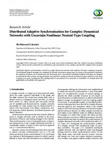
Figure 2: The state 𝑥𝑘2 and its estimate.
Let 𝑔(𝑥𝑘 ) = [sin(10𝑥𝑘 ) 0.5cos(10𝑥𝑘 )]𝑇 and set 𝑆𝑘 = 2. Let 𝜔𝑘 = 𝑒−𝑘/35 . Choose 𝑈 = 0.1, 𝑉 = 0.2, and 𝐽 = 0.25, and we solve the optimaization problem given in Theorem 9 using Matlab toolbox and obtain 𝜆 = 0.7. Set 𝛾 = 1, 𝜉0 = [0.3 0.25 0 0]𝑇 , Ξ = 𝐼, and 𝑁 = 3. Set the initial value of the system state and its estimate by 𝑥0 = [0.3 0.25]𝑇 and 𝑥̂0 = [0 0]𝑇 , and the initial values of 𝑋0 and 𝑍0 are selected to be 𝑋0 = 𝑍0 = 2𝐼. We can see the effectiveness and applicability of the proposed filtering algorithm from the simulation results (Figures 1-2).
[3] H. Gao and T. Chen, “𝐻∞ estimation for uncertain systems with limited communication capacity,” IEEE Transactions on Automatic Control, vol. 52, no. 11, pp. 2070–2084, 2007. [4] M. Sahebsara, T. Chen, and S. L. Shah, “Optimal 𝐻2 filtering in networked control systems with multiple packet dropout,” IEEE Transactions on Automatic Control, vol. 52, no. 8, pp. 1508–1513, 2007. [5] X. Lu, L. Xie, H. Zhang, and W. Wang, “Robust Kalman filtering for discrete-time systems with measurement delay,” IEEE Transactions on Circuits and Systems II: Express Briefs, vol. 54, no. 6, pp. 522–526, 2007. [6] L. Ma, Z. Wang, J. Hu, Y. Bo, and Z. Guo, “Robust varianceconstrained filtering for a class of nonlinear stochastic systems with missing measurements,” Signal Processing, vol. 90, no. 6, pp. 2060–2071, 2010. [7] L. Ma, Z. Wang, Y. Bo, and Z. Guo, “Robust 𝐻∞ sliding mode control for nonlinear stochastic systems with multiple data packet losses,” International Journal of Robust and Nonlinear Control, vol. 22, no. 5, pp. 473–491, 2012. [8] J. C. Delvenne, “An optimal quantized feedback strategy for scalar linear systems,” IEEE Transactions on Automatic Control, vol. 51, no. 2, pp. 298–303, 2006.
Discrete Dynamics in Nature and Society [9] N. Elia and S. K. Mitter, “Stabilization of linear systems with limited information,” IEEE Transactions on Automatic Control, vol. 46, no. 9, pp. 1384–1400, 2001. [10] D. Liberzon, “Hybrid feedback stabilization of systems with quantized signals,” Automatica, vol. 39, no. 9, pp. 1543–1554, 2003. [11] E. Fridman and M. Dambrine, “Control under quantization, saturation and delay: an LMI approach,” Automatica, vol. 45, no. 10, pp. 2258–2264, 2009. [12] D. Ding, Z. Wang, B. Shen, and H. Dong, “Envelopeconstrained 𝐻∞ filtering with fading measurements and randomly occurring nonlinearities: the finite horizon case,” Automatica, vol. 55, pp. 37–45, 2015. [13] B. Sinopoli, L. Schenato, M. Franceschetti, K. Poolla, M. I. Jordan, and S. S. Sastry, “Kalman filtering with intermittent observations,” IEEE Transactions on Automatic Control, vol. 49, no. 9, pp. 1453–1464, 2004. [14] R. W. Brockett and D. Liberzon, “Quantized feedback stabilization of linear systems,” IEEE Transactions on Automatic Control, vol. 45, no. 7, pp. 1279–1289, 2000. [15] H. Dong, Z. Wang, J. Lam, and H. Gao, “Distributed filtering in sensor networks with randomly occurring saturations and successive packet dropouts,” International Journal of Robust and Nonlinear Control, vol. 24, no. 12, pp. 1743–1759, 2014. [16] H. Dong, Z. Wang, and H. Gao, “Distributed 𝐻∞ filtering for a class of markovian jump nonlinear time-delay systems over lossy sensor networks,” IEEE Transactions on Industrial Electronics, vol. 60, no. 10, pp. 4665–4672, 2013. [17] H. Dong, Z. Wang, and H. Gao, “Distributed filtering for a class of time-varying systems over sensor networks with quantization errors and successive packet dropouts,” IEEE Transactions on Signal Processing, vol. 60, no. 6, pp. 3164–3173, 2012. [18] D. Ding, Z. Wang, H. Dong, and H. Shu, “Distributed 𝐻∞ state estimation with stochastic parameters and nonlinearities through sensor networks: the finite-horizon case,” Automatica, vol. 48, no. 8, pp. 1575–1585, 2012. [19] J. Liang, Z. Wang, and X. Liu, “Distributed state estimation for discrete-time sensor networks with randomly varying nonlinearities and missing measurements,” IEEE Transactions on Neural Networks, vol. 22, no. 3, pp. 486–496, 2011. [20] J. Liang, Z. Wang, and X. Liu, “Distributed state estimation for uncertain Markov-type sensor networks with mode-dependent distributed delays,” International Journal of Robust and Nonlinear Control, vol. 22, no. 3, pp. 331–346, 2012. [21] B. Shen, Z. Wang, Y. S. Hung, and G. Chesi, “Distributed 𝐻∞ filtering for polynomial nonlinear stochastic systems in sensor networks,” IEEE Transactions on Industrial Electronics, vol. 58, no. 5, pp. 1971–1979, 2011. [22] B. Shen, Z. Wang, and Y. S. Hung, “Distributed 𝐻∞ -consensus filtering in sensor networks with multiple missing measurements: the finite-horizon case,” Automatica, vol. 46, no. 10, pp. 1682–1688, 2010. [23] X. Kan, Z. Wang, and H. Shu, “State estimation for discretetime delayed neural networks with fractional uncertainties and sensor saturations,” Neurocomputing, vol. 117, pp. 64–71, 2013.
9
Advances in
Operations Research Hindawi Publishing Corporation http://www.hindawi.com
Volume 2014
Advances in
Decision Sciences Hindawi Publishing Corporation http://www.hindawi.com
Volume 2014
Journal of
Applied Mathematics
Algebra
Hindawi Publishing Corporation http://www.hindawi.com
Hindawi Publishing Corporation http://www.hindawi.com
Volume 2014
Journal of
Probability and Statistics Volume 2014
The Scientific World Journal Hindawi Publishing Corporation http://www.hindawi.com
Hindawi Publishing Corporation http://www.hindawi.com
Volume 2014
International Journal of
Differential Equations Hindawi Publishing Corporation http://www.hindawi.com
Volume 2014
Volume 2014
Submit your manuscripts at http://www.hindawi.com International Journal of
Advances in
Combinatorics Hindawi Publishing Corporation http://www.hindawi.com
Mathematical Physics Hindawi Publishing Corporation http://www.hindawi.com
Volume 2014
Journal of
Complex Analysis Hindawi Publishing Corporation http://www.hindawi.com
Volume 2014
International Journal of Mathematics and Mathematical Sciences
Mathematical Problems in Engineering
Journal of
Mathematics Hindawi Publishing Corporation http://www.hindawi.com
Volume 2014
Hindawi Publishing Corporation http://www.hindawi.com
Volume 2014
Volume 2014
Hindawi Publishing Corporation http://www.hindawi.com
Volume 2014
Discrete Mathematics
Journal of
Volume 2014
Hindawi Publishing Corporation http://www.hindawi.com
Discrete Dynamics in Nature and Society
Journal of
Function Spaces Hindawi Publishing Corporation http://www.hindawi.com
Abstract and Applied Analysis
Volume 2014
Hindawi Publishing Corporation http://www.hindawi.com
Volume 2014
Hindawi Publishing Corporation http://www.hindawi.com
Volume 2014
International Journal of
Journal of
Stochastic Analysis
Optimization
Hindawi Publishing Corporation http://www.hindawi.com
Hindawi Publishing Corporation http://www.hindawi.com
Volume 2014
Volume 2014