Hindawi Publishing Corporation Mathematical Problems in Engineering Volume 2014, Article ID 904062, 10 pages http://dx.doi.org/10.1155/2014/904062
Research Article Study of Robust 𝐻∞ Filtering Application in Loosely Coupled INS/GPS System Lin Zhao,1 Haiyang Qiu,1 and Yanming Feng2 1 2
School of Automation, Harbin Engineering University, 145 Nantong Street, Harbin 150001, China School of Electrical Engineering and Computer Science, Queensland University of Technology, 2 George Street, Brisbane, QLD 4001, Australia
Correspondence should be addressed to Haiyang Qiu;
[email protected] Received 15 April 2014; Accepted 15 May 2014; Published 4 June 2014 Academic Editor: Ligang Wu Copyright © 2014 Lin Zhao et al. This is an open access article distributed under the Creative Commons Attribution License, which permits unrestricted use, distribution, and reproduction in any medium, provided the original work is properly cited. Since a celebrate linear minimum mean square (MMS) Kalman filter in integration GPS/INS system cannot guarantee the robustness performance, a 𝐻∞ filtering with respect to polytopic uncertainty is designed. The purpose of this paper is to give an illustration of this application and a contrast with traditional Kalman filter. A game theory 𝐻∞ filter is first reviewed; next we utilize linear matrix inequalities (LMI) approach to design the robust 𝐻∞ filter. For the special INS/GPS model, unstable model case is considered. We give an explanation for Kalman filter divergence under uncertain dynamic system and simultaneously investigate the relationship between 𝐻∞ filter and Kalman filter. A loosely coupled INS/GPS simulation system is given here to verify this application. Result shows that the robust 𝐻∞ filter has a better performance when system suffers uncertainty; also it is more robust compared to the conventional Kalman filter.
1. Introduction Inertial navigation system (INS) is a self-contained system that had been widely used in military, mining, and tunnel construction in the recent decades. However, the INS parameter update functions are nonlinear, the process biases are coupled, and twice integration procedure definitely enlarges the noise influence, the dynamic error of INS keeps increasing with the time going on. Due to hardware and sensor limitation, low cost INS device can only provide an accurate navigation solution for a short period. To conquer this hardship, INS/GPS integrate system is proposed. The GPS is a time bias-free and precise system under less interference circumstance. Measurement of GPS can contribute a calibration to INS, which maintains the accuracy constant. Estimation theory is widely used in integrate navigation field that blends and fuses information to get an optimal solution. For a typical INS/GPS system, the filter dynamic equation is normally chosen by the INS error state for a linear propagation property. It calls up various investigations based on the modification of a Kalman filter to improve
the accuracy or to reduce the computation load of the system [1–3]. However, Kalman filter is the optimal estimation of minimum mean square error (MSE) for a linear time invariant (LTI) system; it has a strict requirement for the process noise covariance Q and measurement noise covariance R. If the noise is Gaussian, Kalman filter is the linear minimum variance estimator and if the noise is not Gaussian, it is linear minimum variance estimator. In practical engineering problem, we cannot absolutely assure either the statistical character of the noise or of the dynamic model. And if the objective is to achieve a minimum worst-case estimator rather than minimum variance estimator, Kalman filter will not meet the requirement. In other words, Kalman filter cannot guarantee the robustness if the system contains structure or model uncertainty and lack of noise statistical character. Motivated by this problem, precursors tried to improve the robustness performance although at the sacrifice of somewhat accuracy such as an EKF approach for parameter identification system [4]. 𝐻∞ filter is undoubtedly the best choice since it calls for no prior knowledge of the noise
2
Mathematical Problems in Engineering
distribution. Also we see application in INS/GPS area [5–7], including bounded filter theory [8], and we will review the game theory which is also called the minimax theory used in this area. It is well known that no models can all the way precisely describe a system; huge efforts have been put into the research of Robust 𝐻∞ filer. This theory assumes that there exists some uncertainty in the system and tries to solve this problem by a quadratic stabilized constrain. Riccati equation and linear matrix inequality (LMI) are two main approaches to deal with robust problems. Compared to Riccati process, LMI does not make any assumptions about the parameters and can be solved efficiently with various MATLAB toolboxes [9, 10]. 𝐻∞ theory was first applied in the control area [11]; state space realization is a bond connecting it with a estimation theory. In fact, most of research of robust 𝐻∞ filter is based on the “conservatism,” an important index in robust control. To the authors’ knowledge, there is no investigation of the robust 𝐻∞ filter considered unstable factor in INS/GPS model; here we merely discuss this application and how it can be implemented. In this paper, we firstly analyse the relationship between 𝐻∞ filter and Kalman filter and then modify the LMI design approach, making it possible to apply the robust 𝐻∞ filter for INS/GPS model; a classical 15-element (incorporating errors of attitude, velocity, position, and gyro and accelerator biases) state vector is used to check filter performance. The purpose of this paper is to make a summary and an easy access to 𝐻∞ filtering implementation in INS/GPS system. The rest of the paper is organized as follows. Derivation of recursive 𝐻∞ filter formulation based on “game theory” [12] is introduced in Section 2; in Section 3 gives designing procedure for robust 𝐻∞ filter based on LMI; Section 4 discusses the Kalman divergence issue with uncertain system and method in dealing with unstable model when using LMI; in Section 5, we compare the robust 𝐻∞ filter and Kalman filter performance in different situation for loosely coupled INS/GPS model. The notation used here is fairly standard: ‖ ⋅ ‖2 is a 𝐿 2 norm; 𝜎(𝐷) denotes the largest singular value of 𝐷; 𝑇𝑎𝑏 denotes a transform operator from 𝑎 to 𝑏; and Rn is 𝑛th dimensional Euclidian state space. Tr(𝑀) stands for the trace of matrix 𝑀, symbol ∗ represents the symmetry term in a symmetric matrix, sup means the supremum, and 𝐴𝑇 represents the transposed matrix 𝐴.
2. Game Theory Recursive 𝐻∞ Filter Since many previous authors had utilized 𝐻∞ filter in INS/GPS model, we discuss the game theory 𝐻∞ approach in this section as a fundamental illustration of the robust 𝐻∞ filter. In order to give a definition of 𝐻∞ norm. We begin with the 𝐿 2 norm. For a continuous infinite systems during the period (0, 𝑇), 𝐿 2 norm is defined as
𝑇
‖𝑥 (𝑡)‖2 = √ ∫ 𝑥 (𝑡) 𝑥𝑇 (𝑡) 𝑑𝑡, 0
(1)
where to a discrete system, suppose the sampling number is 𝑁 in the period 𝑇; then 𝑁
‖𝑥 (𝑘)‖2 = √ ∑ 𝑥 (𝑘) 𝑥𝑇 (𝑘).
(2)
𝑘=1
𝐿 2 reflects the meaning of “energy” of the variable. Then the 𝐻∞ norm of a linear, time-invariant operator 𝑔 = 𝑧(𝑤) is defined as ‖𝑧‖2 𝑇𝑔𝑤 = sup = sup 𝜎 (𝑇𝑔𝑤 (𝑗𝜔)) , (3) ∞ ‖𝑤‖2 where 𝜎(⋅) denotes the max singular value of the square matrix 𝑇 ∗ 𝑇𝑇 and 𝑗𝜔 is the frequency parameter in the range of [−𝜋, 𝜋]. In frequency domain, 𝐻∞ norm means a peak value of all the frequency ranges, while in time domain, it means the largest energy “transfer” form variable 𝑤 to variable 𝑧; in other words, 𝑤 has the largest influence on 𝑧. So what is the 𝐻∞ filter problem? Consider the following statespace system: 𝑥 (𝑘 + 1) = 𝐴𝑥 (𝑘) + 𝐵𝑤 (𝑘) , 𝑧 (𝑘) = 𝐿𝑥 (𝑘) ,
𝑦 (𝑘) = 𝐶𝑥 (𝑘) + V (𝑘) , 𝑥 (0) = 𝑥0 , (4)
where 𝑥 ∈ Rn is the dynamic state, 𝑦 ∈ Rk is the measurement, 𝑧 ∈ Rr is the output to be estimated, 𝐿𝑥(𝑡) is linear combination of 𝑥, and 𝑤 ∈ Rq and V ∈ Rp are the process and measurement noise, respectively. (𝐴, 𝐵) is controllable and (𝐴, 𝐶) is detectable. Note that it is detectable but not “observable”; in an INS/GPS model, the measurement is often “detectable” not “observable.” Now, consider such a cost function: 𝐽=
𝑧 (𝑘) − 𝑧 (𝑘)‖22𝑆𝑘 ∑𝑁 𝑘=1 ‖̂ , ̂ 2 𝑁 𝑥0 − 𝑥0 2𝑃−1 + ∑𝑘=1 (‖𝑤‖22𝑄−1 + ‖V‖22𝑅−1 ) 𝑘 𝑘 𝑘
(5)
where 𝑃𝑘 , 𝑄𝑘 , 𝑅𝑘 , and 𝑆𝑘 are symmetric, positive definite weighting matrices, and formulation ‖𝑥‖22𝑃𝑘 = 𝑥𝑃𝑘 𝑥 . Note that these weighting matrix are not noise covariance matrix in a kalman filter, they can be set arbitrary by the filter designer, of cause, can set to be equal with Kalman filter’s 𝑄, 𝑅, 𝑃. The 𝐻∞ filter problem is to find an estimation strategy 𝑧̂(𝑡) which minimizes 𝐽. The famous game theory depicted the estimation of cost function as a dynamic, two-person game: one is the engineering and the other say the nature. The goal of engineering is to find a proper estimation that minimizes 𝐽, while his opponent, the nature tries to maximize 𝐽 from the disturbances and initial state adversely. As a contrast to Kalman filter (KF), what KF pursuits is to 𝑧(𝑘) − 𝑧(𝑘)‖22𝑆𝑘 , but it cannot guarantee the 𝐽 minimize ∑𝑁 𝑘=1 ‖̂ under some fixed extent, meaning that there may be a huge noise influence on the estimation result when achieves the minimum MSE. Substituting, ‖V‖22𝑅−1 = ‖𝑦(𝑘) − 𝐶𝑥(𝑘)‖22𝑅−1 ; this problem 𝑘 𝑘 can turn to seeking a saddle point 𝐽(𝑥0∗ , 𝑤∗ , 𝑦∗ , 𝑥̂∗ ), satisfying ̂ < 𝐽 (𝑥0∗ , 𝑤∗ , 𝑦, 𝑥) ̂ < 𝐽 (𝑥0∗ , 𝑤∗ , 𝑦∗ , 𝑥̂∗ ) . (6) 𝐽 (𝑥0 , 𝑤, 𝑦, 𝑥)
Mathematical Problems in Engineering
3 So the reformed Kalman filter is given as
100
− = 𝐴 𝑘 𝑥̂𝑘− + 𝐴 𝑘 𝐾𝑘 (𝑦𝑘 − 𝐶𝑘 𝑥𝑘− ) , 𝑥̂𝑘+1
‖̂z − C1 X‖22
80
−1
𝐾𝑘 = 𝑃𝑘− (𝐼 + 𝐶𝑘𝑇 𝑅𝑘−1 𝐶𝑘 𝑃𝑘− ) 𝐶𝑘𝑇 𝑅𝑘−1 ,
60
−1
− 𝑃𝑘+1 = 𝐴 𝑘 𝑃𝑘− (𝐼 + 𝐶𝑘𝑇 𝑅𝑘−1 𝐶𝑘 𝑃𝑘− ) 𝐴𝑇𝑘 + 𝑄𝑘 .
40 20 0
Note that there is 𝑃𝑘− in (10) while 𝑃𝑘 in (11). For a LTI system, it is easy to prove that the 𝑃𝑘− and 𝑃𝑘+ converse to the same stable constant when 𝑇 → ∞, proof procedure is omitted here for brief. Now suppose that 𝛾2 = 0; the 𝐻∞ filter reduces to Kalman filter fantastically. Again, analogous to Figure 1, if the up half-surface represents the performance of the Kalman filter, this filter will pursuit the minimum MMS point, that is, ellipsoid endpoint without concerning the noise transform level. We treat the 𝐻∞ as a filter criterion, and minimax game theory provides a guarantee about this, and the noise attenuation parameter 𝛾 is also the key index in robust 𝐻∞ filter.
𝛾
−20 −40 −60 −80 −100 10
(11)
‖̂ x0 − x0 ‖22 + ‖w‖22 + ‖y − C2 X‖22 5
0
−5
−10
−10
0
−5
5
10
Figure 1: Game theory 𝐻∞ filter model.
In fact, this saddle point, that is, the smallest 𝐽, is not tractable in normal case. In general, people look for a closed form solution to the suboptimal estimation such that in Figure 1: the sole saddle point, which lies in the crossing of the upside and bottom surfaces, is difficult to achieve, while suboptimal question guarantees the solution in the range of the two planes that contains the saddle point. A summary for the game theory 𝐻∞ filter approach is: fix a prescribed parameter 𝛾 satisfying 𝐽 = 𝛾2 , 𝛾 > 0; try to 𝑧(𝑘) − 𝑧(𝑘)‖22𝑆𝑘 subject to (5). This achieve minimum ∑𝑁 𝑘=1 ‖̂ derivation process can be implemented by using the Lagrange multiplier [13, 14]. The steady-state 𝐻∞ filter formulations are given by 𝑥̂𝑘+1 = 𝐴 𝑘 𝑥̂𝑘 + 𝐴 𝑘 𝐾𝑘 (𝑦𝑘 − 𝐶𝑘 𝑥𝑘 ) , −1
𝐾𝑘 = 𝑃𝑘 (𝐼 − 𝛾2 𝑃𝑘 + 𝐶𝑘𝑇 𝑅𝑘−1 𝐶𝑘 𝑃𝑘 ) 𝐶𝑘𝑇 𝑅𝑘−1 ,
(7)
−1
𝑃𝑘+1 = 𝐴 𝑘 𝑃𝑘 (𝐼 − 𝛾2 𝑃𝑘 + 𝐶𝑘𝑇 𝑅𝑘−1 𝐶𝑘 𝑃𝑘 ) 𝐴𝑇𝑘 + 𝑄𝑘 .
−1
(8)
𝑃𝑘−
Premultiplying outside by and postmultiplying each term inside by the inverse of 𝑃𝑘− , we obtain 𝐾𝑘 =
𝑃𝑘− (𝑃𝑘−
+
−1 𝑃𝑘− 𝐶𝑘𝑇 𝑅𝑘−1 𝐶𝑘 𝑃𝑘− ) 𝑃𝑘− 𝐶𝑘𝑇 𝑅𝑘−1 .
(9)
Postmultiplying outside the parentheses by the inverse of 𝑃𝑘− and premultiplying each term inside parentheses by the inverse of 𝑃𝑘− , we have −1
𝐾𝑘 = 𝑃𝑘− (𝐼 + 𝐶𝑘𝑇 𝑅𝑘−1 𝐶𝑘 𝑃𝑘−1 ) 𝐶𝑘𝑇 𝑅𝑘−1 .
Consider a system 𝑥̇ (𝑡) = 𝐴𝑥 (𝑡) + 𝐵𝑤 (𝑡) ,
(10)
𝑦 (𝑡) = 𝐶𝑥 (𝑡) + 𝐷𝑤 (𝑡) , 𝑥 (0) = 𝑥0 .
𝑧 (𝑡) = 𝐿𝑥 (𝑡) ,
(12)
Note that the difference with system (1) lies in the description of noise. Setting 𝐵 = [𝐵 0], 𝐷 = [0 𝐷], and 𝑤 = [𝑤 V] we can get the above formula. In this term, the disturbance process and measurement noise are seen as a united element. For a system, it is impossible to obtain an exact system model due to the presence of inherent parameter uncertainty instinct. The matrices 𝐴, 𝐵, 𝐶, 𝐷 are not exactly known or depend on some time-varying parameter that vary in a fixed bound set. This is called “polytopic model” with the character 𝑆=[
For an intuitive contrast with recursive Kalman filter, some transformations are carried out here. A typical Kalman gain 𝐾𝑘 can be written as 𝐾𝑘 = (𝐼 + 𝑃𝑘− 𝐶𝑘𝑇 𝑅𝑘−1 𝐶𝑘 ) 𝑃𝑘− 𝐶𝑘𝑇 𝑅𝑘−1 .
3. Robust 𝐻∞ Filter
𝐴 𝐵 𝐴 (𝛼) 𝐵 (𝛼) ] ] ∈ {[ 𝐶 𝐷 𝐶 (𝛼) 𝐷 (𝛼) (13)
𝑁
𝐴 (𝑖) 𝐵 (𝑖) ]} = Λ. = ∑𝛼 (𝑖) [ 𝐶 (𝑖) 𝐷 (𝑖) 𝑖=1 The vector time-varying parameter 𝛼(𝑡) belongs to the unit simplex as 𝑁
Ω = {𝛼 (𝑖) ∈ 𝑅𝑛 , ∑𝛼 (𝑖) = 1; 𝛼 (𝑖) ≥ 0} .
(14)
𝑖=1
Any uncertain matrices set 𝑆(𝛼) belongs to a polytopic model with convex bound uncertain domain Λ; hence any 𝑆(𝛼) ∈ Λ, 𝑆(𝛼) can be written as a combination of vertices 𝑆(𝑖) of the convex polytope. And the model is supposed to be entirely known if the vertices number 𝑁 = 1.
4
Mathematical Problems in Engineering
Another important descriptor is the norm-bounded uncertainty. The mode 𝑆 subject to norm-bounded parameter uncertainty is written in the form 𝑆 = 𝑆0 + HFE
(15)
for the uncertain matrix parameter 𝐹 such that 𝐹𝐹 = 𝐼, 𝐻, and 𝐸 are known matrices. The purpose of the filter problem is to design an estimation 𝑧 which is given by 𝑧 = ϝ ⋅ 𝑦, where ϝ is an operator filter set with the form ̂̇ (𝑡) = 𝐴 𝑓 𝑥̂ (𝑡) + 𝐵𝑓 𝑦 (𝑡) , 𝑥
𝑧̂ (𝑡) = 𝐶𝑓 𝑥̂ (𝑡) ,
𝑥̂ (0) = 0
𝑒 (𝑡) = 𝐶𝑎 𝑥𝑖 (𝑡) ,
(17)
where 𝐴𝑎 = [
𝐴 0 ], 𝐾𝑓 𝐶 𝐴 𝑓
𝐵𝑎 = [
𝐵 ], 𝐾𝑓 𝐷
𝐶𝑎 = [𝐿 −𝐶𝑓 ] . (18)
Defining the transfer function from the noise input 𝑤 to estimation error 𝑒 is 𝑇𝑤𝑒 (𝑠); hence 𝑇𝑤𝑒 (𝑠) = 𝐶𝑎 (𝑠𝐼 − 𝐴 𝑎 )−1 𝐵𝑎 . Robust 𝐻∞ filtering problem: determining 𝐴 𝑓 , 𝐵𝑓 , 𝐶𝑓 , for all the admissible uncertainty Λ, satisfy the following: (i) model (17) is asymptotic stabilization; (ii) transfer function ‖𝑇𝑤𝑒 (𝑠)‖∞ ≤ 𝛾.
infinity
norm
holds
𝐴𝑇𝑎 𝑃𝑎 + 𝑃𝑎 𝐴 𝑎 + 𝛾−2 𝑃𝑎 𝐵𝑎 𝐵𝑎𝑇 𝑃𝑎 + 𝐶𝑎𝑇 𝐶𝑎 < 0.
that
𝐴 𝑎 𝑃 + 𝑃𝐴𝑇 𝑃𝑎 𝐶𝑎𝑇 𝐵𝑎 𝐶𝑎 𝑃𝑎 −𝛾𝐼 0 ] ] < 0. 𝑇 𝐵𝑎 0 −𝛾𝐼] [ [ [
𝐵𝑇
where ∗ denotes the symmetric block. The next step is converting this joint nonlinear matrix into LMI form [15].
(i) Solutions to LMI (20) are 𝐴 𝑎 , 𝐵𝑎 , 𝐶𝑎 , so the relationship between inequality and variables𝐴 𝑓 , 𝐵𝑓 , 𝐶𝑓 must be founded. (ii) The inequality should be transformed into linear convex optimisation problem, so it can be addressed by LMI approach. Considering the formulation (20), partition 𝑃 together with its inverse as 𝑃11 𝑃12 ], 𝑃=[ 𝑇 𝑃 𝑃 [ 12 22 ]
𝑇 𝐿𝑃11 − 𝐶𝑓 𝑃12
𝑃̂11 𝑃̂12 ], 𝑃−1 = [ ̂𝑇 𝑃̂22 𝑃 [ 12 ]
(21)
substituting the partitioned matrix 𝑃 in (17) with 𝑃11 , 𝑃22 , 𝑃̂11 , 𝑃̂22 ; the inequality changes into
𝐷𝑇 𝐵𝑓𝑇
0
∗ ] ∗ ] ], ∗ ] ] −𝛾𝐼]
(22)
Making an equivalent transform by permuting third and fourth columns and rows, we obtain
∗ ∗ 𝐴𝑃11 + 𝑃11 𝐴𝑇 [ 𝑇 𝑇 𝑇 𝑇 𝑇 𝑇 𝑇 [𝐵𝑓 𝐶𝑃11 + 𝐴 𝑓 𝑃12 + 𝑃12 𝐴 𝐵𝑓 𝐶𝑃12 + 𝐴 𝑓 𝑃22 + 𝑃12 𝐶 𝐵𝑓 + 𝑃22 𝐴 𝑓 ∗ [ [ 𝐵𝑇 𝐷𝑇 𝐵𝑓𝑇 −𝛾𝐼 [ [
(20)
3.1. LMI Approach to Robust 𝐻∞ Filtering. The LMI can be solved efficiently by the Matlab LMI Toolbox; however, two problems have to be considered.
∗ ∗ 𝐴𝑃11 + 𝑃11 𝐴𝑇 [ 𝑇 𝑇 𝑇 𝑇 𝑇 𝑇 𝑇 [𝐵𝑓 𝐶𝑃11 + 𝐴 𝑓 𝑃12 + 𝑃12 𝐴 𝐵𝑓 𝐶𝑃12 + 𝐴 𝑓 𝑃22 + 𝑃12 𝐶 𝐵𝑓 + 𝑃22 𝐴 𝑓 ∗ [ 𝑇 [ 𝐿𝑃11 − 𝐶𝑓 𝑃12 𝐿𝑃12 − 𝐶𝑓 𝑃22 −𝛾𝐼 [ [
(19)
Implement Schur complement lemma, this inequality is equivalent with the LMI:
(16)
for all the admissible uncertainty Λ such that {𝐴 𝑓 , 𝐵𝑓 , 𝐶𝑓 } ∈ ϝ. The estimation error 𝑒 can easily be yielded as 𝑒 = 𝑧 − 𝑧̂. ̂ 𝑇 , the closed loop stateConstruct state variable 𝜉 = [𝑥 𝑥] space form is 𝜉̂ (𝑡) = 𝐴 𝑎 𝜉 (𝑡) + 𝐵𝑎 𝑤 (𝑡) ;
According to the bounded real lemma, the closed loop system (17) with the upper bounded 𝛾 is asymptotically stable if and only if there exists a matrix 𝑃 = 𝑃𝑇 to such the algebraic Riccati inequality:
𝐿𝑃12 − 𝐶𝑓 𝑃22
0
∗ ] ∗ ] ]. ∗ ] ] −𝛾𝐼]
(23)
Mathematical Problems in Engineering
5
Define the nonsingular matrix −1 0 𝑃̂11 [̂ ̂ [ Ψ = [ 𝑃11 𝑃12 [ 0 0 [ 0 0
0 0 𝐼 0
0 ] 0] . ] 0] 𝐼]
(24)
Applying the congruence transformation, pre- and postmultiplying Ψ𝑇 and Ψ, the inequality can be obtained as 𝐴𝑋 + 𝑋𝐴𝑇
∗
𝐵 𝑋 𝐿−𝑍
𝐵 𝑃11 + 𝐷 𝑌 𝐿
∗
[𝐴𝑇 𝑋 + 𝑃11 𝐴 + 𝑌𝐶 + 𝐾 𝑃̂11 𝐴 + 𝐴𝑇 𝑃̂11 + 𝑌𝐶 + 𝐶𝑇 𝑌𝑇 ∗ [ 𝑇 𝑇̂ 𝑇 𝑇 [
∗ ∗
] ] > 0,
−𝛾𝐼 ∗ 0 −𝛾𝐼]
(25)
𝑌 = 𝑃̂12 ,
[
(26)
𝑋 𝑋 ] > 0. 𝑋 𝑃̂11
The objective is to determine the feasible solutions to the LMI; hence the filter matrices can be obtained: −1 −1 𝑇 𝐴𝑓 = 𝑃̂12 𝐾(𝑃12 𝑋) ,
−1 𝐵𝑓 = 𝑃̂12 𝑌,
−1
𝑇 𝐶𝑓 = 𝑍(𝑃12 𝑋) (27)
and matrices 𝑃̂12 , 𝑃12 can be set arbitrarily to be nonsingular as 𝑇 = 𝐼 − 𝑃11 𝑃̂11 . 𝑃12 𝑃̂12
(29)
−1 Define the new variable 𝑃 = 𝑃̂11 and 𝑌 = −𝐶𝑇 . Applying the Schur complement to (29), we obtain
(30)
If the parameter 𝛾 → ∞ (30) is reduced to
𝑇 𝑍 = 𝐶𝑓 𝑃12 𝑋,
𝑇 𝑋, 𝐾 = 𝑃̂12 𝐴 𝑓 𝑃12
𝑃̂11 𝐴 + 𝐴𝑇 𝑃̂11 + 𝑌𝐶 + 𝐶𝑇 𝑌𝑇 ∗ ∗ ] [ 𝑇̂ 𝑇 𝑇 [ 𝐵 𝑃11 + 𝐷 𝑌 −𝛾𝐼 ∗ ] . 𝐿 0 −𝛾𝐼] [
𝐴𝑃 + 𝑃𝐴𝑇 − 𝑃 (𝐶 𝐶 − 𝛾−2 𝐿𝑇 𝐿) 𝑃 + 𝐵𝐵𝑇 < 0.
where 𝑋, 𝑌, 𝑍, 𝐾 are matrix variables defined as −1 , 𝑋 = 𝑃11
It should be highlighted that this formulation can reduced to standard Kalman filter when restricting some special case. Suppose that 𝐵𝐷𝑇 = 0 and 𝐷𝐷𝑇 = 𝐼; a standard Kalman state description (4) can recovered from (12) when replace this strict LMI (21) by a non strict one through choosing that 𝑋 → 0, 𝐾 = −𝑌𝐶 − 𝑃̂11 𝐴, and 𝐿 = 𝑍; then the remaining variable should hold the LMI as
(28)
Here the filtering problem can be solved by a convex LMI optimisation approach. Give a summary to this filter problem. LMI 𝐻∞ filtering: minimise 𝛾 subject to inequality (26) hold. Based on the inherent properties of polytopic system, this approach can be extended to a robust filter problem. Substitute 𝐴, 𝐵, 𝐶, 𝐷 by the vertex matrices 𝐴 𝑖 , 𝐵𝑖 , 𝐶𝑖 , 𝐷𝑖 of Λ, and guaranteeing that all the vertex LMIs hold, the robust 𝐻∞ problem can be solved.
𝐴𝑃 + 𝑃𝐴𝑇 − 𝑃𝐶 𝐶𝑃 + 𝐵𝐵𝑇 < 0,
the optimal solution 𝑃 is arbitrarily close to the solution of this algebraic Riccati equation when replacing the inequality by a same equality. And this Riccati equation solution is our familiar estimation error covariance 𝑃(𝑘), when 𝑘 → ∞, also called stable state of the Kalman filter for a LTI system. 𝑇 −1 −1 and 𝑃̂12 = −𝑃̂11 and holding (28) we have Defining 𝑃11 = 𝑃12 −1
𝑇 𝐶𝑓 = 𝑍(𝑃12 𝑋)
−1
𝑇 −1 = 𝑍(𝑃12 𝑃11 )
= 𝑍 = 𝐿,
−1 −1 𝑌 = −𝑃̂11 𝑌 = 𝑃𝐶, 𝐵𝑓 = 𝑃̂12 −1
−1 𝑇 𝐴 𝑓 = 𝑃̂12 𝐾(𝑃12 𝑋)
−1 −1 = 𝑃̂12 𝐾 = 𝑃̂12 (−𝑌𝐶 − 𝑃̂11 𝐴)
(32)
−1 ̂ −1 𝑃11 ) 𝐴 − (𝑃̂12 𝑌) 𝐶 = 𝐴 − 𝐵𝑓 𝐶. = (−𝑃̂12
4. Robust 𝐻∞ to INS/GPS Loosely Coupled Model 4.1. INS Error Model. The estimation objective in GPS/INS system is the INS error. Filter for this INS dynamic error model consists of 15 elements such as
𝑥 = [𝛿𝜙𝑥 𝛿𝜙𝑦 𝛿𝜙𝑧 𝛿𝑉𝑥 𝛿𝑉𝑦 𝛿𝑉𝑧 𝛿𝐿 𝛿𝜆 𝛿ℎ 𝜀𝑥𝑏 𝜀𝑦𝑏 𝜀𝑧𝑏 ∇𝑥𝑏 ∇𝑦𝑏 ∇𝑧𝑏 ] , where 𝛿𝜙𝑥 , 𝛿𝜙𝑦 , 𝛿𝜙𝑧 are the pitch, roll, and yaw errors, 𝑉𝑥 , 𝛿𝑉𝑦 , 𝛿𝑉𝑧 are the east, north, and up velocity errors, 𝛿𝐿, 𝛿𝜆, 𝛿ℎ are the latitude, longitude, and height errors, 𝜀𝑥𝑏 , 𝜀𝑦𝑏 , 𝜀𝑧𝑏 , and ∇𝑥𝑏 , ∇𝑦𝑏 , ∇𝑧𝑏 are the gyroscope and accelerator bias errors in subscript orientation. Assume that the gyroscope and accelerator have a Gaussian white noise. The transition matrix can be written as 𝐹 (𝑡) 𝐹 (𝑡) (34) 𝐹 (𝑡) = [ 𝑁 9×9 𝑆 9×6 ] . 06×9 𝐼6×6
(31)
(33)
𝐹𝑠 (𝑡) is the 9 fundamental parameter transfer matrix of which element detailed definition can be found in [16], 𝐼 is identity matrix, and 𝐹𝑆 (𝑡) is the transfer matrix between fundamental parameter and INS sensors bias, written as 03×3 𝐶𝑏𝑛 [ 𝐹𝑆 (𝑡) = 𝐶𝑏𝑛 03×3 ] . [03×3 03×3 ]
(35)
6
Mathematical Problems in Engineering
𝐶𝑏𝑛 is the rotation matrix to transform the states from body frame to navigation frame. It is obviously that 𝐹(𝑡) is a timevarying matrix determined by the real attitude 𝜙, velocity 𝑉, and position 𝑃, although can be seen as a piecewise approximate constant matrix when implementing filtering for each epoch. 𝐻∞ estimation calls for no prestatistical character of noise, but accurate system matrices like 𝐴, 𝐵, 𝐶, 𝐷. If the INS output is corrupt, then 𝐹𝑆 cannot be guaranteed, neither is the estimation state accuracy 𝑋. And that is why a robust 𝐻∞ filter is designed for such a case. 4.2. Alternative LMI Approach to Unstable Model. It can be easy found that in a LMI approach to solve the 𝐻∞ filter context, a precondition that transfer matrix 𝐴(𝐹𝑆 ) be stable must be satisfied. The reason for this is that since the state-space model cannot be completely cancelled in the estimation error, they must be stable to guarantee the boundness of estimation error. And to apply LMI (21), it must guarantee diagonal element strictly less than 0. If 𝐴 is unstable, 𝑃 > 0, 𝐴𝑇 𝑃 + 𝑃𝐴 < 0 the first element of (21) is infeasible. To deal with this tough situation, an alternative LMI approach is proposed for coping with unstable model [17, 18]. Consider system (12), its state vector can be partitioned as 𝑥 (𝑡) = [𝑥𝑠 (𝑡) 𝑥𝑢 (𝑡)]
𝑇
(36)
and the system matrices partitions are 𝐴 (𝛼) = [
𝐵 𝐵 = [ 𝑠] , 𝐵𝑢
𝐴 𝑠 (𝛼) 0 ], 𝐴 𝑢𝑠 (𝛼) 𝐴 𝑢
𝐶 (𝛼) = [𝐶𝑠 (𝛼) 𝐶𝑢 ] ,
where 𝐴 𝑠 (𝛼) 0 0 𝐴 𝑓𝑠 −𝐴 𝑓1 ] , 𝐴 𝑎 (𝛼) = [ 𝐵𝑓𝑠 𝐶𝑠 (𝛼) [𝐴 𝑢𝑠 − 𝐵𝑓𝑢 𝐶𝑠 (𝛼) −𝐴 𝑓2 𝐴 𝑓𝑢 ] 0 𝐴 𝑎𝑢 = [ 𝐴 𝑓1 + 𝐵𝑓𝑠 𝐶𝑢 ] , [𝐴 𝑢 − 𝐵𝑓𝑢 𝐶𝑢 − 𝐴 𝑓𝑢 ] 𝐶𝑎 (𝛼) = [𝐿 𝑠 −𝐶𝑓𝑠 𝐶𝑓𝑢 ] ,
(41) So the partial state 𝑥𝑠 is bounded while 𝑥𝑢 is unbounded. If 𝜉(𝑡) and 𝑒(𝑡) are bounded, there must be assured that 𝐴 𝑎𝑢 = 0 and 𝐶𝑎𝑢 = 0, also meaning that 𝐴 𝑓1 = −𝐵𝑓𝑠 𝐶𝑢 ,
𝐿 = [𝐿 𝑠 (𝛼) 𝐿 𝑢 ] ,
(ii) The matrix 𝐴 𝑢 is unstable.
𝑥̂ (𝑘 + 1) = (𝐴 − 𝐾𝐶) 𝑥̂ (𝑡) + 𝐾𝑦 (𝑡) . 𝑥̃ (𝑘 + 1) = (𝐴 − 𝐾𝐶) 𝑥̃ (𝑘 + 1) + 𝑤 (𝑡) + 𝐾V (𝑡) .
= 𝐴 𝑥 (𝑘) − 𝐴𝑥̂ (𝑘) + 𝐾𝐶𝑥̂ (𝑘) − 𝐾𝑦 (𝑘) + 𝑤 (𝑘) = (𝐴 − 𝐴) 𝑥 (𝑘) + 𝐴 (𝑥 (𝑘) − 𝑥̂ (𝑘)) + 𝐾𝐶 (𝑥̂ (𝑘) − 𝑥 (𝑘)) − 𝐾V (𝑘) + 𝑤 (𝑘)
(38)
= (𝐴 − 𝐴) 𝑥 (𝑘) + (𝐴 − 𝐾𝐶) 𝑥̃ (𝑘)
𝐶𝑓 = [𝐶𝑓𝑠 𝐶𝑓𝑢 ] .
+ 𝑤 (𝑘) − 𝐾V (𝑘) .
Change the variable 𝜉 with a augmented state, 𝜉 will become 𝜉 = [𝑥𝑠 𝑥̂𝑥 (𝑥𝑢 − 𝑥̂𝑢 )] .
(39)
Equation (17) is reformed as 𝜉 ̇ (𝑡) = 𝐴 𝑎 (𝛼) 𝜉 (𝑡) + 𝐴 𝑎𝑢 𝑥𝑢 (𝑡) + 𝐵𝑎 𝑤 (𝑡) , 𝑒 (𝑡) = 𝐶𝑎 (𝛼) 𝜉 (𝑡) + 𝐶𝑎𝑢 𝑥𝑢 (𝑡) ,
(44)
If (𝐴−𝐾𝐶) is stable, then error dynamic function is stable, meaning KF is stable. Now, suppose that 𝐴 is uncertain, and the real matrix is 𝐴 , and 𝐴 is the nominal matrix in filtering. We obtain
Next, partition the filter matrices, and we obtain
𝐵𝑓 = [𝐵𝑓𝑠 𝐵𝑓𝑢 ] ,
(43)
𝑥̃ (𝑘 + 1) = 𝑥 (𝑘 + 1) − 𝑥̂ (𝑘 + 1)
(iii) (𝐶𝑠 , 𝐴 𝑠 ) is detectable and (𝐴, 𝐵) is controllable.
𝐴 𝑓𝑠 𝐴 𝑓1 ], 𝐴 𝑓2 𝐴 𝑓𝑢
𝐶𝑓𝑢 = 𝐿 𝑢 . (42)
The estimation error dynamic function is
(i) The subsystem 𝑥𝑠̇ (𝑡) = 𝐴 𝑠 𝑥𝑠 (𝑡) is quadratically stable.
𝐴𝑓 = [
𝐴 𝑓𝑢 = 𝐴 𝑢 − 𝐵𝑓𝑢 𝐶𝑢 ,
Now, we have solved the unstable problems and the remaining processor can use a typical LMI approach to the robust 𝐻∞ filtering. Since we cannot remove the unstable part from an entire system, the only choice is to try a decomposition of the stable and unstable parts; the key factor lies in eliminating the unbounded estimation influence rendering that the final result is not corrupted.
(37)
Assumption. Consider the following.
𝑥̂𝑠 (𝑡) ], 𝑥̂𝑢 (𝑡)
𝐶𝑎𝑢 = [𝐿 𝑢 − 𝐶𝑓𝑢 ] .
4.3. Uncertainty to Kalman Filter Divergency Issue. Another drawback when applying Kalman filter to an uncertain and unstable system is divergency issue. The steady state of (4) is
where the subscript “𝑠” denotes the stable component and “𝑢” denotes the unstable component.
𝑥̂ (𝑡) = [
𝐵𝑠 𝐵𝑎 = [ 𝐵𝑓𝑠 𝐷 ] , [𝐵𝑢 − 𝐵𝑓𝑢 𝐷]
(45) The above formulation can be written as [
(40)
𝐴 0 𝑥 (𝑘 + 1) 𝑥 (𝑘) ]= [ ][ ] 𝑥̃ (𝑘 + 1) 𝐴 − 𝐴 𝐴 − 𝐾𝐶 𝑥̃ (𝑘) 𝑤 (𝑘) +[ ]. 𝑤 (𝑘) − 𝐾V (𝑘)
(46)
Mathematical Problems in Engineering
7 1
1000
0
150
0
𝛿P (m)
𝛿V (m/s)
𝜙 (arcmin)
200
0.5
500
−0.5
−500
−1000
250
50
−1
0
200
400
−1.5
600
100
0 0
200
400
t (s)
−50
600
0
200
1
400
600
t (s)
t (s) 1500 1000
0 ∇ (𝜇g)
𝜀 (∘ /h)
500 −1
0 −500
−2 −1000 −3
0
200
400
−1500
600
0
200
0.8
0
0.6
−0.05
0.4
−0.1
250 200 150
0.2
0
200
400
−0.2
600
0 0
200
t (s)
400
600
−50
0
t (s)
0.01
100.6
∇ (𝜇g)
0.01 0.01 0.01
100.4 100.2 100
0.01 0
200
400 t (s)
600
0
200
200
400 t (s)
100.8
0.01
𝜀 (∘ /h)
100 50
0
−0.15
0.01
600
𝛿P (m)
0.05
−0.2
400 t (s)
𝛿V (m/s)
𝜙 (arcmin)
t (s)
400
600
t (s)
Figure 2: Normal situation Kalman filter and robust 𝐻∞ filter results.
600
8
Mathematical Problems in Engineering 1000
1
0
−500
150
0
𝛿P (m)
𝛿V (m/s)
𝜙 (arcmin)
200
0.5
500
−1000
250
−0.5
50
−1
0
200
400
−1.5
600
100
0 0
200
t (s)
400
−50
600
0
200
4
400
600
400
600
t (s)
t (s) 2000
3 1000 ∇ (𝜇g)
𝜀 (∘ /h)
2 1
0
0 −1000 −1 −2
0
200
400
−2000
600
0
200
600
0.8
0.1
0.6
0
0.4
−0.1 −0.2
250 200 150 𝛿P (m)
0.2
−0.3
400 t (s)
𝛿V (m/s)
𝜙 (arcmin)
t (s)
0.2
50
0
0
200
400
−0.2
600
0 0
200
t (s)
×10−3 10.04
100
400
600
−50
0
t (s)
t (s)
101
10.02
∇ (𝜇g)
𝜀 (∘ /h)
100.5 10 9.98
100
9.96 9.94
0
200
400 t (s)
600
99.5
0
200
200
400
600
t (s)
Figure 3: Interfered situation Kalman filter and robust 𝐻∞ filter results.
Mathematical Problems in Engineering
9
5
5
0 −5
0
500
1000
0 −5
1500
×109 1
𝛿P (m)
×108 10 𝛿V (m/s)
𝜙 (arcmin)
Kalman filter estimation error ×109 10
0
500
t (s)
0
500
0
0
−0.5
500
1000
Robust H∞ filter estimation error
0
500
t (s)
1000
1000
1500
500 0 −500
0
500
t (s) North East
Pitch Roll Yaw
1500
North East
−2 −4
1500
1000 t (s)
𝛿P (m)
2 𝛿V (m/s)
𝜙 (arcmin)
−2
1500
North East
0.5
0
−1
t (s)
Pitch Roll Yaw
−1
1000
0
1000
1500
t (s) North East
Figure 4: Normal situation Kalman filter and robust 𝐻∞ filter results for 1500 s.
If 𝐴 and 𝐴 are both unstable, when 𝑘 → ∞, 𝑥(𝑡) can be ̃ can be arbitrarily large, so even 𝐴 − 𝐴 is small; hence 𝑥(𝑘) arbitrarily large, and the filer is divergent.
5. Simulation Result The state model is as (34), observations are the difference between INS and GPS position measurement. This simulation chooses a static condition, and its period lasts for 500 s. Gyros constant drift and random white noise 1 sigma are 0.02∘ /h and 0.01∘ /h; accelerator constant drift and random white noise 1 sigma are 100 𝜇g and 10 𝜇g. GPS position measurement white noise 1 sigma is 1 m/s. Corresponding correlation noise matrices are set as 𝑄 = diag (06×1 ; [0.01 m, 0.01 m, 0.01 m] ; [0.01∘ /h, 0.01∘ /h, 0.01∘ /h] ; 2
[10 𝜇g, 10 𝜇g, 10 𝜇g]) ,
(47)
𝑅 = diag ([1 m, 1 m, 1 m])2 . Initial estimation error correlation matrix can be given as 𝑃 = diag ([1∘ , 1∘ , 1∘ ] , [1 m/s, 1 m/s, 1 m/s] , [10 m, 10 m, 10 m] , [0.1∘ /h, 0.1∘ /h, 0.1∘ /h] , [100 𝜇g, 100 𝜇g, 100 𝜇g]) . (48)
This simulation software details can be found in [19], since compared to INS, GPS measurement is more easily interfered; two scenarios are considered. (i) Normal situation means that there is an accurate prior information for the noise character. (ii) Interfered situation means that the GPS measurement noise is 5 times compared to nominal noise character during 100–200 s. Results are shown in Figures 2 and 3; pink curve represents the real value. Subpictures show the error attitude, error velocity, error position, gyro bias, and accelerator bias in turn. Because the up direction is divergent, only north and east results are shown here. Triple INS compensate parameters 𝛿𝜙, 𝛿𝑉, 𝛿𝑃 statistical index STD is shown in Tables 1 and 2 for these two situations. In normal situation, KF shows a more “stable” and “accurate” performance than 𝐻∞ filter; the 𝐻∞ filter exhibits a jitter character in the tracking process of real value, whereas in interfered situation, 𝐻∞ filter is more robust, takes account of the north 𝛿𝑉, 𝐻∞ filter STD varies from 0.0366 to 0.0372 while KF from 0.0296 to 0.0473. Note that 𝐻∞ filter contributes a better performance to 𝛿𝜙 in both situations because 𝐻∞ filter has a “weak” effect on estimation error matrix 𝑃 which means that the initial value 𝑃 has a weak influence. In the follow scenario, we extend the simulation time to 1500 s without calibration to INS using the filter output, result is shown in Figure 4. The Kalman filter suffers a
10
Mathematical Problems in Engineering Table 1: Normal situation STD index.
STD
Pitch 𝜙𝑜 0.1130 North 𝛿𝑉 m/s 0.0296 𝛿𝑃 m 0.2806
Kalman Roll 0.1386 East 0.0266 0.3487
Yaw 2.4796 Up Nan Nan
Pitch 0.0129 North 0.0366 0.6351
Robust 𝐻∞ Roll Yaw 0.0149 0.035 East Up 0.0519 Nan 0.8284 Nan
Table 2: Interfered situation STD index. STD 𝜙𝑜 𝛿𝑉 m/s 𝛿𝑃 m
Pitch 0.1430 North 0.0473 0.4206
Kalman Roll 0.1786 East 0.0565 0.5787
Yaw 2.9196 Up Nan Nan
Pitch 0.0159 North 0.0372 0.8321
Robust 𝐻∞ Roll Yaw 0.0199 0.055 East Up 0.0568 Nan 0.9674 Nan
divergence. Although there is a large trend of the estimation error, 𝐻∞ is stable during this period.
6. Conclusion In this paper, we design a robust 𝐻∞ filter for a loosely coupled INS/GPS model. Firstly, a game theory gives a 𝐻∞ approach in a Kalman form; it can be easily transformed by adjusting the noise attenuation parameter 𝛾. Next, a robust 𝐻∞ filter based LMI is discussed; the unstable case is considered. We also illustrate that the robust 𝐻∞ filter based on LMI approach can convert into standard KF in special conditions. For a direct performance contrast, simulation result shows the INS error estimate state that is not compensated for INS. This proposed approach may be applied in a system under uncertainty such as low-cost IMU and interfered GPS environment.
Conflict of Interests The authors declare that there is no conflict of interests regarding the publication of this paper.
Acknowledgments This research was funded by the State Scholarship Fund of the China Scholarships Council (CSC). The authors would like to thank all the editors and anonymous reviewers for improving this paper.
References [1] J. Ali and F. Jiancheng, “SINS/ANS/GPS integration using federated kalman filter based on optimized information-sharing coefficients,” in Proceedings of the AIAA Guidance, Navigation, and Control Conference, pp. 1–13, August 2005. [2] E. J. Lefferts, F. L. Markley, and M. D. Shuster, “Kalman filtering for spacecraft attitude estimation,” Journal of Guidance, Control, and Dynamics, vol. 5, no. 5, pp. 417–429, 1982.
[3] A. H. Mohamed and K. P. Schwarz, “Adaptive Kalman filtering for INS/GPS,” Journal of Geodesy, vol. 73, no. 4, pp. 193–203, 1999. [4] G. Sun, M. Wang, and L. Wu, “Unexpected results of extended fractional kalman filter for parameter identification in fractional order chaotic systems,” International Journal of Innovative Computing, Information and Control, vol. 7, no. 9, pp. 5341–5352, 2011. [5] X. F. He, Y. Q. Chen, and B. Vik, “Design of minimax robust filtering for an integrated GPS/INS system,” Journal of Geodesy, vol. 73, no. 8, pp. 407–411, 1999. [6] X.-K. Yue and J.-P. Yuan, “𝐻∞ sub-optimal filter for low-cost integrated navigation system,” Chinese Journal of Aeronautics, vol. 17, no. 4, pp. 200–206, 2004. [7] N. Abdelkrim, N. Aouf, A. Tsourdos, and B. White, “Robust nonlinear filtering for INS/GPS UAV localization,” in Proceedings of the Mediterranean Conference on Control and Automation (MED ’08), pp. 695–702, June 2008. [8] G. A. Einicke, G. Falco, and J. T. Malos, “Bounded constrained filtering for GPS/INS integration,” IEEE Transactions on Automatic Control, vol. 58, no. 1, pp. 125–133, 2013. [9] J. L¨ofberg, “YALMIP: a toolbox for modeling and optimization in MATLAB,” in Proceedings of the IEEE International Symposium on Computer Aided Control System Design, pp. 284–289, September 2004. [10] P. Gahinet, A. Nemirovskii, A. J. Laub, and M. Chilali, “LMI control toolbox,” in Proceedings of the 2nd IEEE International Symposium on Requirements Engineering, pp. 2038–2041, March 1994. [11] L. Wu, J. Lam, W. Paszke, K. Gałkowski, E. Rogers, and A. Kummert, “Control and filtering for discrete linear repetitive processes with 𝐻∞ and 𝑙2 − 𝑙∞ performance,” Multidimensional Systems and Signal Processing, vol. 20, no. 3, pp. 235–264, 2009. [12] U. Shaked and Y. Theodor, “H-optimal estimation: a tutorial,” in Proceedings of the 31st IEEE Conference on Decision and Control, pp. 2278–2286, 1992. [13] D. Simon, Optimal State Estimation: Kalman, H Infinity, and Nonlinear Approaches, Wiley-Interscience, 2009. [14] X. Shen and L. Deng, “Game theory approach to discrete 𝐻∞ filter design,” IEEE Transactions on Signal Processing, vol. 45, no. 4, pp. 1092–1095, 1997. [15] S. H. Jin and J. B. Park, “Robust 𝐻∞ filtering for polytopic uncertain systems via convex optimisation,” IEE Proceedings: Control Theory and Applications, vol. 148, no. 1, pp. 55–59, 2001. [16] A. Noureldin, T. B. Karamat, M. D. Eberts, and A. El-Shafie, “Performance enhancement of MEMS-based INS/GPS integration for low-cost navigation applications,” IEEE Transactions on Vehicular Technology, vol. 58, no. 3, pp. 1077–1096, 2009. [17] L. Xie, C. E. de Souza, and Y. C. Soh, “Robust filtering for uncertain systems with unstable modes,” in Proceedings of the 33rd IEEE Conference on Decision and Control, pp. 3929–3930, December 1994. [18] K. Barbosa, C. E. de Souza, and A. Trofino, “Robust 𝐻∞ filtering for uncertain linear systems with unstable modes,” in Proceedings of the IFAC Symposium on System, Structure and Control, vol. 4, pp. 253–258, 2004. [19] Y. Gomgmin, “Strapdown inertial navigation simulation toolbox in matlab,” Northwestern Polytechnical University of China, 2013, http://blog.sina.com.cn/u/1089338825.
Advances in
Operations Research Hindawi Publishing Corporation http://www.hindawi.com
Volume 2014
Advances in
Decision Sciences Hindawi Publishing Corporation http://www.hindawi.com
Volume 2014
Journal of
Applied Mathematics
Algebra
Hindawi Publishing Corporation http://www.hindawi.com
Hindawi Publishing Corporation http://www.hindawi.com
Volume 2014
Journal of
Probability and Statistics Volume 2014
The Scientific World Journal Hindawi Publishing Corporation http://www.hindawi.com
Hindawi Publishing Corporation http://www.hindawi.com
Volume 2014
International Journal of
Differential Equations Hindawi Publishing Corporation http://www.hindawi.com
Volume 2014
Volume 2014
Submit your manuscripts at http://www.hindawi.com International Journal of
Advances in
Combinatorics Hindawi Publishing Corporation http://www.hindawi.com
Mathematical Physics Hindawi Publishing Corporation http://www.hindawi.com
Volume 2014
Journal of
Complex Analysis Hindawi Publishing Corporation http://www.hindawi.com
Volume 2014
International Journal of Mathematics and Mathematical Sciences
Mathematical Problems in Engineering
Journal of
Mathematics Hindawi Publishing Corporation http://www.hindawi.com
Volume 2014
Hindawi Publishing Corporation http://www.hindawi.com
Volume 2014
Volume 2014
Hindawi Publishing Corporation http://www.hindawi.com
Volume 2014
Discrete Mathematics
Journal of
Volume 2014
Hindawi Publishing Corporation http://www.hindawi.com
Discrete Dynamics in Nature and Society
Journal of
Function Spaces Hindawi Publishing Corporation http://www.hindawi.com
Abstract and Applied Analysis
Volume 2014
Hindawi Publishing Corporation http://www.hindawi.com
Volume 2014
Hindawi Publishing Corporation http://www.hindawi.com
Volume 2014
International Journal of
Journal of
Stochastic Analysis
Optimization
Hindawi Publishing Corporation http://www.hindawi.com
Hindawi Publishing Corporation http://www.hindawi.com
Volume 2014
Volume 2014