Hindawi Publishing Corporation Mathematical Problems in Engineering Volume 2015, Article ID 869482, 14 pages http://dx.doi.org/10.1155/2015/869482
Research Article Strong Tracking Filtering Algorithm of Randomly Delayed Measurements for Nonlinear Systems Hongtao Yang,1,2,3 Huibin Gao,1 and Xin Liu1 1
Changchun Institute of Optics, Fine Mechanics and Physics, Chinese Academy of Sciences, Changchun 130033, China University of Chinese Academy of Sciences, Beijing 100049, China 3 College of Electrical and Electronic Engineering, Changchun University of Technology, Changchun 130012, China 2
Correspondence should be addressed to Hongtao Yang; hongtao
[email protected] Received 17 June 2015; Revised 23 September 2015; Accepted 28 September 2015 Academic Editor: Asier Ibeas Copyright © 2015 Hongtao Yang et al. This is an open access article distributed under the Creative Commons Attribution License, which permits unrestricted use, distribution, and reproduction in any medium, provided the original work is properly cited. This paper focuses on the filtering problems of nonlinear discrete-time stochastic dynamic systems, such as the model simplification, noise characteristics uncertainty, initial conditions uncertainty, or system parametric variation. Under these circumstances, the measurements of system have one sampling time random delay. A new method, that is, strong tracking filtering algorithm of randomly delayed measurements (STF/RDM) for nonlinear systems based on recursive operating by analytical computation and first-order linear approximations, is proposed; a principle of extended orthogonality is presented as a criterion of designing the STF/RDM, and through the residuals between available and predicted measurements, the formula of fading factor is obtained. Under the premise of using the extended orthogonality principle, STF/RDM proposed in this paper can adjust the fading factor online via calculating the covariance of residuals, and then the gain matrices of the STF/RDM adjust in real time to enhance the performance of the proposed method. Lastly, in order to prove that the performance of STF/RDM precedes existing EKF method, the experiment of tracking maneuvering aircraft is carried out.
1. Introduction Filtering task is obtaining state variables from a series of noisy measurements available online. The main aim is to minimize the estimation error, which is referred to as the residual or innovation vector. Currently, most suboptimal methods for obtaining the posterior density in nonlinear discrete-time stochastic dynamic systems are using global and local approximation methods. Taking the point-mass filter based on adaptive algorithm [1] and particle filters with Gaussian mixtures based on Gaussian mixture approximation [2], for example, it is the advantage of the global approximate approach that any clear assumption pertaining to the form of posterior density is not needed. Although the global methods have strong adaptability, they suffer from enormous computational complexity. In contrast, the local methods have simple design of the filter and fast implementing speed, and the performance of this method is always with acceptable accuracy in actual applications. In local methods, the form of posterior density usually
is assumed to be Gaussian. Sometimes several local filters can be derived without an assumption on the density (just the first two moments are required) such as extended Kalman filter or unscented Kalman filter. Up till now, there are plenty of variations about local methods of approximation, such as the extended Kalman filter (EKF) based on the method of linearization [3], the central-difference Kalman filter (CDKF) based on the interpolation method [4], the unscented Kalman filter (UKF) based on the method of unscented transform [5], the quadrature Kalman filter (QKF) based on the rule of Gauss-Hermite [6], and the cubature Kalman filter (CKF) based on the cubature rule of spherical-radial cubature [7]. However, since the aforementioned state estimation methods are all formulated under the assumption of statistics of the noises and system parameters accurate modeling, in real applications they have some disadvantages; for example, the uncertainties in the model, initial conditions, or noise characteristics may lead to bias in the estimation process. In order to overcome the above disadvantages, one solution is to introduce fading factors in the state error covariance matrix based
2 on the residual sequence. This method is named as the strong tracking filter (STF), which was proposed by Zhou and Frank [8–11]. In general, all the above filtering estimations often consider the fact that in real time the measurements generated by system are available, but the measurements directly obtained are affected by random delay in many actual applications. Therefore, the problem of filtering having randomly delayed measurements has been attracting wide attention [12–15], in nonlinear state estimation. In [12], two modified filtering algorithms, EKF and UKF, with one sampling time randomly delayed measurements have been proposed; an improved unscented filtering algorithm in [13] was proposed based on two-step randomly delayed measurements; the literature [14] considered one-stage prediction, filtering, and fixed-point smoothing problems in nonlinear discrete-time stochastic systems having one-step randomly delayed measurements; in this situation, the recursive estimation algorithm, that is, the signal produced by state-space model is uncertain and only the covariance information can be utilized, has been proposed; recently, considering observations of one-step randomly delayed measurements, a generic framework of Gaussian approximation (GA) filter has been given in [15]. To overcome the common disadvantages of filtering method having one-step randomly delayed measurements and normal filtering method, here, a novel STF/RDM is proposed; an extended orthogonality principle is presented as a criterion of designing the STF/RDM and through the residuals between available and predicted measurements, the formula of fading factor is obtained. Since the STF/RDM can implement the online tuning of the fading factor by monitoring the covariance of residuals, the gain of the STF/RDM will be adjusted in real time to enhance performance of ESFT. The structure of this paper is as follows. The basis of theory and elementary knowledge about the existing EKF having one-step randomly delayed measurements is reviewed in Section 2. Then, the extended orthogonality principle which is the basis of STF/RDM is proposed in Section 3. Thereafter, in Section 4, the STF/RDM having one-step randomly delayed measurements is derived. In Section 5, simulation experiment on tracking a maneuvering aircraft is implemented to compare the performance of the STF/RDM with existing EKF. Finally, Section 6 gives some conclusions. Throughout this paper, 𝐸[⋅] stands for mathematical expectation; 𝐼 stands for the unit matrix; diag{⋅ ⋅ ⋅ } denotes a block-diagonal matrix; the superscripts −1, 𝑇, ∧ , and ∼, respectively, denote the inverse matrix, the matrix transposition, the estimate, and the estimation error. For example, 𝑥̂ stands for the estimate of variable 𝑥 and 𝑥̃ = 𝑥 − 𝑥̂ stands for the estimate error of variable 𝑥.
2. Problem Formulation and Preliminaries In this section, the nonlinear model having one-step randomly delayed observations and the filtering algorithm derived from this model are reviewed.
Mathematical Problems in Engineering 2.1. Nonlinear System Model. Consider a nonlinear, discretetime, stochastic system as state model shown by 𝑥𝑘+1 = 𝑓𝑘 (𝑥𝑘 ) + 𝑤𝑘 ,
𝑘≥0
(1)
and the model of one sampling randomly delayed observation 𝑧𝑘 = ℎ𝑘 (𝑥𝑘 ) + V𝑘 ,
𝑘 ≥ 1,
𝑦𝑘 = (1 − 𝛾𝑘 ) 𝑧𝑘 + 𝛾𝑘 𝑧𝑘−1 ,
(2) 𝑘 > 1; 𝑦1 = 𝑧1 ,
(3)
where {𝑥𝑘 ; 𝑘 ≥ 0} is the 𝑛 × 1 state vector, {𝑧𝑘 ; 𝑘 ≥ 1} is the 𝑚 × 1 real measurement, {𝑦𝑘 ; 𝑘 > 1} is the 𝑚 × 1 available measurements, {𝑤𝑘 ; 𝑘 ≥ 0} and {V𝑘 ; 𝑘 ≥ 1} are sequences of uncorrelated Gaussian white noises that have zero means and the covariance matrices which are 𝐸[𝑤𝑘 𝑤𝑙𝑇 ] = 𝑄𝑘 𝛿𝑘𝑙 and 𝐸[V𝑘 V𝑙𝑇 ] = 𝑅𝑘 𝛿𝑘𝑙 , respectively, where 𝛿𝑘𝑙 is the Kronecker delta function, the initial state 𝑥0 is a random Gaussian vector having mean 𝐸[𝑥0 ] = 𝑥̂0|0 and covariance 𝐸[𝑥0 𝑥0𝑇 ] = 𝑃0|0 , for all 𝑘, the nonlinear functions 𝑓𝑘 and ℎ𝑘 are infinitely continuously differentiable, and {𝛾𝑘 ; 𝑘 > 1} denotes a sequence of uncorrelated Bernoulli random variables that can take the values 0 or 1 with 𝑝 (𝛾𝑘 = 1) = 𝐸 [𝛾𝑘 ] = 𝑝𝑘 , 𝑝 (𝛾𝑘 = 0) = 1 − 𝐸 [𝛾𝑘 ] = 1 − 𝑝𝑘 , 2
𝐸 [(𝛾𝑘 − 𝑝𝑘 ) ] = (1 − 𝑝𝑘 ) 𝑝𝑘 ,
(4)
𝐸 [(𝛾𝑘 − 𝑝𝑘 )] = 0, where 𝑝𝑘 represents the probability of a delay in measurement at time 𝑘. Substituting (2) into (3) gives 𝑦𝑘+1 = (1 − 𝛾𝑘 ) [ℎ𝑘+1 (𝑥𝑘+1 ) + V𝑘+1 ] + 𝛾𝑘+1 [ℎ𝑘 (𝑥𝑘 ) + V𝑘 ] .
(5)
In (1)–(3), assume that 𝑥0 , {𝑤𝑘 ; 𝑘 ≥ 0}, {V𝑘 ; 𝑘 ≥ 1}, and {𝛾𝑘 ; 𝑘 > 1} are mutually independent. Obviously, the Bernoulli variable in (3) imitates the random delay in the following sense: at each time 𝑘 > 1, if 𝛾𝑘 = 1, then 𝑦𝑘 = 𝑧𝑘−1 which means that the measurement is one sampling time randomly delayed; otherwise, if 𝛾𝑘 = 0, then 𝑦𝑘 = 𝑧𝑘 which means that the measurement is updated. 2.2. Extended Kalman Filter with One-Step Randomly Delayed Observations. In [15], a general and common framework of Gaussian approximation (GA) applied in the system shown by (1)–(3) has been presented; under these circumstances, the measurements with one sampling time random delay often occur. Here, the functions of one-step posterior predictive probability density 𝑝(𝑥𝑘+1 | 𝑌𝑘 ) and 𝑝(𝑦𝑘+1 | 𝑌𝑘 ) are all assumed to be Gaussian, where 𝑌𝑘 = {𝑦𝑖 }𝑘𝑖=1 is the set of the available measurements in (3). In (5), it is clear that the Gaussian approximation of 𝑝(𝑥𝑘+1 | 𝑌𝑘+1 ) and 𝑝(V𝑘+1 | 𝑌𝑘+1 ) needs to be known when deriving a GA filter for the system
Mathematical Problems in Engineering
3
in (1)–(3). Therefore, the augmented state vector is defined as follows: 𝑎 =( 𝑥𝑘+1
𝑥𝑘+1 V𝑘+1
),
(6)
whose mean and covariance are conditioned by 𝑌𝑘+1 , approximated by 𝑎 =( 𝑥̂𝑘+1|𝑘+1
𝑎 𝑃𝑘+1|𝑘+1
𝑥̂𝑘+1|𝑘+1 ̂V𝑘+1|𝑘+1
=(
), 𝑥V 𝑃𝑘+1|𝑘+1
𝑃𝑘+1|𝑘+1 𝑥V (𝑃𝑘+1|𝑘+1 )
𝑇
VV 𝑃𝑘+1|𝑘+1
(7) ).
Note that V𝑘+1 is independent of 𝑌𝑘 and 𝑥̃𝑘+1|𝑘 . Hence, the 𝑎 𝑎 and the covariance 𝑃𝑘+1|𝑘 augmented state prediction 𝑥̂𝑘+1|𝑘 are 𝑥̂𝑘+1|𝑘 𝑎 𝑥̂𝑘+1|𝑘 =( ), 0𝑚×1
(8)
𝑃𝑘+1|𝑘 0𝑛×𝑚 𝑎 =( ). 𝑃𝑘+1|𝑘 0𝑚×𝑛 𝑅𝑘+1
In [15], the equations describing the Gaussian approximation (GA) filter applied in the system shown by (1)–(3) are as follows: 𝑥 𝑥̂𝑘+1|𝑘+1 = 𝑥̂𝑘+1|𝑘 + 𝐾𝑘+1 𝑦̃𝑘+1|𝑘 ,
(9)
V ̂V𝑘+1|𝑘+1 = 𝐾𝑘+1 𝑦̃𝑘+1|𝑘 ,
(10) 𝑇
𝑦𝑦
𝑥 𝑥 𝑃𝑘+1|𝑘+1 = 𝑃𝑘+1|𝑘 − 𝐾𝑘+1 𝑃𝑘+1|𝑘 (𝐾𝑘+1 ) ,
(11)
𝑇
𝑦𝑦
𝑥V 𝑥 V 𝑃𝑘+1|𝑘+1 = −𝐾𝑘+1 𝑃𝑘+1|𝑘 (𝐾𝑘+1 ) , 𝑦𝑦
(12) 𝑇
VV V V 𝑃𝑘+1|𝑘+1 = 𝑅𝑘+1 − 𝐾𝑘+1 𝑃𝑘+1|𝑘 (𝐾𝑘+1 ) , 𝑥𝑦
𝑦𝑦
(13)
−1
𝑥 = 𝑃𝑘+1|𝑘 (𝑃𝑘+1|𝑘 ) , 𝐾𝑘+1
(14)
𝑥𝑘+1 ≈ 𝑓𝑘 (𝑥̂𝑘|𝑘 ) + 𝐹𝑘 (𝑥𝑘 − 𝑥̂𝑘|𝑘 ) + 𝑤𝑘 ,
(20)
𝑧𝑘 ≈ ℎ𝑘 (𝑥̂𝑘|𝑘 ) + 𝐻𝑘 (𝑥𝑘 − 𝑥̂𝑘|𝑘 ) + V𝑘 ,
(21)
where 𝐹𝑘 = 𝜕𝑓𝑘 (𝑥𝑘 )/𝜕𝑥𝑘 |𝑥𝑘 =𝑥̂𝑘|𝑘 and 𝐻𝑘 = 𝜕ℎ𝑘 (𝑥𝑘 )/𝜕𝑥𝑘 |𝑥𝑘 =𝑥̂𝑘|𝑘 . Then, 𝑥̂𝑘+1|𝑘 and 𝑃𝑘+1|𝑘 are approximated by the linear Kalman filter: 𝑥̂𝑘+1|𝑘 = 𝑓𝑘 (𝑥̂𝑘|𝑘 ) ,
(22)
𝑃𝑘+1|𝑘 = 𝐹𝑘 𝑃𝑘|𝑘 𝐹𝑘𝑇 + 𝑄𝑘 .
(23)
Moreover, given 𝑥̂𝑘+1|𝑘 and 𝑃𝑘+1|𝑘 by (22) and (23), by linearization of ℎ𝑘+1 (𝑥𝑘+1 ) with the first term of the Taylor series expansion about 𝑥𝑘+1|𝑘 = 𝑥̂𝑘+1|𝑘 , we get 𝑧𝑘+1 ≈ ℎ𝑘+1 (𝑥̂𝑘+1|𝑘 ) + 𝐻𝑘+1 (𝑥𝑘+1 − 𝑥̂𝑘+1|𝑘 ) + V𝑘+1 ,
𝑧̂𝑘+1|𝑘 = ℎ𝑘+1 (𝑥̂𝑘+1|𝑘 ) ,
(25)
𝑧̂𝑘|𝑘 = ℎ𝑘 (𝑥̂𝑘|𝑘 ) + ̂V𝑘|𝑘 ,
(26)
𝑧𝑧 𝑇 𝑃𝑘+1|𝑘 = 𝐻𝑘+1 𝑃𝑘+1|𝑘 𝐻𝑘+1 + 𝑅𝑘+1 ,
(27) 𝑇
= (1 − 𝛾𝑘+1 ) (𝑧𝑘+1 − 𝑧̂𝑘+1|𝑘 ) + 𝛾𝑘+1 (𝑧𝑘 − 𝑧̂𝑘|𝑘 )
(15)
+ (𝛾𝑘+1 − 𝑝𝑘+1 ) (̂𝑧𝑘|𝑘 − 𝑧̂𝑘+1|𝑘 ) , V𝑦
𝑦𝑦
V 𝐾𝑘+1 = 𝑃𝑘+1|𝑘 (𝑃𝑘+1|𝑘 ) ,
(16)
𝑦𝑦 𝑃𝑘+1|𝑘 𝑧𝑧 𝑧𝑧 = (1 − 𝑝𝑘+1 ) 𝑃𝑘+1|𝑘 + 𝑝𝑘+1 𝑃𝑘|𝑘
𝑃𝑘+1|𝑘 = (1 − 𝑝𝑘+1 ) 𝑅𝑘+1 ,
(29) (30)
At time 𝑘 + 1, combining (22)-(23) and (25)–(30) with (9)– 𝑎 𝑎 and 𝑃𝑘+1|𝑘+1 in (7). For the derivation (19) computes 𝑥̂𝑘+1|𝑘+1 process of (20), (21), (24), and (26), see the literature [12].
3. Extended Orthogonality Principle
𝑇
𝑥𝑦
(28)
(17)
+ (1 − 𝑝𝑘+1 ) 𝑝𝑘+1 (̂𝑧𝑘+1|𝑘 − 𝑧̂𝑘|𝑘 ) (̂𝑧𝑘+1|𝑘 − 𝑧̂𝑘|𝑘 ) , 𝑥𝑧 𝑥𝑧 𝑃𝑘+1|𝑘 = (1 − 𝑝𝑘+1 ) 𝑃𝑘+1|𝑘 + 𝑝𝑘+1 𝑃𝑘+1,𝑘|𝑘 ,
𝑥𝑧 𝑇 = 𝑃𝑘+1|𝑘 𝐻𝑘+1 , 𝑃𝑘+1|𝑘 𝑥𝑧 𝑥V 𝑃𝑘+1,𝑘|𝑘 = 𝐹𝑘 𝑃𝑘|𝑘 𝐻𝑘𝑇 + 𝐹𝑘 𝑃𝑘|𝑘 .
−1
(24)
where 𝐻𝑘+1 = 𝜕ℎ𝑘+1 (𝑥𝑘+1 )/𝜕𝑥𝑘+1 |𝑥𝑘+1 =𝑥̂𝑘+1|𝑘 . Then, 𝑧̂𝑘+1|𝑘 , 𝑧̂𝑘|𝑘 , 𝑧𝑧 𝑧𝑧 𝑥𝑧 𝑥𝑧 , 𝑃𝑘|𝑘 , 𝑃𝑘+1|𝑘 , and 𝑃𝑘+1,𝑘|𝑘 are computed by the linear 𝑃𝑘+1|𝑘 Kalman filter as follows:
𝑧𝑧 𝑥V 𝑥V VV 𝑃𝑘|𝑘 = 𝐻𝑘 𝑃𝑘|𝑘 𝐻𝑘𝑇 + 𝐻𝑘 𝑃𝑘|𝑘 + (𝐻𝑘 𝑃𝑘|𝑘 , ) + 𝑃𝑘|𝑘
𝑦̃𝑘+1|𝑘
V𝑦
𝑥𝑦
𝑥V 𝑇 = 𝐸[𝑥̃𝑘+1|𝑘+1 ̃V𝑘+1|𝑘+1 | 𝑌𝑘+1 ], 𝑃𝑘+1|𝑘 = where 𝑃𝑘+1|𝑘+1 𝑇 𝑥𝑧 𝑇 𝑥𝑧 𝐸[𝑥̃𝑘+1|𝑘 𝑦̃𝑘+1|𝑘 | 𝑌𝑘 ], 𝑃𝑘+1|𝑘 = 𝐸[𝑥̃𝑘+1|𝑘 𝑧̃𝑘+1|𝑘 | 𝑌𝑘 ], 𝑃𝑘+1,𝑘|𝑘 = V𝑦 𝑇 𝑇 𝑧𝑧 𝐸[𝑥̃𝑘+1|𝑘 𝑧̃𝑘|𝑘 | 𝑌𝑘 ], 𝑃𝑘+1|𝑘 = 𝐸[V𝑘+1 𝑦̃𝑘+1|𝑘 | 𝑌𝑘 ], 𝑃𝑘+1|𝑘 = 𝑇 𝑧𝑧 𝑇 𝐸[̃𝑧𝑘+1|𝑘 𝑧̃𝑘+1|𝑘 | 𝑌𝑘 ], 𝑃𝑘|𝑘 = 𝐸[̃𝑧𝑘|𝑘 𝑧̃𝑘|𝑘 | 𝑌𝑘 ], 𝑧̂𝑘+1|𝑘 = 𝐸[𝑧𝑘+1 | 𝑥 V 𝑌𝑘 ], 𝑧̂𝑘|𝑘 = 𝐸[𝑧𝑘 | 𝑌𝑘 ], and 𝐾𝑘+1 and 𝐾𝑘+1 , respectively, express the gain matrices of the filtering estimated state and measurement noise. Based on (9)–(19), the extended Kalman filter in [12] can be described by the following equations. 𝑎 𝑎 and 𝑃𝑘|𝑘 at time 𝑘 have been Assuming that the 𝑥̂𝑘|𝑘 computed, by linearization of 𝑓𝑘 (𝑥𝑘 ) and ℎ𝑘 (𝑥𝑘 ) with the first term of the Taylor series expansion about 𝑥𝑘|𝑘 = 𝑥̂𝑘|𝑘 , we get
(18) (19)
As is known to all, model mismatch due to model simplification, noise characteristics uncertainty, initial conditions uncertainty, or system parametric variation causes the robustness of EKF to be bad and even diverging [16, 17].
4
Mathematical Problems in Engineering
Under the orthogonality principle, the literature [18] first presented the strong tracking filter (STF) applied in nonlinear systems with white noise. The excellent characteristics of STF are described as follows: (1) It has strong robustness when the model is uncertain.
the heavy reliance may lead to diverge state estimation. In order to restrain the divergence, the filter should be capable of eliminating the effect of past data from a current state estimate if these data are no longer meaningful. The literature [18] presented a method to modify the covariance of state error at time 𝑘 through introducing the fading factor of suboptimal as follows:
(2) For the state changing suddenly or slowly and even the system reaching a steady state or not, it has excellent ability of tracking to the states. (3) It has moderate computational complexity. Further, we hold opinion that STF fit coping with the problem of model uncertainties and other unpredictable disturbances in nonlinear state estimation that have one-step randomly delayed observations. The standard STF cannot be directly applied to the state estimation with one-step randomly delayed observations, because of the arbitrarily selected pairs of residuals, in orthogonality principle of standard STF, which is calculated according to all observations having been updated. Therefore, in the following section, STF/RDM is proposed according to the principle of extended orthogonality applied in fusion onestep randomly delayed observations efficiently. Definition 1 (extended orthogonality principle). For the discrete-time nonlinear process having one-step randomly delayed observations in (1)–(3), (9), (10), and (22), the sufficient condition of the augmented state estimator is called a strong tracking filter that the criteria must satisfy (through 𝑥 V and 𝐾𝑘+1 online): choosing time varying gain matrices 𝐾𝑘+1 𝑎 𝐸 {(𝑥𝑘+1
−
𝑎 𝑎 𝑥̂𝑘+1|𝑘+1 ) (𝑥𝑘+1
−
𝑇 𝑎 𝑥̂𝑘+1|𝑘+1 ) }
= min,
𝑇 } = 0, 𝐸 {𝑦̃𝑘+1+𝑗|𝑘+𝑗 𝑦̃𝑘+1|𝑘
𝑘 = 0, 1, 2, . . . ; 𝑗 = 1, 2, . . . ,
(31)
𝑃𝑘|𝑘 = 𝜆 𝑘+1 𝑃𝑘|𝑘 .
(33)
Then, the covariance of predicted state error is also modified through substituting (33) into (23) as follows: 𝑃𝑘+1|𝑘 = 𝜆 𝑘+1 𝐹𝑘 𝑃𝑘|𝑘 𝐹𝑘𝑇 + 𝑄𝑘 ,
(34)
where 𝜆 𝑘+1 ≥ 1. As a consequence, the influence of the latest measurement data in state estimation is dominant and divergence is restrained. The purpose of the STF/RDM is to impair the influence of the historical data when they are no longer significant, by using a time varying suboptimal fading factor, and modify the gain matrices online so that the filter has strong tracking ability. Therefore, a key problem in STF/RDM is how to calculate the suboptimal fading factor 𝜆 𝑘+1 according to the principle of extended orthogonality. Substituting (21) and (24)–(26) into (15) yields 𝑦̃𝑘+1|𝑘 = (1 − 𝛾𝑘+1 ) [𝐻𝑘+1 (𝑥𝑘+1 − 𝑥̂𝑘+1|𝑘 ) + V𝑘+1 ] + 𝛾𝑘+1 [𝐻𝑘 (𝑥𝑘 − 𝑥̂𝑘|𝑘 ) + V𝑘 − ̂V𝑘|𝑘 ]
(35)
+ (𝛾𝑘+1 − 𝑝𝑘+1 ) [ℎ𝑘 (𝑥̂𝑘|𝑘 ) − ℎ𝑘+1 (𝑥̂𝑘+1|𝑘 ) + ̂V𝑘|𝑘 ] . (32)
where the criteria of minimum mean square error (MMSE) is shown as (31), the condition of orthogonality is shown as (32), in which the condition is that all of the residuals should be mutually orthogonal at any time. Remark 2. Equation (31) is just the criterion of the existing EKF, the derivation of which for the problem is presented in the Appendix. Equation (32) is the core formulation of extended orthogonality principle; using other criteria to replace (31), the deformation of extended orthogonality principle can be obtained. Therefore, once (32) was introduced into the original filter, it has the characteristics of STF.
4. Derivation of the STF/RDM In this section, an STF/RDM algorithm is derived according to the principle of extended orthogonality. It is easy to find that the idea of the EKF with one-step randomly delayed observations depends upon the past measurement data and
Using (20) minus (22) yields 𝑥𝑘+1 − 𝑥̂𝑘+1|𝑘 = 𝐹𝑘 (𝑥𝑘 − 𝑥̂𝑘|𝑘 ) + 𝑤𝑘 .
(36)
Substituting (22) and (36) into (35) yields 𝑦̃𝑘+1|𝑘 = [(1 − 𝛾𝑘+1 ) 𝐻𝑘+1 𝐹𝑘 + 𝛾𝑘+1 𝐻𝑘 ] (𝑥𝑘 − 𝑥̂𝑘|𝑘 ) + (1 − 𝛾𝑘+1 ) 𝐻𝑘+1 𝑤𝑘 + (1 − 𝛾𝑘+1 ) V𝑘+1 + 𝛾𝑘+1 (V𝑘 − ̂V𝑘|𝑘 ) + (𝛾𝑘+1 − 𝑝𝑘+1 ) ⋅ [ℎ𝑘 (𝑥̂𝑘|𝑘 ) − ℎ𝑘+1 (𝑓𝑘 (𝑥̂𝑘|𝑘 )) + ̂V𝑘|𝑘 ] . Using a similar derivation method yields 𝑦̃𝑘+1+𝑗|𝑘+𝑗 = [(1 − 𝛾𝑘+1+𝑗 ) 𝐻𝑘+1+𝑗 𝐹𝑘+𝑗 + 𝛾𝑘+1+𝑗 𝐻𝑘+𝑗 ] ⋅ (𝑥𝑘+𝑗 − 𝑥̂𝑘+𝑗|𝑘+𝑗 ) + (1 − 𝛾𝑘+1+𝑗 )
(37)
Mathematical Problems in Engineering
5
⋅ 𝐻𝑘+1+𝑗 𝑤𝑘+𝑗 (1 − 𝛾𝑘+1+𝑗 ) V𝑘+1+𝑗
independent and taking (4) into account, then the (39) can be simplified to
+ 𝛾𝑘+1+𝑗 (V𝑘+𝑗 − ̂V𝑘+𝑗|𝑘+𝑗 ) + (𝛾𝑘+1+𝑗 − 𝑝𝑘+1+𝑗 )
𝑇 } 𝐸 {𝑦̃𝑘+1+𝑗|𝑘+𝑗 𝑦̃𝑘+1|𝑘
⋅ [ℎ𝑘+𝑗 (𝑥̂𝑘+𝑗|𝑘+𝑗 )
= [(1 − 𝑝𝑘+1+𝑗 ) 𝐻𝑘+1+𝑗 𝐹𝑘+𝑗 + 𝑝𝑘+1+𝑗 𝐻𝑘+𝑗 ]
− ℎ𝑘+1+𝑗 (𝑓𝑘+𝑗 (𝑥̂𝑘+𝑗|𝑘+𝑗 )) + ̂V𝑘+𝑗|𝑘+𝑗 ] . (38) Substituting (38) into (32) yields
𝑇 }. ⋅ 𝐸 {(𝑥𝑘+𝑗 − 𝑥̂𝑘+𝑗|𝑘+𝑗 ) 𝑦̃𝑘+1|𝑘
Based on (9), (20), and (22) and by a similar derivation method applied in (38), this yields 𝑥 𝑥𝑘+𝑗 − 𝑥̂𝑘+𝑗|𝑘+𝑗 = 𝑥𝑘+𝑗 − 𝑥̂𝑘+𝑗|𝑘+𝑗−1 − 𝐾𝑘+𝑗 𝑦̃𝑘+𝑗|𝑘+𝑗−1
𝑇 } = 𝐸 {[[(1 − 𝛾𝑘+1+𝑗 ) 𝐻𝑘+1+𝑗 𝐹𝑘+𝑗 𝐸 {𝑦̃𝑘+1+𝑗|𝑘+𝑗 𝑦̃𝑘+1|𝑘
𝑥 = {[𝐼 − (1 − 𝛾𝑘+𝑗 ) 𝐾𝑘+𝑗 𝐻𝑘+𝑗 ] 𝐹𝑘+𝑗−1
+ 𝛾𝑘+1+𝑗 𝐻𝑘+𝑗 ] (𝑥𝑘+𝑗 − 𝑥̂𝑘+𝑗|𝑘+𝑗 ) + (1 − 𝛾𝑘+1+𝑗 ) ⋅ 𝐻𝑘+1+𝑗 𝑤𝑘+𝑗 + (1 − 𝛾𝑘+1+𝑗 ) V𝑘+1+𝑗 + 𝛾𝑘+1+𝑗 (V𝑘+𝑗
(39)
− ̂V𝑘+𝑗|𝑘+𝑗 ) + (𝛾𝑘+1+𝑗 − 𝑝𝑘+1+𝑗 ) [ℎ𝑘+𝑗 (𝑥̂𝑘+𝑗|𝑘+𝑗 ) − ℎ𝑘+1+𝑗 (𝑓𝑘+𝑗 (𝑥̂𝑘+𝑗|𝑘+𝑗 )) +
(40)
𝑥 − 𝐾𝑘+𝑗 𝛾𝑘+𝑗 𝐻𝑘+𝑗−1 } (𝑥𝑘+𝑗−1 − 𝑥̂𝑘+𝑗−1|𝑘+𝑗−1 ) + 𝑤𝑘+𝑗−1 𝑥 − 𝐾𝑘+𝑗 {(1 − 𝛾𝑘+𝑗 ) 𝐻𝑘+𝑗 𝑤𝑘+𝑗−1 + (1 − 𝛾𝑘+𝑗 ) V𝑘+𝑗
(41)
+ 𝛾𝑘+𝑗 (V𝑘+𝑗−1 − ̂V𝑘+𝑗−1|𝑘+𝑗−1 ) + (𝛾𝑘+𝑗 − 𝑝𝑘+𝑗 )
𝑇 ̂V𝑘+𝑗|𝑘+𝑗 ]] 𝑦̃𝑘+1|𝑘 }.
⋅ [ℎ𝑘+𝑗−1 (𝑥̂𝑘+𝑗−1|𝑘+𝑗−1 )
Since the initial state 𝑥0 , {𝑤𝑘 ; 𝑘 ≥ 0}, {V𝑘 ; 𝑘 ≥ 1}, and {𝛾𝑘 ; 𝑘 > 1} that can generate the state and observations are mutually
− ℎ𝑘+𝑗 (𝑓𝑘+𝑗−1 (𝑥̂𝑘+𝑗−1|𝑘+𝑗−1 )) + ̂V𝑘+𝑗−1|𝑘+𝑗−1 ]} .
Substituting (41) into (40) yields
𝑇 𝑥 𝑥 𝐸 {𝑦̃𝑘+1+𝑗|𝑘+𝑗 𝑦̃𝑘+1|𝑘 } = [(1 − 𝑝𝑘+1+𝑗 ) 𝐻𝑘+1+𝑗 𝐹𝑘+𝑗 + 𝑝𝑘+1+𝑗 𝐻𝑘+𝑗 ] 𝐸 {[{[𝐼 − (1 − 𝛾𝑘+𝑗 ) 𝐾𝑘+𝑗 𝐻𝑘+𝑗 ] 𝐹𝑘+𝑗−1 − 𝐾𝑘+𝑗 𝛾𝑘+𝑗 𝐻𝑘+𝑗−1 } 𝑥 {(1 − 𝛾𝑘+𝑗 ) 𝐻𝑘+𝑗 𝑤𝑘+𝑗−1 + (1 − 𝛾𝑘+𝑗 ) V𝑘+𝑗 + 𝛾𝑘+𝑗 (V𝑘+𝑗−1 − ̂V𝑘+𝑗−1|𝑘+𝑗−1 ) ⋅ (𝑥𝑘+𝑗−1 − 𝑥̂𝑘+𝑗−1|𝑘+𝑗−1 ) + 𝑤𝑘+𝑗−1 − 𝐾𝑘+𝑗
(42)
𝑇 }. + (𝛾𝑘+𝑗 − 𝑝𝑘+𝑗 ) [ℎ𝑘+𝑗−1 (𝑥̂𝑘+𝑗−1|𝑘+𝑗−1 ) − ℎ𝑘+𝑗 (𝑓𝑘+𝑗−1 (𝑥̂𝑘+𝑗−1|𝑘+𝑗−1 )) + ̂V𝑘+𝑗−1|𝑘+𝑗−1 ]}] 𝑦̃𝑘+1|𝑘
Again, since the initial state 𝑥0 , {𝑤𝑘 ; 𝑘 ≥ 0}, {V𝑘 ; 𝑘 ≥ 1}, and {𝛾𝑘 ; 𝑘 > 1} that can generate the state and observations are mutually independent and taking (4) into account, then (42) can be simplified to 𝑇 } = [(1 − 𝑝𝑘+1+𝑗 ) 𝐻𝑘+1+𝑗 𝐹𝑘+𝑗 𝐸 {𝑦̃𝑘+1+𝑗|𝑘+𝑗 𝑦̃𝑘+1|𝑘 𝑥 + 𝑝𝑘+1+𝑗 𝐻𝑘+𝑗 ] {[𝐼 − (1 − 𝑝𝑘+𝑗 ) 𝐾𝑘+𝑗 𝐻𝑘+𝑗 ] 𝐹𝑘+𝑗−1 𝑥 − 𝐾𝑘+𝑗 𝑝𝑘+𝑗 𝐻𝑘+𝑗−1 }
Equation (9) yields 𝑇 } 𝐸 {[𝑥𝑘+1 − 𝑥̂𝑘+1|𝑘+1 ] 𝑦̃𝑘+1|𝑘 𝑥 𝑇 } = 𝐸 {[𝑥𝑘+1 − 𝑥̂𝑘+1|𝑘 − 𝐾𝑘+1 𝑦̃𝑘+1|𝑘 ] 𝑦̃𝑘+1|𝑘
(43)
𝑇 }. ⋅ 𝐸 {[𝑥𝑘+𝑗−1 − 𝑥̂𝑘+𝑗−1|𝑘+𝑗−1 ] 𝑦̃𝑘+1|𝑘
From (40) and (43), the following form can be obtained by using an iterative operation 𝑇 𝐸 {𝑦̃𝑘+1+𝑗|𝑘+𝑗 𝑦̃𝑘+1|𝑘 } = [(1 − 𝑝𝑘+1+𝑗 ) 𝐻𝑘+1+𝑗 𝐹𝑘+𝑗
𝑇 } = 𝐸 {[𝑥𝑘+1 − 𝑥̂𝑘+1|𝑘 ] 𝑦̃𝑘+1|𝑘 𝑥 𝑇 𝐸 {𝑦̃𝑘+1|𝑘 𝑦̃𝑘+1|𝑘 } − 𝐾𝑘+1
(45)
𝑇 𝑥 𝑇 } − 𝐾𝑘+1 𝐸 {𝑦̃𝑘+1|𝑘 𝑦̃𝑘+1|𝑘 } = 𝐸 {𝑥̃𝑘+1|𝑘 𝑦̃𝑘+1|𝑘 𝑥𝑦
𝑥 𝑇 𝐸 {𝑦̃𝑘+1|𝑘 𝑦̃𝑘+1|𝑘 }. = 𝑃𝑘+1|𝑘 − 𝐾𝑘+1
Substituting (29) and (30) into (18) yields
𝑗
𝑥 + 𝑝𝑘+1+𝑗 𝐻𝑘+𝑗 ] ∏ {[𝐼 − (1 − 𝑝𝑘+𝑖 ) 𝐾𝑘+𝑖 𝐻𝑘+𝑖 ] 𝐹𝑘+𝑖−1 (44) 𝑖=2
𝑥 𝑇 − 𝐾𝑘+𝑖 𝑝𝑘+𝑖 𝐻𝑘+𝑖−1 } 𝐸 {[𝑥𝑘+1 − 𝑥̂𝑘+1|𝑘+1 ] 𝑦̃𝑘+1|𝑘 }.
𝑥𝑦
𝑇 𝑃𝑘+1|𝑘 = (1 − 𝑝𝑘+1 ) 𝑃𝑘+1|𝑘 𝐻𝑘+1 𝑥V + 𝑝𝑘+1 (𝐹𝑘 𝑃𝑘|𝑘 𝐻𝑘𝑇 + 𝐹𝑘 𝑃𝑘|𝑘 ).
(46)
6
Mathematical Problems in Engineering 𝑥V + 𝑝𝑘+1 (𝐹𝑘 𝑃𝑘|𝑘 𝐻𝑘𝑇 + 𝐹𝑘 𝑃𝑘|𝑘 )] {𝐼 − ((1 − 𝑝𝑘+1 )
Substituting (46) into (45) yields
𝑇 ⋅ (𝐻𝑘+1 𝑃𝑘+1|𝑘 𝐻𝑘+1 + 𝑅𝑘+1 )
𝑇 𝐸 {[𝑥𝑘+1 − 𝑥̂𝑘+1|𝑘+1 ] 𝑦̃𝑘+1|𝑘 } 𝑇 = (1 − 𝑝𝑘+1 ) 𝑃𝑘+1|𝑘 𝐻𝑘+1
(47)
𝑥V 𝑥 0 + 𝑝𝑘+1 (𝐹𝑘 𝑃𝑘|𝑘 𝐻𝑘𝑇 + 𝐹𝑘 𝑃𝑘|𝑘 ) − 𝐾𝑘+1 𝑉𝑘+1 ,
𝑇
𝑥V 𝑥V VV + 𝑝𝑘+1 [𝐻𝑘 𝑃𝑘|𝑘 𝐻𝑘𝑇 + 𝐻𝑘 𝑃𝑘|𝑘 + (𝐻𝑘 𝑃𝑘|𝑘 ) + 𝑃𝑘|𝑘 ]
+ (1 − 𝑝𝑘+1 ) ⋅ 𝑝𝑘+1 [ℎ𝑘+1 (𝑓𝑘 (𝑥̂𝑘|𝑘 )) − ℎ𝑘 (𝑥̂𝑘|𝑘 ) − ̂V𝑘|𝑘 ]
0 where 𝑉𝑘+1
𝑇 𝐸{𝑦̃𝑘+1|𝑘 𝑦̃𝑘+1|𝑘 } is the covariance of the residual.
≜ Substituting (17), (22), (25)–(28), and (46) into (14) yields
𝑇
−1
0 }. ⋅ [ℎ𝑘+1 (𝑓𝑘 (𝑥̂𝑘|𝑘 )) − ℎ𝑘 (𝑥̂𝑘|𝑘 ) − ̂V𝑘|𝑘 ] ) 𝑉𝑘+1
(50) 𝑥 𝐾𝑘+1
+
= [(1 −
𝑇 𝑝𝑘+1 ) 𝑃𝑘+1|𝑘 𝐻𝑘+1
𝑝𝑘+1 (𝐹𝑘 𝑃𝑘|𝑘 𝐻𝑘𝑇
+
𝑥V 𝐹𝑘 𝑃𝑘|𝑘 )] ((1
In order to satisfy the principle of extended orthogonality in (32), an appropriate fading factor 𝜆 𝑘+1 needs to be chosen, according to (50), to ensure that (51) is workable:
− 𝑝𝑘+1 )
𝑇 ⋅ (𝐻𝑘+1 𝑃𝑘+1|𝑘 𝐻𝑘+1 + 𝑅𝑘+1 )
+
𝑝𝑘+1 (𝐻𝑘 𝑃𝑘|𝑘 𝐻𝑘𝑇
+
𝑥V 𝐻𝑘 𝑃𝑘|𝑘
+
𝑥V 𝑇 (𝐻𝑘 𝑃𝑘|𝑘 )
+
VV 𝑃𝑘|𝑘 )
(48)
𝑇
𝑥V 𝑥V VV + 𝑝𝑘+1 [𝐻𝑘 𝑃𝑘|𝑘 𝐻𝑘𝑇 + 𝐻𝑘 𝑃𝑘|𝑘 + (𝐻𝑘 𝑃𝑘|𝑘 ) + 𝑃𝑘|𝑘 ]
+ (1 − 𝑝𝑘+1 )
+ (1 − 𝑝𝑘+1 )
⋅ 𝑝𝑘+1 [ℎ𝑘+1 (𝑓𝑘 (𝑥̂𝑘|𝑘 )) − ℎ𝑘 (𝑥̂𝑘|𝑘 ) − ̂V𝑘|𝑘 ] 𝑇
𝑇 + 𝑅𝑘+1 ) 𝐼 − ((1 − 𝑝𝑘+1 ) (𝐻𝑘+1 𝑃𝑘+1|𝑘 𝐻𝑘+1
(51)
⋅ 𝑝𝑘+1 [ℎ𝑘+1 (𝑓𝑘 (𝑥̂𝑘|𝑘 )) − ℎ𝑘 (𝑥̂𝑘|𝑘 ) − ̂V𝑘|𝑘 ]
−1
⋅ [ℎ𝑘+1 (𝑓𝑘 (𝑥̂𝑘|𝑘 )) − ℎ𝑘 (𝑥̂𝑘|𝑘 ) − ̂V𝑘|𝑘 ] ) .
𝑇
−1
0 ⋅ [ℎ𝑘+1 (𝑓𝑘 (𝑥̂𝑘|𝑘 )) − ℎ𝑘 (𝑥̂𝑘|𝑘 ) − ̂V𝑘|𝑘 ] ) 𝑉𝑘+1 = 0.
Substituting (48) into (47) yields
Equation (51) is equivalent to
𝑇 𝑇 𝐸 {[𝑥𝑘+1 − 𝑥̂𝑘+1|𝑘+1 ] 𝑦̃𝑘+1|𝑘 } = [(1 − 𝑝𝑘+1 ) 𝑃𝑘+1|𝑘 𝐻𝑘+1
𝑇 0 + 𝑝𝑘+1 𝐻𝑘 𝑃𝑘|𝑘 𝐻𝑘𝑇 = 𝑉𝑘+1 (1 − 𝑝𝑘+1 ) 𝐻𝑘+1 𝑃𝑘+1|𝑘 𝐻𝑘+1
− (1 − 𝑝𝑘+1 )
𝑥V + 𝑝𝑘+1 (𝐹𝑘 𝑃𝑘|𝑘 𝐻𝑘𝑇 + 𝐹𝑘 𝑃𝑘|𝑘 )] {𝐼 − ((1 − 𝑝𝑘+1 )
⋅ 𝑝𝑘+1 [ℎ𝑘+1 (𝑓𝑘 (𝑥̂𝑘|𝑘 )) − ℎ𝑘 (𝑥̂𝑘|𝑘 ) − ̂V𝑘|𝑘 ]
𝑇 ⋅ (𝐻𝑘+1 𝑃𝑘+1|𝑘 𝐻𝑘+1 + 𝑅𝑘+1 ) 𝑇
𝑥V 𝑥V VV + 𝑝𝑘+1 [𝐻𝑘 𝑃𝑘|𝑘 𝐻𝑘𝑇 + 𝐻𝑘 𝑃𝑘|𝑘 + (𝐻𝑘 𝑃𝑘|𝑘 ) + 𝑃𝑘|𝑘 ]
+ (1 − 𝑝𝑘+1 ) ⋅ 𝑝𝑘+1 [ℎ𝑘+1 (𝑓𝑘 (𝑥̂𝑘|𝑘 )) − ℎ𝑘 (𝑥̂𝑘|𝑘 ) − ̂V𝑘|𝑘 ] 𝑇
−1
0 }. ⋅ [ℎ𝑘+1 (𝑓𝑘 (𝑥̂𝑘|𝑘 )) − ℎ𝑘 (𝑥̂𝑘|𝑘 ) − ̂V𝑘|𝑘 ] ) 𝑉𝑘+1
(49)
⋅ [ℎ𝑘+1 (𝑓𝑘 (𝑥̂𝑘|𝑘 )) − ℎ𝑘 (𝑥̂𝑘|𝑘 ) − ̂V𝑘|𝑘 ]
𝑇
(52)
𝑇
𝑥V 𝑥V VV − 𝑝𝑘+1 [𝐻𝑘 𝑃𝑘|𝑘 + (𝐻𝑘 𝑃𝑘|𝑘 ) + 𝑃𝑘|𝑘 ] − (1 − 𝑝𝑘+1 )
⋅ 𝑅𝑘+1 . Substituting (33) and (34) into (52) yields 𝑇 𝜆 𝑘+1 [(1 − 𝑝𝑘+1 ) 𝐻𝑘+1 𝐹𝑘 𝑃𝑘|𝑘 𝐹𝑘𝑇 𝐻𝑘+1
Substituting (49) into (44) yields 𝑇 𝐸 {𝑦̃𝑘+1+𝑗|𝑘+𝑗 𝑦̃𝑘+1|𝑘 } = [(1 − 𝑝𝑘+1+𝑗 ) 𝐻𝑘+1+𝑗 𝐹𝑘+𝑗 𝑗
𝑥 + 𝑝𝑘+1+𝑗 𝐻𝑘+𝑗 ] ∏ {[𝐼 − (1 − 𝑝𝑘+𝑖 ) 𝐾𝑘+𝑖 𝐻𝑘+𝑖 ] 𝐹𝑘+𝑖−1 𝑖=2
𝑥 𝑇 − 𝐾𝑘+𝑖 𝑝𝑘+𝑖 𝐻𝑘+𝑖−1 } [(1 − 𝑝𝑘+1 ) 𝑃𝑘+1|𝑘 𝐻𝑘+1
0 + 𝑝𝑘+1 𝐻𝑘 𝑃𝑘|𝑘 𝐻𝑘𝑇 ] = 𝑉𝑘+1 − (1 − 𝑝𝑘+1 )
⋅ 𝑝𝑘+1 [ℎ𝑘+1 (𝑓𝑘 (𝑥̂𝑘|𝑘 )) − ℎ𝑘 (𝑥̂𝑘|𝑘 ) − ̂V𝑘|𝑘 ] [ℎ𝑘+1 (𝑓𝑘 (𝑥̂𝑘|𝑘 )) − ℎ𝑘 (𝑥̂𝑘|𝑘 ) 𝑇
𝑇
𝑥V 𝑥V VV + (𝐻𝑘 𝑃𝑘|𝑘 ) + 𝑃𝑘|𝑘 ] − (1 − ̂V𝑘|𝑘 ] − 𝑝𝑘+1 [𝐻𝑘 𝑃𝑘|𝑘 𝑇 − 𝑝𝑘+1 ) (𝑅𝑘+1 + 𝐻𝑘+1 𝑄𝑘 𝐻𝑘+1 ).
(53)
Mathematical Problems in Engineering
7
In both sides of (53), the traces are directly calculated similarly to the idea of the literature [8] as follows: 𝑇 tr [𝜆 𝑘+1 [(1 − 𝑝𝑘+1 ) 𝐻𝑘+1 𝐹𝑘 𝑃𝑘|𝑘 𝐹𝑘𝑇 𝐻𝑘+1 0 + 𝑝𝑘+1 𝐻𝑘 𝑃𝑘|𝑘 𝐻𝑘𝑇 ]] = tr [𝑉𝑘+1 − (1 − 𝑝𝑘+1 )
𝑃𝑘+1|𝑘 = 𝜆 𝑘+1 𝐹𝑘 𝑃𝑘|𝑘 𝐹𝑘𝑇 + 𝑄𝑘 ,
⋅ 𝑝𝑘+1 [ℎ𝑘+1 (𝑓𝑘 (𝑥̂𝑘|𝑘 )) − ℎ𝑘 (𝑥̂𝑘|𝑘 ) − ̂V𝑘|𝑘 ] 𝑇
𝑇
𝑥𝑧 𝑥V 𝑃𝑘+1,𝑘|𝑘 = 𝜆 𝑘+1 𝐹𝑘 𝑃𝑘|𝑘 𝐻𝑘𝑇 + 𝐹𝑘 𝑃𝑘|𝑘 .
𝑇 ⋅ (𝑅𝑘+1 + 𝐻𝑘+1 𝑄𝑘 𝐻𝑘+1 )] .
𝑇 𝑀𝑘+1 ≜ (1 − 𝑝𝑘+1 ) 𝐻𝑘+1 𝐹𝑘 𝑃𝑘|𝑘 𝐹𝑘𝑇 𝐻𝑘+1
(55)
𝑝𝑘+1 𝐻𝑘 𝑃𝑘|𝑘 𝐻𝑘𝑇 ,
0 𝑁𝑘+1 ≜ 𝑉𝑘+1 − (1 − 𝑝𝑘+1 )
⋅ 𝑝𝑘+1 [ℎ𝑘+1 (𝑓𝑘 (𝑥̂𝑘|𝑘 )) − ℎ𝑘 (𝑥̂𝑘|𝑘 ) − ̂V𝑘|𝑘 ] ⋅ [ℎ𝑘+1 (𝑓𝑘 (𝑥̂𝑘|𝑘 )) − ℎ𝑘 (𝑥̂𝑘|𝑘 ) − ̂V𝑘|𝑘 ]
𝑇
(56)
𝑇
𝑥V 𝑥V VV − 𝑝𝑘+1 [𝐻𝑘 𝑃𝑘|𝑘 + (𝐻𝑘 𝑃𝑘|𝑘 ) + 𝑃𝑘|𝑘 ] − (1 − 𝑝𝑘+1 )
Hence, (54) is equivalent to tr [𝜆 𝑘+1 𝑀𝑘+1 ] = tr [𝑁𝑘+1 ] .
(57)
So, the fading factor 𝜆 𝑘+1 can be calculated by tr [𝑁𝑘+1 ] . tr [𝑀𝑘+1 ]
𝑇 , 𝑦̃1|0 𝑦̃1|0 { { { = { 𝜌𝑉0 + 𝑦̃𝑘+1|𝑘 𝑦̃𝑇 𝑘+1|𝑘 { { 𝑘 , 1 + 𝜌 {
Remark 3. For nonlinear systems having one-step randomly delayed observations, if directly applying the principle of extended orthogonality to them, (31) and (32) may be difficult to be strictly satisfied. Under these circumstances, the approximate method is usually applied to satisfy these two conditions and obtain the approximate solution of a fading factor 𝜆 𝑘+1 , such as calculating the traces directly in both sides of (53) 0 and roughly determining 𝑉𝑘+1 through (59) to ensure that the filtering algorithm can be calculated in real time.
In this section, to analyze and compare the performance of the proposed method in Section 4 and the existing EKF in Section 2, the simulation experiments of tracking a maneuvering aircraft are implemented. Assume that the initial position, velocity, and turn rate of the aircraft in the twodimensional plane are (1 km, 1 km), (300 m/s, 0 m/s), and 0∘ s−1 , respectively. The simulation aircraft trajectory is generated as follows:
(58) (1) It moves with constant velocity during 0–26 s.
In (56), the actual value of the covariance of residual unknown, which can be calculated roughly by
0 𝑉𝑘+1
is
𝑘=0 𝑘 ≥ 1,
tr [𝑁𝑘+1 ] }. tr [𝑀𝑘+1 ]
(2) It maneuvers and moves with constant turn rate Ω = 5∘ s−1 during 27–59 s. (3) It moves with constant velocity during 60–68 s.
(59) (4) It maneuvers and moves with constant turn rate Ω = −25∘ s−1 during 69–73 s.
where 0 < 𝜌 ≤ 1 is a forgetting factor which can be heuristically selected like that in the literature [18]; for details, see the simulation results in situation I of Section 5. Because the fading factor 𝜆 𝑘+1 takes effect only when 𝜆 𝑘+1 ≥ 1, it can be finally determined as follows: 𝜆 𝑘+1 = max {1,
(63)
5. Simulation Results and Analysis
𝑇 ⋅ 𝑅𝑘+1 − (1 − 𝑝𝑘+1 ) 𝐻𝑘+1 𝑄𝑘 𝐻𝑘+1 .
0 𝑉𝑘+1
(62)
Then, the calculating process of the STF/RDM algorithm is inserting (22), (61), (25)–(27), (62), (29), and (63) into (9)– 𝑎 𝑎 and 𝑃𝑘+1|𝑘+1 in (7). (19) and computes 𝑥̂𝑘+1|𝑘+1
Define
𝜆 𝑘+1 =
𝑧𝑧 𝑥V 𝑥V 𝑃𝑘|𝑘 = 𝜆 𝑘+1 𝐻𝑘 𝑃𝑘|𝑘 𝐻𝑘𝑇 + 𝐻𝑘 𝑃𝑘|𝑘 + (𝐻𝑘 𝑃𝑘|𝑘 ) VV + 𝑃𝑘|𝑘 ,
𝑥V 𝑥V VV − 𝑝𝑘+1 [𝐻𝑘 𝑃𝑘|𝑘 + (𝐻𝑘 𝑃𝑘|𝑘 ) + 𝑃𝑘|𝑘 ] − (1 − 𝑝𝑘+1 )
+
(61) 𝑇
(54)
⋅ [ℎ𝑘+1 (𝑓𝑘 (𝑥̂𝑘|𝑘 )) − ℎ𝑘 (𝑥̂𝑘|𝑘 ) − ̂V𝑘|𝑘 ]
The formulae of the STF/RDM algorithm are similar to those of the EKF with one-step randomly delayed observations shown by (22)-(23) and (25)–(30). The differences are that (23), (28), and (30) should be rewritten as follows:
(60)
(5) It moves with constant velocity during 74–100 s. Figures 1(a), 1(b), and 1(c) show the simulation trajectory of the aircraft position, velocity, and turn rate, respectively, during an interval of 0–100 s. Considering the coordinated turn model with unknown turn rate Ω in [19], there is bias between real value of turn rate
8
Mathematical Problems in Engineering 15
500 400
Velocity (m/s)
y position (km)
300 10
200 100 0
5
−100 −200 0
0
2
4
6
8
10
12
−300
14
0
20
40
x position (km)
60
80
100
Time (s) x velocity y velocity
(a)
(b)
0.2 0.1
Turn rate (rad/s)
0 −0.1 −0.2 −0.3 −0.4 −0.5
0
20
40
60
80
100
Time (s) (c)
Figure 1: (a) Position trajectory (e: initial point, ◼: final point), : radar location. (b) Velocity trajectory. (c) Turn rate trajectory.
and estimate value of it, and the bias leads to the model mismatch. The mismatch kinematics model of the maneuvering aircraft can be obtained, which is shown as follows:
𝑋𝑘+1
sin Ω𝑇 [1 Ω [ [0 cos Ω𝑇 [ [ = [ 1 − cos Ω𝑇 [0 [ Ω [0 sin Ω𝑇 [ 0 [0 + 𝑤𝑘 ,
𝑘 ≥ 0,
cos Ω𝑇 − 1 0] Ω ] 0 − sin Ω𝑇 0] ] ] sin Ω𝑇 𝑋 1 0] ] 𝑘 ] Ω 0 cos Ω𝑇 0] ] 0 0 1]
where 𝑋 = [𝑥 𝑥̇ 𝑦 𝑦̇ Ω]𝑇 is state vector; 𝑥, 𝑦, 𝑥,̇ and 𝑦̇ express the position and velocity in 𝑥 direction and 𝑦 direction, respectively; Ω denotes turn rate; 𝑇 denotes sampling period; 𝑤𝑘 denotes the process noise which has zero mean and covariance
0
(64)
𝑄 = 𝜇 ⋅ diag [𝑞1 𝑀 𝑞2 𝑀 𝑞3 𝑇] ,
(65)
𝑇3 𝑇3 [3 2] ]; 𝑀=[ [ 𝑇3 ] 𝑇 [2 ]
(66)
where
Mathematical Problems in Engineering
9
[ 𝑧𝑘 = [
√𝑥𝑘2 + 𝑦𝑘2
] 𝑦𝑘 ] + V𝑘 , tan ( ) 𝑥𝑘 ] [ −1
𝑘 ≥ 1,
(67)
150
Mean of RMSEs
the parameters 𝑞1 = 0.1 m2 s−3 , 𝑞2 = 0.1 m2 s−3 , and 𝑞3 = 1.75 × 10⁻⁴ s−3 , respectively, denote the coefficient of process noise in 𝑥 direction, 𝑦 direction, and turn rate. Using two-dimensional radar location the origin of plane measures the range and bearing of maneuvering aircraft. The measurement can be calculated by the following equation:
100
50
where V𝑘 is radar measurement noise which has zero mean and its covariance 𝑅 = diag [𝜎𝑟2 𝜎𝜃2 ], where 𝜎𝑟 = 10 m and 𝜎𝜃 = √10 × 10−3 rad. Assume that the measurements applied in the estimation have one sampling time random delay and the measurements can be calculated as follows: 𝑦𝑘 = (1 − 𝛾𝑘 ) 𝑧𝑘 + 𝛾𝑘 𝑧𝑘−1 ,
𝑘 > 1; 𝑦1 = 𝑧1 .
= diag [100 m2 10 m2 s−2 100 m2 10 m2 s−2 0.1 rad2 s−2 ] .
0.2
0.4
0.6
0.8
1
𝜌
(68)
The 𝑥0 = [1000 m 300 ms−1 1000 m 0 ms−1 0∘ s−1 ]𝑇 is initial state. In each simulation, the initial state estimation 𝑥̂0 is selected randomly from 𝑁(𝑥0 , 𝑃0|0 ), where the initial covariance is 𝑃0|0
0
Position Velocity Turn rate
Figure 2: Mean of RMSEs when 𝑚 = 1000, 𝑝 = 0.5, 𝜇 = 1, and 𝜌 = 0.1, 0.2, . . . , 1.
14
(69)
12
1/2
RMSE𝑘 = (
1 𝑚 2 2 ∑ ((𝑥𝑘𝑛 − 𝑥̂𝑘𝑛 ) + (𝑦𝑘𝑛 − 𝑦̂𝑘𝑛 ) )) 𝑚 𝑛=1
,
10 Fading factor
The period of sampling is 1 second and the total time of each simulation is 100 seconds. In order to compare the filtering performance, the root mean square error (RMSE) is chosen, because it can yield a measure which combines the bias and variance of a filter estimate. At time 𝑘, both RMSEs of position are defined by
8 6 4
(70)
2
1 ≤ 𝑘 ≤ 100, where 𝑚 denotes the total number of Monte Carlo experiment, (𝑥𝑘𝑛 , 𝑦𝑘𝑛 ) and (𝑥̂𝑘𝑛 , 𝑦̂𝑘𝑛 ), respectively, denote the simulated position, which can be replaced by true position and filtering estimate position, when 𝑛th Monte Carlo experiment is run. Like the RMSE of position, the formulas of RMSE about velocity and turn rate can also be defined. In situation I, assuming 𝑚 = 1000, 𝑝 = 0.5, 𝜇 = 1, and 𝜌 = 0.1, 0.2, . . . , 1, the average of RMSEs of position, velocity, and turn rate obtained by using the STF/RDM is shown in Figure 2. The values of fading factor determined by forgetting factor are shown in Figure 3. As shown in Figures 2 and 3, with the increase of the forgetting factor 𝜌, the mean of RMSEs about the proposed STF/RDM is almost stable and 𝜆 𝑘+1 is insensitive to the value of 𝜌. Therefore, the forgetting factor is selected as 𝜌 = 0.95 in the following situation. In situation II, assuming 𝑚 = 1, 𝑝 = 0.5, and 𝜇 = 1, the RMSEs of position, velocity, and turn rate obtained by using the proposed STF/RDM and the existing EKF are shown in Figures 4, 5, and 6, respectively. The values of fading factor
0
0
20
40
60
80
100
Time, k 𝜌 = 0.1 𝜌 = 0.5 𝜌 = 0.9
Figure 3: Fading factors when 𝜌 = 0.1, 0.5, and 0.9.
determined by proposed STF/RDM are shown in Figure 7. The estimated autocovariance of 𝑥 and𝑦 position calculated by STF/RDM and the existing EKF is, respectively, shown in Figures 8 and 9. According to Figures 4–9, the analysis is as follows: (1) During 0–68 seconds, aircraft moves with constant velocity at first and then maneuvers with lesser turn rate. The values of fading factor are close to 1, and the proposed STF/RDM deteriorates into the existing
10
Mathematical Problems in Engineering 2.5
4.5 4
2
3.5 RMSEome (rad/s)
RMSEpos (km)
3 2.5 2 1.5
1.5
1
0.5
1 0.5 0
0 0
20
40
60
80
100
0
20
40
Time, k
80
100
STF/RDM EKF
STF/RDM EKF
Figure 4: RMSE of position when 𝑚 = 1, 𝑝 = 0.5, and 𝜇 = 1.
Figure 6: RMSE of turn rate when 𝑚 = 1, 𝑝 = 0.5, and 𝜇 = 1.
6
14
5
12 10
4 Fading factor
RMSEvel (km/s)
60 Time, k
3 2
8 6 4
1 2 0
0
20
40
60
80
100
Time, k STF/RDM EKF
0
0
20
40
60
80
100
Time, k
Figure 7: Fading factors when 𝑚 = 1, 𝑝 = 0.5, and 𝜇 = 1.
Figure 5: RMSE of velocity when 𝑚 = 1, 𝑝 = 0.5, and 𝜇 = 1.
EKF. In this case, besides the RMSEs of position, velocity, and turn rate, the estimated autocovariance of 𝑥 position and that of 𝑦 position based on proposed STF/RDM and existing EKF are almost equal. (2) During 69–100 seconds, aircraft maneuvers with greater constant turn rate at first and then moves with constant velocity. Since the turn rate changes suddenly, both filters appear divergence. In the divergence period, the estimated autocovariance of 𝑥 position and that of 𝑦 position of STF/RDM are larger than the EKF and the RMSEs of existing EKF are larger than the STF/RDM. The proposed STF/RDM can timely detect the increase of residual covariance and through the fading factors adaptively increasing,
the RMSEs reduce and the estimated autocovariance of 𝑥 and 𝑦 position increases. Comparing with the existing EKF, the increasing of estimated autocovariance of STF/RDM can reflect the sudden change of 𝑥 and 𝑦 position in time. The decrease of RMSEs ensures STF/RDM having better tracking performance. After the divergence period, the RMSEs and the estimated autocovariance of STF/RDM quickly decrease, while the RMSEs and the estimated autocovariance of EKF gradually increase; in other words, unlike the existing EKF, the STF/RDM can eliminate the influence of the cumulative estimation error by increasing the fading factor to avoid further divergence. The above results verify that proposed STF/ RDM have the ability to deal with the problem of system parametric variation.
11
×104 9
6
8
5
7 4
6
RMSEpos (km)
Autocovariance of x position
Mathematical Problems in Engineering
5 4 3 2 1 0
3 2 1
0
20
40
60
80
100 0
Time, k
0
Figure 8: The estimated autocovariance of 𝑥 position when 𝑚 = 1, 𝑝 = 0.5, and 𝜇 = 1.
60
80
100
Figure 10: RMSE of position when 𝑚 = 1000, 𝑝 = 0.5, and 𝜇 = 1.
12
10
1.5
RMSEvel (km/s)
Autocovariance of y position
40
STF/RDM EKF
×105 2
1
0.5
0
20
Time, k
STF/RDM EKF
0
20
40
60
80
100
8
6
4
2
Time, k STF/RDM EKF
Figure 9: The estimated autocovariance of 𝑦 position when 𝑚 = 1, 𝑝 = 0.5, and 𝜇 = 1.
For a judicial comparison, the same condition is set to initialize all the filters in each simulation, and 1000 independent Monte Carlo experiments are carried out. In situation III, assuming 𝑚 = 1000, 𝑝 = 0.5, and 𝜇 = 1, the RMSEs of position, velocity, and turn rate obtained by using the proposed STF/RDM and the existing EKF are shown in Figures 10, 11, and 12, respectively, and the mean of RMSEs in position, velocity, and turn rate is shown in Table 1. As shown in Table 1 and Figures 10, 11, and 12, the RMSEs of existing EKF gradually increasing lead the EKF to diverge due to randomly selecting the initial state estimation 𝑥̂0 from 𝑁(𝑥0 , 𝑃0|0 ) in each run. Contrarily, the RMSEs of STF/RDM are convergent. The performance of proposed STF/RDM is better than existing EKF, whatever in accuracy or convergence rate. It is inferred that the proposed STF/RDM can
0
0
20
40
60
80
100
Time, k STF/RDM EKF
Figure 11: RMSE of velocity when 𝑚 = 1000, 𝑝 = 0.5, and 𝜇 = 1.
Table 1: Mean of RMSEs when 𝑚 = 1000, 𝑝 = 0.5, and 𝜇 = 1. RMSE per state Position, km Velocity, km/s Turn rate, rad/s
EKF 1.727 3.524 0.74
STF/RDM 0.144 0.079 0.06
solve the problem of initial conditions uncertainty to improve estimation accuracy, in spite of the existing EKF sensitive to this problem. Correspondingly, when 𝑝 is equal to any other value during 0 to 1, similar result can be obtained.
12
Mathematical Problems in Engineering 1100
3
1000 900 Mean of RMSE in position
RMSEome (rad/s)
2.5
2
1.5
1
800 700 600 500 400 300
0.5
0
200 100 1.1 0
20
40
60
80
Time, k
1.3
1.4
1.5
1.6
1.7
1.8
1.9
𝜇 STF/RDM EKF
STF/RDM EKF
Figure 12: RMSE of turn rate when 𝑚 = 1000, 𝑝 = 0.5, and 𝜇 = 1.
1000
Figure 14: Mean of RMSE in position when 𝑚 = 1000, 𝑝 = 0.5, and 𝜇 = 1.1, 1.2, . . . . , 1.9.
In situation V, assuming 𝑚 = 1000, 𝑝 = 0.5, and 𝜇 = 1.1, 1.2, . . . , 1.9, the mean of RMSE in position about two filters is shown in Figure 14. As shown in Figure 14, with the increase of the noise level 𝜇, the mean of RMSE about the existing EKF is increasing, while it is inspiring to find that the mean of RMSE about the proposed STF/RDM is almost stable. Generally speaking, it can be found that the proposed STF/RDM has the definite robustness to the different change of the delay probability and the noise level on the basis of the simulation analysis from Figures 13 and 14.
900 800 Mean of RMSE in position
1.2
100
700 600 500 400 300 200 100 0.1
6. Conclusion 0.2
0.3
0.4
0.5
0.6
0.7
0.8
0.9
p STF/RDM EKF
Figure 13: Mean of RMSE in position when 𝑚 = 1000, 𝜇 = 1, and 𝑝 = 0.1, 0.2, . . . , 0.9.
In situation IV, assuming 𝑚 = 1000, 𝜇 = 1, and 𝑝 = 0.1, 0.2, . . . , 0.9, the mean of RMSE in position about two filters is shown in Figure 13. The mean of the proposed STF/ RDM is smaller than the existing EKF, which reflects that the filtering performance of proposed STF/RDM precedes the existing EKF when the delay probability 𝑝 has a large range of change. In particular, as 𝑝 increases, both mean of proposed STF/RDM and that of existing EKF are obviously decreased, but the STF/RDM has better filtering performance when 𝑝 is equal to greater value.
In this paper, for the tracking problem of one sampling time randomly delayed measurements in nonlinear system, a new algorithm of STF/RDM is proposed. The recursive operation of this algorithm is carried out by first-order linearization approximation. When the model is inexact, for example, model simplification, noise characteristics, initial conditions uncertainty, or system parametric variation, based on extended orthogonality principle, the proposed STF/RDM can timely detect the change of residual covariance and keep well ability of tracking by changing the fading factor online. The simulation experiments are carried out to prove the proposed STF/RDM having good performance. Also the results show that STF/RDM is better than existing EKF in coping with the problem of tracking maneuvering target. Analyzing the outcome of simulation, the conclusion is that proposed STF/RDM has more high accuracy and robustness than existing EKF for the problem of model mismatch when tracking maneuvering target, besides advantages of existing EKF. Since the proposed STF/RDM is general filtering method, it can be applied to some relevant research areas such as fault
Mathematical Problems in Engineering
13
diagnosis, signal processing, and state estimation of dynamic system.
𝑎 𝑎 𝑎 𝑎 𝑝 (𝑥𝑘+1 | 𝑌𝑘+1 ) = 𝑁 (𝑥𝑘+1 ; 𝑥̂𝑘+1|𝑘+1 , 𝑃𝑘+1|𝑘+1 ).
Appendix Equation (31) is the criterion of the existing EKF, the derivation of which is presented as follows. First, considering that V𝑘+1 is uncorrelated with 𝑌𝑘 , it is clear that 𝑝 (V𝑘+1 | 𝑌𝑘 ) = 𝑁 (V𝑘+1 ; 0, 𝑅𝑘+1 ) .
(A.1)
According to the Gaussian distributions 𝑝(𝑥𝑘+1 | 𝑌𝑘 ) and 𝑝(V𝑘+1 | 𝑌𝑘 ), the one-step posterior predictive PDF of the 𝑎 conditioned by 𝑌𝑘 is also Gaussian; that augmented state 𝑥𝑘+1 is, 𝑎 𝑝 (𝑥𝑘+1
| 𝑌𝑘 ) =
𝑎 𝑎 𝑎 𝑁 (𝑥𝑘+1 ; 𝑥̂𝑘+1|𝑘 , 𝑃𝑘+1|𝑘 ),
𝑘 > 0,
𝑎 𝑥̂𝑘+1|𝑘
=
𝑎 𝐸 [𝑥𝑘+1
𝑇
(A.3)
Second, according to the Gaussian distributions 𝑝(𝑦𝑘+1 | 𝑎 𝑎 | 𝑌𝑘 ), the joint posterior PDF of 𝑥𝑘+1 and 𝑦𝑘+1 𝑌𝑘 ) and 𝑝(𝑥𝑘+1 conditioned by 𝑌𝑘 is also Gaussian; that is, 𝑎 , 𝑦𝑘+1 | 𝑌𝑘 ) 𝑝 (𝑥𝑘+1 𝑎𝑦
𝑎 𝑎 𝑃𝑘+1|𝑘 𝑃𝑘+1|𝑘 (A.4) 𝑥̂𝑘+1|𝑘 = 𝑁 (( );( ) , ( 𝑎𝑦 𝑇 𝑦𝑦 )) . 𝑦𝑘+1 𝑦̂𝑘+1 (𝑃𝑘+1|𝑘 ) 𝑃𝑘+1|𝑘 𝑎 𝑥𝑘+1
From the computation rule of the Gaussian distribution in [15], rearranging (A.4) yields 𝑎 𝑝 (𝑥𝑘+1 , 𝑦𝑘+1 | 𝑌𝑘 )
1 𝑎 −1 𝑇 1/2 𝑎𝑦 𝑦𝑦 𝑎𝑦 ((2𝜋) 𝑃𝑘+1|𝑘 − 𝑃𝑘+1|𝑘 (𝑃𝑘+1|𝑘 ) (𝑃𝑘+1|𝑘 ) ) 𝑛
𝑎 1 𝑥̃𝑘+1|𝑘 ⋅ exp [− ( ) 2 𝑦̃𝑘+1 [
𝑇
𝑎𝑦 𝑃𝑘+1|𝑘
(A.5) −1
𝑎 𝑃𝑘+1|𝑘 ⋅ (( 𝑎𝑦 𝑇 𝑦𝑦 ) (𝑃𝑘+1|𝑘 ) 𝑃𝑘+1|𝑘
−(
0 0
0
−1 )) 𝑦𝑦 (𝑃𝑘+1|𝑘 )
𝑎 𝑥̃𝑘+1|𝑘 ⋅( )] 𝑝 (𝑦𝑘+1 | 𝑌𝑘 ) . 𝑦̃𝑘+1 ]
According to the Bayesian rule, we get 𝑎 𝑝 (𝑥𝑘+1 | 𝑌𝑘+1 ) =
𝑎 𝑝 (𝑥𝑘+1 , 𝑦𝑘+1 | 𝑌𝑘 ) . 𝑝 (𝑦𝑘+1 | 𝑌𝑘 )
𝑎 𝑎 𝑎 = 𝑥̂𝑘+1|𝑘 + 𝐾𝑘+1 𝑦̃𝑘+1|𝑘 , 𝑥̂𝑘+1|𝑘+1 𝑇
𝑦𝑦
𝑎 𝑎 𝑎 𝑎 𝑃𝑘+1|𝑘+1 = 𝑃𝑘+1|𝑘 − 𝐾𝑘+1 𝑃𝑘+1|𝑘 (𝐾𝑘+1 ) , 𝑎 𝐾𝑘+1 =[
𝑥 𝐾𝑘+1 V 𝐾𝑘+1
𝑎𝑦
𝑦𝑦
−1
] = 𝑃𝑘+1|𝑘 (𝑃𝑘+1|𝑘 )
(A.8)
𝑥𝑦
| 𝑌𝑘 ] ,
𝑎 𝑎 𝑎 𝑃𝑘+1|𝑘 = 𝐸 [𝑥̃𝑘+1|𝑘 (𝑥̃𝑘+1 ) | 𝑌𝑘 ] .
(A.7)
We can conclude that according to the criteria of MMSE 𝑎 | showed in (31) the Gaussian approximation of 𝑝(𝑥𝑘+1 𝑎 𝑌𝑘+1 ) has the filtering estimation 𝑥̂𝑘+1|𝑘+1 and the covariance 𝑎 𝑃𝑘+1|𝑘+1 at time 𝑘 + 1 of the augmented state as the unified form:
(A.2)
where, in the MMSE sense, the augmented state prediction 𝑎 𝑎 and the covariance 𝑃𝑘+1|𝑘 , respectively, express the first 𝑥̂𝑘+1|𝑘 𝑎 two moments of 𝑝(𝑥𝑘+1 | 𝑌𝑘 ):
=
𝑎 | 𝑌𝑘+1 ) can be updated to be Gaussian in (A.7) Further, 𝑝(𝑥𝑘+1 by substituting (A.5) into (A.6):
(A.6)
𝑃𝑘+1|𝑘 −1 𝑦𝑦 = [ V𝑦 ] (𝑃𝑘+1|𝑘 ) , 𝑃𝑘+1|𝑘 𝑎 where 𝐾𝑘+1 express the gain matrix of the estimated state of 𝑦𝑦 𝑎𝑦 𝑎 𝑎 , 𝑃𝑘+1|𝑘 , 𝑦̃𝑘+1|𝑘 , 𝑃𝑘+1|𝑘 , and 𝑃𝑘+1|𝑘 have augmentation and 𝑥̂𝑘+1|𝑘 been obtained by (8), (15), and (17)–(19).
Conflict of Interests The authors declare that there is no conflict of interests regarding the publication of this paper.
Acknowledgment Any advice and comments put forward by reviewers and editor will be appreciated by the authors of this paper.
References ˇ [1] M. Simandl, J. Kr´alovec, and T. S¨oderstr¨om, “Advanced pointmass method for nonlinear state estimation,” Automatica, vol. 42, no. 7, pp. 1133–1145, 2006. [2] D. Crisan and K. Li, “Generalised particle filters with Gaussian mixtures,” Stochastic Processes and their Applications, vol. 125, no. 7, pp. 2643–2673, 2015. [3] M. S. Grewal and A. P. Andrews, Kalman Filtering: Theory and Practice Using MATLAB, John Wiley & Sons, New York, NY, USA, 2nd edition, 2001. [4] M. Nørgaard, N. K. Poulsen, and O. Ravn, “New developments in state estimation for nonlinear systems,” Automatica, vol. 36, no. 11, pp. 1627–1638, 2000. [5] S. Julier, J. Uhlmann, and H. F. Durrant-Whyte, “A new method for the nonlinear transformation of means and covariances in filters and estimators,” IEEE Transactions on Automatic Control, vol. 45, no. 3, pp. 477–482, 2000. [6] I. Arasaratnam, S. Haykin, and R. J. Elliott, “Discrete-time nonlinear filtering algorithms using Gauss-Hermite quadrature,” Proceedings of the IEEE, vol. 95, no. 5, pp. 953–977, 2007. [7] I. Arasaratnam and S. Haykin, “Cubature kalman filters,” IEEE Transactions on Automatic Control, vol. 54, no. 6, pp. 1254–1269, 2009.
14 [8] D. H. Zhou and P. M. Frank, “Strong tracking filtering of nonlinear time-varying stochastic systems with coloured noise: application to parameter estimation and empirical robustness analysis,” International Journal of Control, vol. 65, no. 2, pp. 295– 307, 1996. [9] Z. Zhang and J. Zhang, “A strong tracking nonlinear robust filter for eye tracking,” Journal of Control Theory and Applications, vol. 8, no. 4, pp. 503–508, 2010. [10] D.-J. Jwo, C.-F. Yang, C.-H. Chuang, and T.-Y. Lee, “Performance enhancement for ultra-tight GPS/INS integration using a fuzzy adaptive strong tracking unscented Kalman filter,” Nonlinear Dynamics, vol. 73, no. 1-2, pp. 377–395, 2013. [11] M. Narasimhappa, S. L. Sabat, and J. Nayak, “Adaptive sampling strong tracking scaled unscented Kalman filter for denoising the fibre optic gyroscope drift signal,” IET Science, Measurement & Technology, vol. 9, no. 3, pp. 241–249, 2015. [12] A. Hermoso-Carazo and J. Linares-P´erez, “Extended and unscented filtering algorithms using one-step randomly delayed observations,” Applied Mathematics and Computation, vol. 190, no. 2, pp. 1375–1393, 2007. [13] A. Hermoso-Carazo and J. Linares-P´erez, “Unscented filtering algorithm using two-step randomly delayed observations in nonlinear systems,” Applied Mathematical Modelling, vol. 33, no. 9, pp. 3705–3717, 2009. ´ [14] R. Caballero-Aguila, A. Hermoso-Carazo, J. D. Jim´enez-L´opez, J. Linares-P´erez, and S. Nakamori, “Recursive estimation of discrete-time signals from nonlinear randomly delayed observations,” Computers and Mathematics with Applications, vol. 58, no. 6, pp. 1160–1168, 2009. [15] X. Wang, Y. Liang, Q. Pan, and C. Zhao, “Gaussian filter for nonlinear systems with one-step randomly delayed measurements,” Automatica, vol. 49, no. 4, pp. 976–986, 2013. [16] T.-T. Chien and M. B. Adams, “A sequential failure detection technique and its application,” IEEE Transactions on Automatic Control, vol. 21, no. 5, pp. 750–757, 1976. [17] C. Bonivento and A. Tonielli, “A detection estimation multifilter approach with nuclear application,” in Proceeding of the 9th Triennial World Congress of IFAC, pp. 1771–1776, July 1984. [18] D. H. Zhou, Y. G. Xi, and Z. J. Zhang, “A suboptimal multiple fading extended Kalman Filter,” Chinese Journal of Automation, vol. 4, no. 2, pp. 145–152, 1992. [19] Y. Bar-Shalom, X. Li, and T. Kirubarajan, Estimation with Applications to Tracking and Navigation: Theory Algorithms and Software, John Wiley & Sons, New York, NY, USA, 2001.
Mathematical Problems in Engineering
Advances in
Operations Research Hindawi Publishing Corporation http://www.hindawi.com
Volume 2014
Advances in
Decision Sciences Hindawi Publishing Corporation http://www.hindawi.com
Volume 2014
Journal of
Applied Mathematics
Algebra
Hindawi Publishing Corporation http://www.hindawi.com
Hindawi Publishing Corporation http://www.hindawi.com
Volume 2014
Journal of
Probability and Statistics Volume 2014
The Scientific World Journal Hindawi Publishing Corporation http://www.hindawi.com
Hindawi Publishing Corporation http://www.hindawi.com
Volume 2014
International Journal of
Differential Equations Hindawi Publishing Corporation http://www.hindawi.com
Volume 2014
Volume 2014
Submit your manuscripts at http://www.hindawi.com International Journal of
Advances in
Combinatorics Hindawi Publishing Corporation http://www.hindawi.com
Mathematical Physics Hindawi Publishing Corporation http://www.hindawi.com
Volume 2014
Journal of
Complex Analysis Hindawi Publishing Corporation http://www.hindawi.com
Volume 2014
International Journal of Mathematics and Mathematical Sciences
Mathematical Problems in Engineering
Journal of
Mathematics Hindawi Publishing Corporation http://www.hindawi.com
Volume 2014
Hindawi Publishing Corporation http://www.hindawi.com
Volume 2014
Volume 2014
Hindawi Publishing Corporation http://www.hindawi.com
Volume 2014
Discrete Mathematics
Journal of
Volume 2014
Hindawi Publishing Corporation http://www.hindawi.com
Discrete Dynamics in Nature and Society
Journal of
Function Spaces Hindawi Publishing Corporation http://www.hindawi.com
Abstract and Applied Analysis
Volume 2014
Hindawi Publishing Corporation http://www.hindawi.com
Volume 2014
Hindawi Publishing Corporation http://www.hindawi.com
Volume 2014
International Journal of
Journal of
Stochastic Analysis
Optimization
Hindawi Publishing Corporation http://www.hindawi.com
Hindawi Publishing Corporation http://www.hindawi.com
Volume 2014
Volume 2014