applied sciences Article
Research on the Blind Source Separation Method Based on Regenerated Phase-Shifted Sinusoid-Assisted EMD and Its Application in Diagnosing Rolling-Bearing Faults Cancan Yi 1,2,3 , Yong Lv 1,2 , Han Xiao 1,2, *, Guanghui You 4 and Zhang Dang 1,2 1
2 3 4
*
Key Laboratory of Metallurgical Equipment and Control Technology, Wuhan University of Science and Technology, Ministry of Education, Wuhan 430081, China;
[email protected] (C.Y.);
[email protected] (Y.L.);
[email protected] (Z.D.) Hubei Key Laboratory of Mechanical Transmission and Manufacturing Engineering, Wuhan University of Science and Technology, Wuhan 430081, China The State Key Laboratory of Refractories and Metallurgy, Wuhan University of Science and Technology, Wuhan 430081, China Zhejiang Institute of Mechanical & Electrical Engineering, Hangzhou 310053, China;
[email protected] Correspondence:
[email protected]; Tel.: +86-27-6886-2857; Fax: +86-27-6886-2212
Academic Editors: Richard Yong Qing Fu and David He Received: 7 January 2017; Accepted: 17 April 2017; Published: 19 April 2017
Abstract: To improve the performance of single-channel, multi-fault blind source separation (BSS), a novel method based on regenerated phase-shifted sinusoid-assisted empirical mode decomposition (RPSEMD) is proposed in this paper. The RPSEMD method is used to decompose the original single-channel vibration signal into several intrinsic mode functions (IMFs), with the obtained IMFs and original signal together forming a new observed signal for the dimensional lifting. Therefore, an undetermined problem is transformed into a positive definite problem. Compared with the existing EMD method and its improved version, the proposed RPSEMD method performs better in solving the mode mixing problem (MMP) by employing sinusoid-assisted technology. Meanwhile, it can also reduce the computational load and reconstruction errors. The number of source signals is estimated by adopting singular value decomposition (SVD) and Bayes information criterion (BIC). Simulation analysis has demonstrated the superiority of this method being applied in multi-fault BSS. Furthermore, its effectiveness in identifying the multi-fault features of rolling-bearing has been also verified based on a test rig. Keywords: blind source separation; regenerated phase-shifted sinusoid-assisted EMD; fault diagnosis
1. Introduction For the diagnosis of mechanical faults, vibration signals always contain a wealth of information as they indicate the operating status of the equipment, with specific physical meanings. There is no doubt that fault diagnosis technology, based on vibration signal processing, is critical for monitoring the health of key structures or equipment [1–5]. Generally, different sensors are utilized to obtain mechanical vibration information, from which the features of the running state are characterized [6–8]. In the practical production environment or industrial field, the fault of a certain part in mechanical equipment is always accompanied by other faults—for instance, faults often occur in the bearings and gears simultaneously. As a result, the measured vibration signals are always overwhelmed by signals from multi-fault vibration sources and other measurement noise [9]. Consequently, there should be close attention paid to the theory of multi-fault signal analysis.
Appl. Sci. 2017, 7, 414; doi:10.3390/app7040414
www.mdpi.com/journal/applsci
Appl. Sci. 2017, 7, 414
2 of 18
Blind source separation (BSS) is one of the effective methods for solving the compound-fault problems as mentioned above [10,11]. It can be used to separate or recover the unknown source signals through the observed signals in cases where the source signals cannot be acquired accurately [12–14]. In the fault monitoring of mechanical equipment, the obtained vibration signals of gear and roll bearing from the complex transmission system are often produced by cross-interference. In many cases, only one sensor can be installed, due to the high cost of the hardware and the space limitation. Therefore, research on separation methods of single-channel compound-faults would have extensively practical significance. Single-Channel Blind Source Separation (SCBSS) is a special case of blind source separation, which only requires a single sensor to separate multiple source signals [15,16]. Compared with the classical BSS method, the SCBSS method only satisfies the condition when the number of source signals is more than the number of observed signals [17–19]. Therefore, a novel method should be developed to achieve the BSS under the specific condition of a single channel. In the theoretic research of compound-fault diagnosis under a single channel, the main focus falls on methods of virtual multi-channels. The space-time method was first proposed by Davies [20], with its key idea relying on delaying the single-channel mixed signal to obtain the virtual multi-channel signal, which was thereafter processed by Independent Component Analysis (ICA) [21–28]. Similarly, the wavelet decomposition of the original signal was performed to decompose the single-channel signal into multiple sub-band signals [29]. After that, the Ensemble Empirical Mode Decomposition (EEMD) was used to decompose the single-channel mixed signal into a series of Intrinsic Mode Functions (IMFs) [30], followed by the ICA separation for recovering the original signals [31]. To date, EMD algorithm and its modified versions have been widely used in signal processing due to its advantages of orthogonality, completeness and adaptability. As a result, these algorithms demonstrate a great superiority in the analysis of non-stationary signals [32]. The vibration signals can be decomposed into a series of IMFs. Nevertheless, its decomposition is not stable and there is a mode mixing problem (MMP). This MMP results in a certain IMF component containing different scale signals or similar scale signals existing in different IMFs, which makes it difficult to completely achieve the signal adaptive decomposition based on EMD [33,34]. To solve this, the EEMD was proposed to alleviate this so-called “mode mixing” phenomenon with a noise-assisted version [35–37]. Considering the uniform distribution of white noise power spectral density, different auxiliary white noise was added to the original signal, so that the signal was continuous at different scales. Following this, the influence of the introduction of noise was eliminated by an averaging operation. Based on previous research, Yeh et al. improved EEMD methods [38] by introducing the auxiliary noise in positive and negative forms, which aims to eliminate the residual auxiliary noise in the reconstructed signals. In addition, the number of the added noises can be lower, with the subsequent computational efficiency being higher. This method is called complementary ensemble empirical mode decomposition (CEEMD) [38]. Recently, a tensor decomposition algorithm has been applied to the field of EEG signal processing [39], which provides a potential way for solving the above SCBSS problem. However, SCBSS based on tensor decomposition still has some limitations, which mainly includes unsatisfactory convergence and obscure estimate of tensor rank. EMD and its improved editions have some positive effects on signal decomposition. However, they have a problem of large computation requirements. In addition, if the amplitude and the iteration number of the added white noise are not appropriate, some undesirable components will appear in the results of decomposition. Thus, the IMF component needs to be recombined and subsequently processed. In essence, the purpose of adding white noise is to change the distribution of the extreme points of the signal. Since the employed signal is asymptotically stable and the extreme points are distributed evenly after adding white noise for several times, there is no need to add white noise for integration and average decomposition in the whole process. Inspired by the idea of getting assistance from random noise, the sinusoid-assisted method may be another powerful tool for EMD. In this paper, a novel regenerated phase-shifted sinusoid-assisted
Appl. Sci. 2017, 7, 414
3 of 18
EMD (RPSEMD) is introduced [40]. RPSEMD is intended to solve the problem of MMP by designing sinusoids and a high-performance phase-shifting scheme. The observed signal is decomposed by RPSEMD to solve the problem of mode mixing and large computation costs. The lift-dimensional signal is realized by RPSEMD, with the undetermined blind source separation problem being completely solved. Additionally, the accurate estimation of the number of source signals is achieved using the Bayesian information criterion (BIC) [41]. Moreover, the joint diagonalization method based on four-order accumulation is employed to realize the multi-fault separation [42]. The results of the numerical simulation and experiment show that the proposed method has obvious advantages compared to the blind source separation of single-channel composite fault and performs well in the extraction of the fault features of rolling-bearing. 2. Theoretical Descriptions 2.1. Regenerated Phase-Shifted Sinusoid-Assisted EMD Theory EEMD is an improved EMD algorithm, which is known as empirical mode decomposition with additive noise. It is presented as a means of inhibiting the mode mixing phenomenon (MMP) and to ensure that the decomposed IMFs have a certain physical meaning. The small amplitude of white noise is introduced into the signal, which is analyzed during the whole process according to the conventional EMD. The uniform distribution features of white noise can make the extreme distribute more evenly in all scales, which has a positive function in inhibiting the discontinuity of IMFs. The EEMD algorithm is described as follows: (a) (b) (c) (d)
Gaussian white noise with mean zero and standard deviation is added to the decomposed signal x (t). Meanwhile, the normalization treatment is carried out; The IMFs of all the scales are obtained by using EMD algorithm to decompose the normalized signal; Repeat the above two steps (a)–(b) for n times, where the added random white noise for every time is required to obey normal distribution; Make an average of n-groups totality of IMF components by EMD decomposition and obtain n
n
n
x (t) = ∑ ∑ cij (t) + ∑ r j (t), where cij (t) is the i-th IMF components obtained from the j-th i =1 j =1
j =1
decomposition and r j (t) is the remainder. From the above analysis, it can be seen that EEMD can reduce the mode mixing and energy leakage to a certain degree. However, it is unnecessary to add white noise for unlimited times and reduce the effects of white noise on signal decomposition by calculating the average every time, as this is a very time-consuming process. Moreover, the amplitude of the additive noise is selected by principles from experience, which causes some difficulties in real applications. For instance, if there is a signal with complex composition, the added noise with small amplitude is of no use, while adding noise with a larger amplitude may instead lead to several spurious modes. The novel points about the introduced RPSEMD method is summarized into two aspects. First, the sinusoid-assisted signal is set as the auxiliary signal: sk (t| ak , f k , wk ) = ak cos(2π f k t + wk )
(1)
where ak , f k , and wk denote the amplitude, frequency and phase, respectively. Following this, the sinusoid-assisted signal sk is obtained by the intrinsic mode (IM) selected using clustering analysis. Secondly, varied wk is performed to change the positions of the extreme point and to enhance the decomposition effect. The main computational process of RPSEMD is described as follows:
Appl. Sci. 2017, 7, 414
(a) (b)
(c) (d) (e)
4 of 18
Initialize k = 1; Apply standard EMD algorithm to x (t) and then determine ak and f k with the resulting IMFs. wki is acquired by uniformly sampling in [0, 2π ] with the phase shifting number I(1 ≤ i ≤ I). After this, sk (t| ak , f k , wk ) is obtained. The standard EMD algorithm of x (t) + sk (t| ak , f k , wk ) is performed, which aims to obtain the first IMF. The final IMF ck (t) is calculated by averaging all these first IMFs. Remove ck (t) from x (t): x (t) ← x (t) − ck (t) . Let k = k + 1; Repeat the above steps (b)–(d) multiple times until no more IMF can be produced. Consequently, the final x (t) is regarded as the residue r (t).
Basically, the determination of the parameter (ak , f k ,wk ) is significant for the RPSEMD method. Under these circumstances, the initial IMFs obtained by EMD are represented as cik0 (t) (1 ≤ k0 ≤ K 0 ). For the extreme point of ci1 (t), it is necessary to obtain its instantaneous amplitudes ai1 (e) and instantaneous frequency f i1 (e), where e indicates the index of an extreme point. Hierarchical clustering is executed according to the distribution characteristics for the instantaneous frequencies of an extreme point. Repeatedly classify f i1 (e) into P clusters until any two clusters satisfy the following conditions: f 1 / f 2 > 1.5 or f 2 / f 1 < 0.67
(2)
Through the iterated algorithm, the one with the highest frequency, namely p0 -th cluster, is determined as the target IM. Following this, we can obtain f k = f c p0 and ak = ac p0 . The solution of shifted phase wk can be defined as follows: wki =
2π i, 0 ≤ i ≤ N − 1 N
(3)
2.2. The Basic Principle of Blind Source Separation BSS is a special process of recovering the source signal only from the observed signal, under the condition that the parameters of the source signal and transmission system are unknown. Let A be an M × N unknown mixing matrix. Thus, the instantaneous mixing model is expressed as x (t) = As(t)
(4)
where the observed signal is denoted as x (t) = ( x1 (t), x2 (t), ..., x M (t)) T , the statistically independent source signal is represented as s(t) = (s1 (t), s2 (t), ..., s N (t)) T with N ≤ M. The goal of blind source separation is to find the N × M separation matrix W (W = A−1 ) according to the observed signal x (t). Thus, the recovered source signal can be obtained by using the method of feature matrix joint-approximate diagonalization, which is based on the four-order accumulation matrix [42]. 2.3. Source Number Estimation Based on Bayesian Information Criterion Generally, BSS belongs to underdetermined blind source separation in the field of mechanical fault diagnosis. Basically, this involves the number of multi-channel observation signals being less than the number of source signals, especially in the situation of a single-channel observation signal. Since RPSEMD has the ability to adaptively decompose signals into a series of linear and stationary IMFs, it is hypothesized that the IMFs obtained from RPSEMD can solve the problem of underdetermined BSS. Nevertheless, the number of source signals of the system should be first estimated. The single channel observation signal x (t) is decomposed by RPSEMD to obtain sub-band components ci (t)(i = 1, 2, ...d) and the remainder rd (t). Following this, x (t) and the
Appl. Sci. 2017, 7, 414
5 of 18
sub-band components of the decomposition are composed of a multi-dimensional observation signal xim f (t) = ( x (t), c1 (t), ..., cd (t), rd (t)) T . In addition, the correlation matrix of xim f (t) is defined as H R x = E[ xim f (t) xim f ( t )]
(5)
where the operator of H is the complex conjugate transformation. When the noise belongs to Gaussian distribution and the corresponding IMFs are not relevant, the correlation matrix of xim f (t) = ( x (t), c1 (t), ..., cd (t), rd (t)) T is expressed as R x = E[s(t)sH (t)] + σ2 Iv−d
(6)
where v is the dimension of new observed signal xim f (t), Iv−d is unit matrix and σ2 is the noise power. Performing singular value decomposition on R x gives the following expression: R x = Vs Λs VsT + Vz Λz VzT
(7)
where Λs = diag{λ1 , ..., λd } are the principal eigenvalues in descending order, while Λz = diag{λd+1 , ..., λv } is the characteristic values for noise. Commonly, there is often clear distinction of the characteristic value between the noise components and useful signals. Therefore, for an accurate estimation of the covariance matrix and under the premise that the noise variance is relatively small, the dimensions of noise subspace of R x can be determined through judging the feature eigenvalue. Thus, the number of source signals can be obtained theoretically. However, it is difficult to determine the threshold value of the main characteristic value and the noise characteristic value. Therefore, the dimension of the noise subspace cannot be judged accurately. In order to solve the problem of threshold setting, the Bayesian information criterion (BIC) is employed to estimate the dimensions of the source signal and the noise subspace. BIC establishes the method of source number estimation based on the Bayesian Minaka selection model [41]. Thus, the BIC model can be approximately expressed as k
BIC(k) = ( ∏ λ j ) j =1
∼
where σ k
2
− N/2
∼
σk
− N (l − k)/2
N −(dk +k)/2
(8)
l
= ( ∑ λ j )/(l − k), dk = lk − k(k + 1)/2, 1 ≤ k ≤ l, l is the number of non-zero j = k +1
eigenvalues. The goal of BIC is to find the maximum value of the cost function, which corresponds to the estimated number of source signals. 2.4. The Main Computational Steps of the Proposed Method The main steps of the proposed BSS method for a single-channel composite signal based on RPSEMD are described as follows: (1) (2)
(3) (4)
Decompose the single-channel observation signal x (t) by RPSEMD, with a series of linear and stationary IMFs c1 , c2 , ..., cn and residual component r1n being obtained; The new multi-dimensional observation signal xim f = ( x, c1 , c2 , ..., cn , r1n ) T is composed by IMFs obtained from RPSEMD and the original signal itself. In this way, the dimension of the observation signal can be increased, so that the new observation signal can be analyzed in accordance with the blind source separation theory; Estimate the number of source signals by employing the Bayes information criteria; According to the estimation number of the source signal, the method of feature matrix joint diagonalization based on the four-order accumulation is used to perform blind source separation
accordance with the blind source separation theory; (3) Estimate the number of source signals by employing the Bayes information criteria; (4) According to the estimation number of the source signal, the method of feature matrix joint diagonalization based on the four-order accumulation is used to perform blind source
the recombination observation signal ximf , so as to obtain the estimation 6sof of 18 the source signal s .
separation Appl. Sci. 2017, 7, 414on
∧
on the recombination observation signal xim f , so as to obtain the estimation s of the source 3. Simulation Signal Analysis signal s.
3.1. The Performance of Mode Decomposition Provided by the Proposed Method 3. Simulation Signal Analysis For the first simulation, we present a classical mode mixing example here. A modulating pure 3.1. The Performance of Modeharmonic Decomposition Provided by the Proposed signal plus an intermittent signal will inevitably lead toMethod mode mixing when it is analyzed
x1 Ax2modulating For the first we present a classical mode mixing example here. pure by EEMD, due tosimulation, the local nature of the method. The analyzed signal is y with signal plus an intermittent harmonic signal will inevitably lead to mode mixing when it is analyzed by if 1 signal n 200 EEMD, due to the local nature of0 the method. The analyzed is y = x1 + x2 with
sin(2 f1 (n 501)) 0 x1 0sin(2π f 1 (n − 501)) x1 = sin(2 0 f1 (n 501)) sin(2π f 1 (n − 501)) 00
if 201 n 400
i f 1 ≤ n ≤ 200 401≤ nn≤ 400 600 iiff 201 n iiff 601 401 ≤ ≤ 800 600 iiff 601 ≤ n ≤ 800 801 n 1000 i f 801 ≤ n ≤ 1000
x2 sin(2 f 2 n)(1 sin(2 f3n)) 1 n 1000 x2 = sin(2π f 2 n)(1 + sin(2π f 3 n)) 1 ≤ n ≤ 1000
(9) (9)
(10) (10)
0.255 f 2 0.065 0.065 f3 0.032 where ff1 = . The simulation mixed simulation is plotted in 1. Figure where 0.255, ,f 2 = and and f 3 = 0.032. The mixed signal issignal plotted in Figure Table1.1 1 Table shows the parameter for EEMD. shows1the parameter selectionselection for EEMD.
Figure Figure 1. 1. The The simulation simulation signal: signal: (a) (a) original original intermittent intermittent harmonic harmonic signal; signal; (b) (b) modulating modulating pure pure signal; signal; (c) compound signal. (c) compound signal. Table 1. The for Ensemble Ensemble Empirical Empirical Mode Mode Decomposition Decomposition (EEMD). (EEMD). Table 1. The parameter parameter settings settings for
Noise Standard Deviation Ensemble Size Noise Standard Deviation Ensemble Size 0.2 200 0.2
200
Maximum Number of Sifting Iterations 500
Maximum Number of Sifting Iterations 500
Moreover, the result provided by the introduced method and EEMD is drawn in Figures 2 and 3, respectively.
Appl. Sci. 2017, 7, 414
7 of 18
Moreover, the result provided by the introduced method and EEMD is drawn in Figures 2 77 ofof 1818 and 3, respectively.
Appl.Appl. Sci. Sci. 2017, 7, 414 2017, 7, 414
Moreover, the result provided by the introduced method and EEMD is drawn in Figures 2 and 3, respectively.
Figure 2.2.The result by the regenerated EMD (RPSEMD) method. Figure The provided result provided by the phase-shifted regenerated sinusoid-assisted phase-shifted sinusoid-assisted EMD (RPSEMD) Figure 2.method. The result provided by the regenerated phase-shifted sinusoid-assisted EMD (RPSEMD) method.
Figure Theresult resultprovided providedby bythe theEEMD EEMD method. method. Figure 3. 3.The provided by the EEMD method.
optimal amplitudeofofthe thenoise noiseisisset setas as 0.2 0.2 and and the the ensemble ensemble size TheThe optimal amplitude size isis 200 200for forthe theEEMD EEMD The optimal amplitude of the noise is setisasnot 0.2necessary and the ensemble size It is can 200 be forseen the EEMD method. method. Nevertheless, parameter selection for RPSEMD. from Figure method. Nevertheless, parameter selection is not necessary for RPSEMD. It can be seen from Figure2 2 Nevertheless, parameter selection is not necessary forintermittent RPSEMD. It can be seen from Figure 2 that IMF1 and IMF2 correspond theoriginal original thatthat thethe IMF1 and IMF2 correspond totothe intermittent harmonic harmonic signal signaland andmodulating modulating the pure IMF1signal, and IMF2 correspond to the more original intermittent harmonic signal and modulating pure respectively. However, unreasonable mode functions pure signal, respectively. However, more unreasonable mode functions have have been beengenerated generatedinin signal, respectively. However, more unreasonable mode functions have been generated EEMD. Thus, RPSEMD outperforms EEMD in the mode decomposition of complex signal. in EEMD. EEMD. Thus, RPSEMD outperforms EEMD in the mode decomposition of complex signal. Thus, RPSEMD outperforms EEMD in the mode decomposition of complex signal.
Appl. Sci. 2017, 7, 414
8 of 18
3.2. Multi-Fault Separation of Simulation Signal Analysis Rolling-bearings and gears are always the critical components for rotating machinery. If they are under running and heavy load for a long time, they are prone to fatigue damage. Commonly, the basic fault model of a gear is described as [43] K
sm (t) =
∑ Ak cos(2πk f m t + φk )
(11)
k =1
where f m is gear-mesh frequency, k is the order of harmonic components, Ak and φk correspond to the amplitude and phase of the k-th harmonic respectively. There are many types of the simulation signal models for bearing faults, with the most typical one having been proposed by Randall [44]. Thus, the simplified model of the rolling-bearing inner race fault is expressed as follows: M
sb (t) =
∑ [ A0 · cos(2π fr t + φA ) + CA ] · e−B(t−iT−τi ) · cos[2π f n (t − iT − τi ) + φw ]
(12)
i =0
where A0 is the amplitude of resonance; f r is the rotational frequency; φ A , φw , C A are selected as arbitrary constants; B is the attenuation coefficient; T is defined as the average time between two impacts with T = 1/ f i ; f i is the inner race fault characteristic frequency; τi is regarded as the time lag from its mean period due to the presence of slip and f n is the resonance frequencies of the bearing system. In order to validate the proposed method without loss of generality, the following gear fault simulation signal based on Equation (11) is studied: s1 = cos(2π f 1 t + 25) + 0.55 cos(4π f 1 t + 60)
(13)
where the mesh frequency is set as f 1 = 150 Hz. Meanwhile, the inner race fault model s2 is examined according to Equation (12), with the parameter selection being listed in Table 2. Furthermore, the noise components s3 cannot be neglected and they can be defined as additive white Gaussian noise, whose variance is 0.5 and average is 0. Table 2. The parameter selection for inner race fault simulation signal s2 . A0
fr (Hz)
f i (Hz)
τi
f n (Hz)
0.003
29
156
0.01
2000
CA
φA
φw
B
1
0
0
800
In order to randomly mix the three simulated original signals, a random 3 × 3 matrix (A is optionally employed by the computer as
−0.9371 0.3212
A= 0.8352 1.0945
0.4948
−1.2158 −1.1645 1.5908
0.0151
(14)
According to the instantaneous mixed signal model x (t) = As(t), where x = ( x1 , x2 , x3 ) and s = (s1 , s2 , s3 ), three mixed signals can be obtained. We assumed that only a single-channel composite signal is measured, due to the limitation of monitoring conditions in the process of blind source separation of mechanical failure. Following this, the time-domain diagram of the original simulation signal s1 , s2 and the analyzed single-channel composite signal x1 (t) are shown in Figure 4.
Appl. Sci. 2017, 7, 414
9 of 18
Appl. Sci. 2017, 7, 414 Appl. Sci. 2017, 7, 414
9 of 18 9 of 18
Figure 4. The time domainresponse response of thesingle singlechannel channel compound compound signal Figure 4. The time domain of ss11, ,s2sand the signalxx11((t t))::(a) (a)the the 2 and Figure 4. The time domain response of s1 , s2 and the single channel compound signal x1 (t ) : (a) the time-domain of s ; (b) the time-domain of s and (c) the analyzed single channel signal x ( t ) . 1 s1 ; (b) the time-domain of2 s2 and (c) the analyzed single channel signal x11 (t ) . time-domain of time-domain of s1 ; (b) the time-domain of s2 and (c) the analyzed single channel signal x1 (t ) .
Figure 5 presents IMF componentsobtained obtainedby by RPSEMD. RPSEMD. The IMFs Figure 5 presents thethe IMF components IMFs provided providedby byEEMD EEMDfor for Figure 5 presents the IMF components obtained by RPSEMD. The IMFs provided by EEMD for mixed fault simulation signal plottedininFigure Figure6.6.When When comparing comparing Figures the the mixed fault simulation signal is is plotted Figures55and and6,6,the theRPSEMD RPSEMD the mixed fault simulation signal is plotted in Figure 6. When comparing Figures 5 and 6, the RPSEMD result better correspondence withthe theideal idealIMFs. IMFs.For Forinstance, instance, the IMF2 result hashas better correspondence with IMF2 has hasaagreater greatersimilarity similarity result has better correspondence with the ideal IMFs. For instance, the IMF2 has a greater similarity rolling-bearing fault signal.Moreover, Moreover,IMF5 IMF5and andIMF4 IMF4 correspond correspond closely withwith the the rolling-bearing fault signal. closelyto tothe thegear gearfault fault with the rolling-bearing fault signal. Moreover, IMF5 and IMF4 correspond closely to the gear fault signal. However, the IMFs provided by EEMD have less relevance to the original source signal. However, the IMFs provided by EEMD have less relevance to the original sourcesignal. signal. signal. However, the IMFs provided by EEMD have less relevance to the original source signal. From the graph, it can be seen that theRPSEMD RPSEMD hasobvious obvious advantages in the signal decomposition From thethe graph, it can bebe seen that inthe thesignal signaldecomposition decomposition From graph, it can seen thatthe the RPSEMDhas has obvious advantages advantages in for the simulation signal, which can be used to identify the source signal. for for thethe simulation signal, which can bebeused simulation signal, which can usedtotoidentify identifythe thesource source signal. signal.
Figure 5. The intrinsic mode functions (IMFs) provided by RPSEMD. Figure The intrinsicmode modefunctions functions(IMFs) (IMFs) provided provided by Figure 5. 5. The intrinsic by RPSEMD. RPSEMD.
Appl. Sci. 2017, 7, 414
10 of 18
Appl. Sci. 2017, 7, 414 Appl. Sci. 2017, 7, 414
10 of 18 10 of 18
Figure 6. The IMFs provided by EEMD. Figure 6. The IMFs provided by EEMD.
Figure 6. The IMFs provided by (t ) and its intrinsic mode function After this, the single-channel observation signal x1EEMD.
( IMFAfter ) are collected to form multi-dimensional signal 1 , IMFthis, 2 ,..., IMF xa1 (t )new the signal mode function After this, the7single-channel single-channelobservation observation signal x1and (t) its andintrinsic its intrinsic mode T x(lim ( x1(,IMF IMF , IMF IMF IMF , collected whose correlation matrix is expressedsignal as function IMF form a a new new multi-dimensional IMF ),..., f are collected to toform multi-dimensional signal 2 ,72..., 7 ) 7 )are 1 ,1IMF 1 , IMF 2 ,..., T H H2 , ..., IMF7 ) , whose xR correlation matrix is expressed as Rx = E(xlim f (t)xlim f (t)). T lim f=E((xx1 , IMF (t )1,x1IMF Following the singular value decomposition (SVD) to the xxlim f ( xlim1 ,fIMF , IMF ,...,. IMF , this, whose correlation matrix is expressed as lim f (t2)) 7)
Following this, the singular value decomposition (SVD) to the correlation matrix R x is performed, H value diag correlation is(tperformed, obtained. Rx ( xmatrix ) xR )) diag . Following this, the vector singular decomposition (SVD) to the with theEfeature = λ2 , ...,the λ obtained. {λ1 ,with } being 1 , 2 ,..., 8 being 8feature lim f (tvector limx f Λ According BIC value shown in in Figure 7, the number of source signals is determined as two, Accordingtotothe the BIC value shown Figure 7, the number of source signals is determined as correlation matrix Rx is performed, with the feature vector diag 1 , 2 ,..., 8 being obtained. which is consistent with the physical truth. In addition to the original single-channel signal, signal, it was two, which is consistent with the physical truth. In addition to the original single-channel According thecomponent BIC value shown in inherent Figure 7,IMFs the number ofbysource signals is satisfying determined necessary to selecttoto one from the obtained RPSEMD, thus theas it was necessary select one component from the inherent IMFs obtained by RPSEMD, thus two, which is consistent with the physical truth. In addition to the original single-channel signal, basic conditions of BSS. satisfying the basic conditions of BSS. it was necessary to select one component from the inherent IMFs obtained by RPSEMD, thus satisfying the basic conditions of BSS.
Figure 7. 7. The The Bayesian Bayesian information information criterion criterion (BIC) (BIC) of of the the composite compositeoriginal originalsignal. signal. Figure Figure 7. The Bayesian information criterion (BIC) of the composite original signal.
Appl. Sci. 2017, 7, 414 Appl. Sci. 2017, 7, 414
11 of 18 11 of 18
Appl. Sci. 2017,the 7, 414 Since IMF2
18 has the maximum correlation with the original signal, it can be chosen 11 asofthe preferred mode component and is used together with with the theoriginal originalsignal, single-channel Since the IMF has the maximum correlation it can be signal chosentoasform the Since the IMF22T has the maximum correlation with the original signal, it can be chosen as the xlim f ( xmode , IMF ) . It is employed as a new multi-channel observation signal to achieve the blind preferred component and is used together with the original single-channel signal to form 1 2 preferred mode component and is used together with the original single-channel signal to form xsource ( x1 , I MF2 )TTby . Itthe is employed as feature a new multi-channel observation signal to achieve the blind approach of matrix joint diagonalization, based on the four-order lim f = separation xlim f separation ( x1 , IMF2 )by. It is approach employedofasfeature a new matrix multi-channel observation signal to on achieve the blind source the joint diagonalization, based the four-order accumulation. The results provided by the proposed method are plotted in Figure 8. When source separation of feature joint diagonalization, based thecomponents four-order accumulation. The by results provided the proposed are plotted in Figure 8. on When comparing comparing Figures 4 the andapproach 8, it wasby found thatmatrix the method time-domain waveform of the two accumulation. The results provided by the proposed method are plotted in Figure 8. by When Figures 4 and 8, itproposed was found that the time-domain waveform the two components the obtained by the method corresponds well with the of original source signals.obtained comparingmethod Figurescorresponds 4 and 8, it well was with found that the time-domain waveform of the two components proposed the original source signals. obtained by the proposed method corresponds well with the original source signals.
Figure 8. Result of blind source separation provided by the proposed method: (a) The first component obtained by the proposed method and (b) The second component obtained by the Figure Resultof of blind source separation provided by the proposed method: (a)component The first proposed method. Figure 8.8.Result blind source separation provided by the proposed method: (a) The first component obtained by the proposed method and (b) The second component obtained by the obtained by the proposed method and (b) The second component obtained by the proposed method. proposed method. To verify the effectiveness of the proposed method, EEMD based on feature matrix joint
diagonalization is effectiveness applied to theofsimulation signal. Since the IMFbased 5 generated by EEMD has the To verify the the proposed method, EEMD on feature matrix joint To verify the effectiveness of the proposed method, EEMD based on feature matrix joint maximum correlation with the original signal, the new observed multi-channel signal is expressed diagonalization is applied to the simulation signal. Since the IMF5 generated by EEMD has the diagonalization is applied to the simulation signal. Since the IMF5 generated by EEMD has the T ( x1 , IMF5 ) with as xlim f correlation . Following this, the result is observed plotted in Figure 9, which that the maximum the original signal, the new multi-channel signal shows is expressed as maximum correlation with the original signal, the new observed multi-channel signal is expressed T xcompound = ( x , I MF ) . Following this, the result is plotted in Figure 9, which shows that the compound 1 fault5can T lim f hardly be identified. Thus, we can make a conclusion that the proposed method ( x1 , IMF ) . Following as xlimcan the make resultaisconclusion plotted inthat Figure 9, whichmethod shows thatonly the f hardly 5identified. fault bethe Thus,this, we the proposed not only realizes decomposition of can single-channel vibration signal, but also further not achieves compound can hardlyof besingle-channel identified. Thus, we cansignal, make abut conclusion thatachieves the proposed method realizes decomposition vibration also further the BSS. the BSS.the fault not only realizes the decomposition of single-channel vibration signal, but also further achieves the BSS.
Figure9.9.Results Resultsof ofblind blindsource sourceseparation separationprovided providedby bythe theEEMD: EEMD:(a) (a)The Thefirst firstcomponent componentobtained obtained Figure by EEMD and (b) The second component obtained by EEMD. by EEMD and (b) The second component obtained by EEMD. Figure 9. Results of blind source separation provided by the EEMD: (a) The first component obtained by EEMD and (b) The second component obtained by EEMD.
Appl.Sci. Sci.2017, 2017,7,7,414 414 Appl.
1212ofof1818
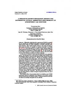
4. Analysis of the Rolling-Bearing on an Experimental Bench 4. Analysis of the Rolling-Bearing on an Experimental Bench Generally, the rolling-bearing is an important part of machinery. In the actual operation, the inner rolling-bearing an important partrelated of machinery. the actual operation, inner ring,Generally, the outerthe ring and rolling is element parts are to eachInother. Hence, there isthe a strong ring, the outer ring and rolling element parts are related to each other. Hence, there is a strong correlation between the different vibration sources. Limited by the testing experiment, one channel correlation between different in vibration Limited by the testing oneproposed channel observation signal isthe monitored normal sources. conditions. In order to verify theexperiment, validity of the observation signal is monitored normal In order to verify the validity the proposed method in the experiment, this in signal wasconditions. used to detect the coupling faults of theofinner and outer method experiment, this was used apparatus to detect the coupling faults theexperimental inner and outer ringsof rings ofinathe rolling-bearing. Thesignal experimental was provided byofthe center ofinstitute a rolling-bearing. The experimental providedof byScience the experimental center of institute of mechanical automation apparatus in Wuhanwas University and Technology, which is ofcustomized mechanicalby automation in Wuhan University of Science andwas Technology, which is customized by the the American SQi company. This apparatus composed of a motor drive, encoder, American SQi company. This apparatus was composed of a motor drive, encoder, and fault simulation and fault simulation of the two-level reduction gear box and load device. The specific device is ofshown the two-level reduction gear box and load device. The specific device is shown in Figure 10. in Figure 10.
(a)
1
2
3 4
5
(b) Figure 10. Fault simulation experimental table for the rolling-bearing of a gear box. (a) The physical Figure 10. Fault simulation experimental table for the rolling-bearing of a gear box. (a) The physical map of the test rig; (b) The structure diagram of the test rig: 1-motor, 2-encoder, 3-gearbox, 4-measured map of the test rig; (b) The structure diagram of the test rig: 1-motor, 2-encoder, 3-gearbox, 4-measured pointand and5-load 5-loaddevice. device. point
In this paper, the deep-groove ball bearing ER-16k (FAFNIR, Springfield, MA, USA) with faults In this paper, the deep-groove ball bearing ER-16k (FAFNIR, Springfield, MA,and USA) faults on the outer and inner rings was simulated. According to the bearing parameters thewith coefficient on the outer and inner rings was simulated. According to the bearing parameters and the coefficient of of the gear transmission ratio, the frequency of the inner ring and the outer ring of the bearing fault the gear transmission ratio, frequency were calculated, which arethe listed in Tableof3.the inner ring and the outer ring of the bearing fault were calculated, which are listed in Table 3. Table 3. Main characteristic frequencies of the SQi simulation test table. Table 3. Main characteristic frequencies of the SQi simulation test table.
Rotating Rotating Frequency Frequency f f
Transmission
Output
Inner Ring
Outer Ring
Transmission RingFrequency Fault Outer Ring Fault Frequency Output Frequency Frequency Inner Fault Fault Frequency Frequency Frequency Frequency
0.29f
0.29f
0.11f
0.11f
5.43f
5.43f
3.572f
3.572f
It is noted that f is the actual motor rotational frequency, which corresponds to the input shaft frequency. Motor rotating frequency was set to be 30 Hz. As the speed of the three-phase
Appl. Sci. 2017, 7, 414 Appl. Sci. 2017, 7, 414
13 of 18 13 of 18
It is noted that f iswill the actual motor frequency, corresponds to the shaft asynchronous motor fluctuate, therotational measured rotating which frequency is f 29 Hzinput in reality. frequency. Motor rotating frequency was set to be 30 Hz. As the speed of the three-phase asynchronous Hence, the characteristic frequencies of the inner and outer rings of the bearing can be calculated as motor will fluctuate, the measured rotating frequency is f = 29 Hz in reality. Hence, the characteristic fi 157.47 Hz and fo 103.59 Hz, which are shown in Table 4. The original time-domain frequencies of the inner and outer rings of the bearing can be calculated as f i = 157.47 Hz and and the measured single-channel are shown in Figure fwaveform = 103.59 Hz,frequency which arespectrum shown inofTable 4. The original time-domain waveform and11. frequency o spectrum of the measured single-channel are shown in Figure 11. Table 4. Characteristic frequencies of FAFNIR deep groove ball bearing.
Table 4. Characteristic FAFNIR deep groove bearing. Innerfrequencies Ring FaultofFrequency Outerball Ring Fault Frequency
Rotating Frequency f /Hz
Rotating Frequency f /Hz 29
29
f /Hz
Inner Ring Faulti Frequency f i /Hz
157.47
157.47
f /Hz
o Outer Ring Fault Frequency f o /Hz
130.59 130.59
(a)
(b) Figure 11. Time domain and frequency spectrum of a single channel composite signal. (a) The time Figure 11. Time domain and frequency spectrum of a single channel composite signal. (a) The time response of a measured single channel vibration signal; (b) The frequency domain of measured response of a measured single channel vibration signal; (b) The frequency domain of measured single single channel vibration signal. channel vibration signal.
In order to perform the blind source separation of a single-channel composite signal in the In orderstation, to perform the blindwas source of decompose a single-channel composite signalwith in the experiment the RPSEMD first separation employed to the composite signal, the experiment station, the RPSEMD was first employed to decompose the composite signal, with the mode components then being obtained. Subsequently, the original signal and the decomposed mode mode components being obtained. the original signalbefore and the mode components were then decomposed by SVDSubsequently, to obtain characteristic values, thedecomposed number of source components decomposed SVD to of obtain values, beforeobservation the numbersignal of source signals was were determined by thebymethod BIC.characteristic Following this, the new was processed by the proposed blind source separation and the analyzed result is drawn in Figure 12.
Appl. Sci. 2017, 7, 414
14 of 18
signals was determined by the method of BIC. Following this, the new observation signal was processed by theSci. proposed Appl. 2017, 7, 414blind source separation and the analyzed result is drawn in Figure 12. 14 of 18
(a)
(b) Figure 12. Result of blind source separation in the frequency domain provided by the proposed Figure 12. Result of blind source separation in the frequency domain provided by the proposed method. method. (a) The first component obtained by the proposed method. (b) The second component (a) The first component obtained by the proposed method. (b) The second component obtained by the obtained by the proposed method. proposed method.
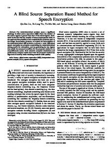
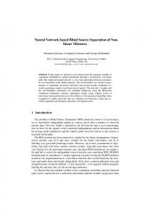
Figure 12a,b present the frequency spectrum of the estimated signal by the proposed method. Figure 12a,b present the frequency spectrum of the estimated signal by the proposed method. From Figure 12a, the rotating frequency f r and its double frequency 2 f r can be inspected. In From Figure 12a, the rotating frequency f r and its double frequency 2 f r can be inspected. In addition, f i , its double fi and its addition, the fault innerfrequency ring faultf i ,frequency frequency third harmonic the inner ring its double frequency 2 f i and its third 2 harmonic frequency 3 f i can also be identified. Moreover, the modulation phenomenon is rather obvious, which can further frequency 3 f i can also be identified. Moreover, the modulation phenomenon is rather obvious, prove fault of roll-bearing. Analogously, the outer ring faultthe frequency f o , fault its double and whichthe caninner further prove the inner fault of roll-bearing. Analogously, outer ring frequency triple frequencies can also be found in Figure 12b. Therefore, the method proposed in this paper can f o , its double and triple frequencies can also be found in Figure 12b. Therefore, the method accurately identify the fault frequency of the inner ring and the outer ring, which achieves the blind proposed in this of paper can accurately identify theinfault frequency oftable. the inner ring and the outer source separation a multi-fault composite signal the experimental ring,Inwhich achieves the blind source separation of a multi-fault signal in the the a similar way, the above-mentioned EEMD method for BSS [31] composite was compared with experimental table.with the result being plotted in Figure 13. Nevertheless, it has little difference proposed method, In a similar way, theand above-mentioned method for BSS [31] be was comparedBased with on the in the frequency domain only the inner EEMD ring fault frequency f i can identified. proposed method, with the result being plotted in Figure 13. Nevertheless, it has little difference in Figures 12 and 13, we can make the judgment that the proposed method performs better in actual, the frequency domain andseparation. only the inner ring fault frequency f i can be identified. Based on measured multi-fault signal Figures 12 and 13, we can make the judgment that the proposed method performs better in actual, measured multi-fault signal separation.
Appl. Sci. 2017, 7, 414 Appl. Sci. 2017, 7, 414
15 of 18 15 of 18
(a)
(b) Figure 13. Result of blind source separation provided by EEMD. (a) The first component obtained by Figure 13. Result of blind source separation provided by EEMD. (a) The first component obtained by EEMD; (b) The second component obtained by EEMD. EEMD; (b) The second component obtained by EEMD.
5. Conclusions 5. Conclusions Single-channel blind source separation algorithm (SCBSS) has important theoretical and Single-channel blind source separation algorithm (SCBSS) has important theoretical and practical practical values in the multi-fault feature extraction for mechanical equipment. The main work in values in theismulti-fault feature extraction equipment. The main work in this paper this paper summarized as follows: (1)forAmechanical novel regenerated phase-shifted sinusoid-assisted is summarized follows: (1) A(RPSEMD) novel regenerated sinusoid-assisted empirical mode empirical modeasdecomposition method phase-shifted was introduced for signal decomposition. It not decomposition (RPSEMD) method was introduced for signal decomposition. It not only inhibited only inhibited the mode mixing problem during the whole decomposition process, but also had the mode mixing problem during the whole process, also had superiority without superiority without parameter selection. Asdecomposition it produces the better but performance of adaptive signal parameter selection. As it produces the better performance of adaptive signal decomposition, it was decomposition, it was first applied to the blind source separation of a single-channel composite first applied to the blind source of a single-channel composite in health information monitoring signal in health monitoring of separation key mechanical equipment. (2) Based onsignal the Bayesian of key mechanical equipment; (2) Based on the Bayesian information criterion and singular value criterion and singular value characteristics generated by SVD model, the number of source signals characteristics generated by SVD model, the number of source signals was accurately estimated; was accurately estimated. (3) Through theoretical analysis and experimental tests, it was shown that (3) theoreticalinanalysis and experimental it was shown that the method proposed in theThrough method proposed this paper could effectivelytests, extract the fault features and solve the problems this paper could effectively extract the fault features and solve the problems of multi-fault separation. of multi-fault separation. Therefore, the proposed method could serve as a powerful tool in Therefore, proposed method could serve as a powerful tool in multi-fault identification. multi-faultthe identification.
Appl. Sci. 2017, 7, 414
16 of 18
Acknowledgments: This work was supported by the National Natural Science Foundation of China under Grants Nos. 51475339, 51405353 and 51105284; the Natural Science Foundation of Hubei province under Grant No. 2016CFA042 and the State Key Laboratory of Refractories and Metallurgy, Wuhan University of Science and Technology under Grant No. ZR201603. Author Contributions: Cancan Yi and Yong Lv conceived and designed the experiments; Cancan Yi and Han Xiao performed the experiments; Cancan Yi and Han Xiao analyzed the data; Cancan Yi and Guanghui You contributed reagents/materials/analysis tools; Cancan Yi and Zhang Dang wrote the paper. Conflicts of Interest: The authors declare no conflict of interest.
References 1. 2. 3. 4. 5.
6. 7. 8. 9. 10. 11.
12. 13. 14. 15. 16. 17.
18. 19.
Li, Y.; Xu, M.; Wang, R.; Huang, W. A fault diagnosis scheme for rolling bearing based on local mean decomposition and improved multiscale fuzzy entropy. J. Sound Vib. 2016, 360, 277–299. [CrossRef] Yi, C.; Lv, Y.; Dang, Z.; Xiao, H. A Novel Mechanical Fault Diagnosis Scheme Based on the Convex 1-D Second-Order Total Variation Denoising Algorithm. Appl. Sci. 2016, 6, 403. [CrossRef] Yi, C.; Lv, Y.; Dang, Z. A Fault Diagnosis Scheme for Rolling Bearing Based on Particle Swarm Optimization in Variational Mode Decomposition. Shock Vib. 2016, 2016, 9372691. [CrossRef] Xu, B.; Song, G.; Masri, S.F. Damage detection for a frame structure model using vibration displacement measurement. Struct. Health Monit. 2012, 11, 281–292. [CrossRef] Yao, P.; Kong, Q.; Xu, K.; Jiang, T.; Hou, L.; Song, G. Structural health monitoring of multi-spot welded joints using a lead zirconate titanate based active sensing approach. Smart Mater. Struct. 2016, 25, 015031. [CrossRef] Zhang, L.; Wang, C.; Song, G. Health Status Monitoring of Cuplock Scaffold Joint Connection Based on Wavelet Packet Analysis. Shock Vib. 2015, 2015, 695845. [CrossRef] Feng, Q.; Kong, Q.; Huo, L.; Song, G. Crack detection and leakage monitoring on reinforced concrete pipe. Smart Mater. Struct. 2015, 24, 115020. [CrossRef] Li, D.; Ho, S.C.M.; Song, G.; Ren, L.; Li, H. A review of damage detection methods for wind turbine blades. Smart Mater. Struct. 2015, 24, 033001. [CrossRef] Yi, C.; Lv, Y.; Dang, Z.; Xiao, H.; Yu, X. Quaternion singular spectrum analysis using convex optimization and its application to fault diagnosis of rolling bearing. Measurement 2017, 103, 321–332. [CrossRef] Belouchrani, A.; Abed-Meraim, K.; Cardoso, J.F.; Moulines, E. A blind source separation technique using second-order statistics. IEEE Trans. Signal Process. 1997, 45, 434–444. [CrossRef] Zhao, M.; Lin, J.; Xu, X.Q.; Li, X.J. Multi-fault detection of rolling element bearings under harsh working condition using IMF-based adaptive envelope order analysis. Sensors 2014, 14, 20320–20345. [CrossRef] [PubMed] Kouadri, A.; Baiche, K.; Zelmat, M. Blind source separation filters-based-fault detection and isolation in a three tank system. J. Appl. Stat. 2014, 41, 1799–1813. [CrossRef] Antoni, J. Blind separation of vibration components: Principles and demonstrations. Mech. Syst. Signal Process. 2005, 19, 1166–1180. [CrossRef] Gelle, G.; Colas, M.; Serviere, C. Blind source separation: A tool for rotating machine monitoring by vibrations analysis? J. Sound Vib. 2001, 248, 865–885. [CrossRef] Mowlaee, P.; Christensen, M.G.; Jensen, S.H. New results on single-channel speech separation using sinusoidal modeling. IEEE Trans. Audio Speech Lang. Process. 2011, 19, 1265–1277. [CrossRef] Gao, B.; Woo, W.L.; Dlay, S.S. Single channel source separation using EMD-subband variable regularized sparse features. IEEE Trans. Audio Speech Lang. Process. 2011, 19, 961–976. [CrossRef] Guo, Y.; Naik, G.R.; Nguyen, H. Single channel blind source separation based local mean decomposition for Biomedical applications. In Proceedings of the 2013 35th Annual International Conference of the IEEE, Osaka, Japan, 3–7 July 2013; pp. 6812–6815. Guo, Y.; Huang, S.; Li, Y.; Naik, G.R. Edge effect elimination in single-mixture blind source separation. Circuits Syst. Signal Process. 2013, 32, 2317–2334. [CrossRef] Pendharkar, G.; Naik, G.R.; Nguyen, H.T. Using blind source separation on accelerometry data to analyze and distinguish the toe walking gait from normal gait in ITW children. Biomed. Signal Process. Control 2014, 13, 41–49. [CrossRef]
Appl. Sci. 2017, 7, 414
20. 21.
22.
23.
24. 25. 26. 27.
28. 29. 30.
31.
32. 33. 34.
35. 36.
37.
38. 39. 40.
17 of 18
Davies, M.E.; James, C.J. Source separation using single channel ICA. Signal Process. 2007, 87, 1819–1832. [CrossRef] Chai, R.; Naik, G.; Nguyen, T.N.; Ling, S.; Tran, Y.; Craig, A.; Nguyen, H. Driver Fatigue Classification with Independent Component by Entropy Rate Bound Minimization Analysis in an EEG-based System. IEEE J. Biomed. Health Inform. 2016. [CrossRef] [PubMed] Wang, C.; Chen, J.; Xiao, F. Application of Empirical Model Decomposition and Independent Component Analysis to Magnetic Anomalies Separation: A Case Study for Gobi Desert Coverage in Eastern Tianshan, China. In Geostatistical and Geospatial Approaches for the Characterization of Natural Resources in the Environment; Springer International Publishing: Berlin, Germany, 2016. Naik, G.; Altimemy, A.; Nguyen, H. Transradial Amputee Gesture Classification Using an Optimal Number of sEMG Sensors: An Approach Using ICA Clustering. IEEE Trans. Neural Syst. Rehabil. Eng. 2015, 24, 1–10. [CrossRef] [PubMed] Maneshi, M.; Vahdat, S.; Gotman, J.; Grova, C. Validation of Shared and Specific Independent Component Analysis (SSICA) for Between-Group Comparisons in fMRI. Front. Neurosci. 2016, 10. [CrossRef] [PubMed] Di Persia, L.E.; Milone, D.H. Using multiple frequency bins for stabilization of FD-ICA algorithms. Signal Process. 2016, 119, 162–168. [CrossRef] Adali, T.; Calhoun, V.D. Complex ICA of brain imaging data. IEEE Signal Process. Mag. 2007, 24, 136. [CrossRef] Naik, G.R.; Kumar, D.K. Estimation of independent and dependent components of non-invasive EMG using fast ICA: Validation in recognising complex gestures. Comput. Methods Biomech. Biomed. Eng. 2011, 14, 1105–1111. [CrossRef] [PubMed] Guo, J.; Deng, Y. A Time-Frequency Algorithm for Noisy ICA. In Geo-Informatics in Resource Management and Sustainable Ecosystem; Springer: Berlin/Heidelberg, Germany, 2015; pp. 357–365. Hong, H.; Liang, M. Separation of fault features from a single-channel mechanical signal mixture using wavelet decomposition. Mech. Syst. Signal Process. 2007, 21, 2025–2040. [CrossRef] Mijovi´c, B.; de Vos, M.; Gligorijevic, I.; Taelman, J.; Van Huffel, S. Source separation from single-channel recordings by combining empirical-mode decomposition and independent component analysis. IEEE Trans. Biomed. Eng. 2010, 57, 2188–2196. [CrossRef] [PubMed] Naik, G.R.; Selvan, S.E.; Nguyen, H.T. Single-Channel EMG Classification with Ensemble-EmpiricalMode-Decomposition-Based ICA for Diagnosing Neuromuscular Disorders. IEEE Trans. Neural Syst. Rehabil. Eng. A Publ. IEEE Eng. Med. Biol. Soc. 2016, 24, 734–743. [CrossRef] [PubMed] Zhao, X.; Li, M.; Song, G.; Xu, J. Hierarchical ensemble-based data fusion for structural health monitoring. Smart Mater. Struct. 2010, 19, 126–134. [CrossRef] Lv, Y.; Yuan, R.; Song, G. Multivariate empirical mode decomposition and its application to fault diagnosis of rolling bearing. Mech. Syst. Signal Process. 2016, 81, 219–234. [CrossRef] Sadhu, A. An Integrated Multivariate Empirical Mode Decomposition Method towards Modal Identification of Structures. Available online: http://journals.sagepub.com/doi/abs/10.1177/1077546315621207 (accessed on 7 January 2017). Wu, Z.; Huang, N.E. Ensemble empirical mode decomposition: A noise-assisted data analysis method. Adv. Adapt. Data Anal. 2009, 1, 1–41. [CrossRef] Wang, H.; Li, R.; Tang, G.; Yuan, H.F.; Zhao, Q.L.; Cao, X. A compound fault diagnosis for rolling bearings method based on blind source separation and ensemble empirical mode decomposition. PLoS ONE 2014, 9, e109166. [CrossRef] [PubMed] Guo, Y.; Huang, S.; Li, Y. Single-mixture source separation using dimensionality reduction of ensemble empirical mode decomposition and independent component analysis. Circuits Syst. Signal Process. 2012, 31, 2047–2060. [CrossRef] Yeh, J.R.; Shieh, J.S.; Huang, N.E. Complementary Ensemble Empirical Mode Decomposition: A Novel Noise Enhanced Data Analysis Method. Adv. Adapt. Data Anal. 2011, 2, 135–156. [CrossRef] Kouchaki, S.; Sanei, S.; Arbon, E.L.; Dijk, D.J. Tensor based singular spectrum analysis for automatic scoring of sleep EEG. IEEE Trans. Neural Syst. Rehabil. Eng. 2015, 23, 1–9. [CrossRef] [PubMed] Wang, C.; Kemao, Q.; Da, F. Regenerated Phase-Shifted Sinusoid-Assisted Empirical Mode Decomposition. IEEE Signal Process. Lett. 2016, 23, 556–560. [CrossRef]
Appl. Sci. 2017, 7, 414
41. 42. 43. 44.
18 of 18
Huang, L.; Xiao, Y.; Liu, K.; So, H.C. Bayesian information criterion for source enumeration in large-scale adaptive antenna array. IEEE Trans. Veh. Technol. 2016, 65, 3018–3032. [CrossRef] Cardoso, J.F.; Souloumiac, A. Blind Beamforming for non-Gaussian Signals. IEE Proc. F Radar Signal Process. 1994, 140, 362–370. [CrossRef] Ypma, A. Learning Methods for Machine Vibration Analysis and Health Monitoring; TU Delft: Delft, The Netherlands, 2001. Randall, R.B.; Antoni, J.; Chobsaard, S. The relationship between spectral correlation and envelope analysis in the diagnostics of bearing faults and other cyclostationary machine signals. Mech. Syst. Signal Process. 2001, 15, 945–962. [CrossRef] © 2017 by the authors. Licensee MDPI, Basel, Switzerland. This article is an open access article distributed under the terms and conditions of the Creative Commons Attribution (CC BY) license (http://creativecommons.org/licenses/by/4.0/).