In this chapter we consider the negotiation over the contents of a bundle of items (thus we use the term âmulti-itemâ negotiation), though, at a conceptual level, ...
Retrieving the Structure of Utility Graphs Used in Multi-Item Negotiation through Collaborative Filtering of Aggregate Buyer Preferences Valentin Robu, Han La Poutr´e CWI, Dutch National Research Center for Mathematics and Computer Science Kruislaan 413, NL-1098 SJ Amsterdam, The Netherlands {robu, hlp}@cwi.nl Summary. Graphical utility models represent powerful formalisms for modeling complex agent decisions involving multiple issues [3]. In the context of negotiation, it has been shown [14] that using utility graphs enables agents to reach Pareto-efficient agreements with a limited number of negotiation steps, even for high-dimensional negotiations over bundles of items involving non-linear complementarity/ substitutability dependencies. This chapter considerably extends the results of our previous work [14], by proposing a method for constructing the utility graphs of buyers automatically, based on previous negotiation data. Our method is based on techniques inspired from item-based collaborative filtering, widely used in online recommendation algorithms. Experimental results show that our approach is able to retrieve the structure of utility graphs online, with a relatively high degree of accuracy, even for complex non-linear settings and even if a relatively small amount of data about concluded negotiations is available. Therefore, this chapter establishes a formal link between preference modeling techniques used in automated negotiation and preference modeling techniques used in social filtering.
1 Introduction Negotiation represents a key form of interaction between providers and consumers in electronic markets. One of the main benefits of negotiation in e-commerce is that it enables greater customization to individual customer preferences, and it supports buyer decisions in settings which require agreements over complex contracts. Automating the negotiation process, through the use of intelligent agents which negotiate on behalf of their owners, enables electronic merchants to go beyond price competition by providing flexible contracts, tailored to the needs of individual buyers. Multi-issue (or multi-item) negotiation models are particularly useful for this task, since with multi-issue negotiations mutually beneficial (”win-win”) contracts can be found [7, 18, 8, 11, 10]. In this chapter we consider the negotiation over the contents of a bundle of items (thus we use the term “multi-item” negotiation), though, at a conceptual level, the setting is virtually identical to previous work on
2
V. Robu, J.A. La Poutr´e
multi-issue negotiation involving only binary-valued issues (e.g. [8]). A bottleneck in most existing approaches to automated negotiation is that they only deal with linearly additive utility functions, and do not consider high-dimensional negotiations and in particular, the problem of interdependencies between evaluations for different items. This is a significant problem, since identifying and exploiting substitutability/complementarity effects between different items can be crucial in reaching mutually profitable deals. 1.1 Automated multi-item negotiation vs. combinatorial auctions and preference elicitation The problems addressed through multi-item negotiation have also been approached, in the multi-agent research community, through a variety of other methods. Auctions are a method of choice, in particular when (a set of) scarce items or resources needs to be allocated among a group of self-interested agents. However, as shown in [12], when applied to many e-commerce settings, auctions often suffer from problems such as as “winner’s curse” or delays in the buyer acquiring the goods. In an auction, a set of buyers compete for buying a scarce good (or sets of goods), while the business model of most e-commerce merchants involves increasing the sale volumes by encouraging customers not to compete against each other, but to explore the ”long tail” of their product range (often done by offering customized discounts). Combinatorial auctions are a special category of auctions that have been successfully applied to a wide variety of problems. For example, for the particular preference language we consider (i.e. k-wise additive preferences), an algorithm for winner determination has recently been proposed in [4]. However, in many practical applications, a bottleneck of combinatorial auctions is that parties must reveal their full preferences over all possible bundles before the auction begins. By contrast, in automated negotiation, the preferences of the parties are not revealed in advance: usually a model of the opponent’s (i.e. negotiation partner) preferences has to be learned from his/her past bids. Thus we can say that auctions are direct revelation mechanisms, while automated negotiations are indirect revelation ones. Another line of work, directly related to ours, is preference elicitation. There is, indeed, a strong link between models used in preference elicitation and multi-item negotiation. For example, Brazunias and Boutilier [1] propose a model (developed independently and concurrently with our work), for utility elicitation in generalized additive independence (GAI) models. There are, however, also important differences. First, the model proposed in [1] uses a different graphical formalism to encode preferences, while their optimization criteria is the error in reached in the utility of the buyer, not Pareto efficiency. In preference elicitation settings, the prices asked by the seller are fixed throughout the process and are known to the oracle (for our setting, the oracle roughly corresponds to the buyer agent, i.e. the party whose preferences need to be modelled or learned). By contrast, negotiation is usually a game with double-sided incomplete information. Although the parties start from an initial vector of asking prices, the buyer has an incentive not only to explore the bundle contents, but also to bargain about the price of the bundle being offered (according
Retrieving the Structure of Utility Graphs Used in Multi-Item Negotiation
3
to his/her negotiation strategy). Finally, in [1] (just as in our previous work [14]), the problem of acquiring the initial graphical model structure is left for future research. It is exactly this problem that is covered in this book chapter, as an extension of our negotiation model presented in [14]. It could be argued there is also a relation between multi-item negotiation as discussed in this chapter and computational approaches to argumentation-based negotiation. We leave the study of this issue to further work. 1.2 Using utility graphs to model negotiations over bundles of items In our previous work [14], in order to to model buyer preferences in high-dimensional negotiations, we have introduced the concept of utility graphs. Intuitively defined, a utility graph (UG) is a structural model of a buyer, representing a buyer’s perception of dependencies between two items (i.e. whether the buyer perceives two items to be as complementary or substitutable). An estimation of the buyer’s utility graph can be used by the seller to efficiently compute the buyer’s utility for a “bundle” of items, and propose a bundle and price based on this utility. The main result presented in [14] is that Pareto-efficient agreements can be reached, even for high dimensional negotiations with a limited number of negotiation steps, but provided that the seller starts the negotiation with a reasonable approximation of the structure of the true utility graph of the type of buyer he is negotiating with (i.e. he has a reasonable idea which issues or items may be complimentary or substitutable in the evaluation of buyers in his domain). The seller agent can then use this graph to negotiate with a specific buyer. During this negotiation, the seller will adapt the weights and potentials in the graph, based on the buyer’s past bids. However, this assumes the seller knows a super-graph of the utility graphs of the class of buyers he is negotiating with (i.e. a graph which subsumes the types of dependencies likely to be encountered in a given domain - c.f. Sec. 2.2). Due to space limitations, and to avoid too much overlap in content with our previous AAMAS paper [14], in this chapter we do not describe the full negotiation model, the way seller weights are updated throughout the process, the initialisation settings etc. These results have been described in [14], and we ask the intrested reader to consult this work. An important issue left open in [14] is how does the seller acquire this initial graph information. One method would be to elicit it from human experts (i.e. an e-commerce merchant is likely to know which items are usually sold together or complimentary in value for the average buyer and which items are not). For example, if the electronic merchant is selling pay-per-item music tunes, the tunes from the same composer or performer can be potentially related. In this chapter, we show this can also be retrieved automatically, by using information from completed negotiation data. The implicit assumption we use here is that buyer preferences are in some way clustered, i.e. by looking at buyers that have shown interest for the same combinations of items in the past, we can make a prediction about future buying patterns of the current customer. Note that this assumption
4
V. Robu, J.A. La Poutr´e
is not uncommon: it is a building block of most recommendation mechanisms deployed in Internet today [17]. In order to generate this initial structure of our utility graph, in this chapter we propose a technique inspired by collaborative filtering. Furthermore, compared to an initial version of this work, presented in [19], we are now able to more rigorously define and test a cut-off criterion for selecting graph edges for a wide category of graphs. 1.3 Collaborative filtering Collaborative filtering [17] is the main underlying technique used to enable personalization and buyer decision aid in today’s e-commerce, and has proven very successful both in research and practice. The main idea of collaborative filtering is to output recommendations to buyers, based on the buying patterns detected from buyers in previous buy instances. There are two approaches to this problem. The first of these is use of the preference database to discover, for each buyer, a neighborhood of other buyers who, historically, had similar preferences to the current one. This method has the disadvantage that it requires storing a lot of personalized information and is not scalable (see [17]). The second method, of more relevant to our approach, is item-based collaborative filtering. Item based techniques first analyze the user-item matrix (i.e. a matrix which relates the users to the items they have expressed interest in buying), in order to identify relationships between different items, and then use these to compute recommendations to the users [17]. In our case, of course, the recommendation step is completely replaced by negotiation. What negotiation can add to such techniques is that enables a much higher degree of customization, also taking into account the preferences of a specific customer. For example, a customer expressing an interest to buy a book on Amazon is sometimes offered a ”special deal” discount on a set (bundle) of books, including the one he initially asked for. The potential problem with such a recommendation mechanism is that it’s static: the customer can only take it, leave it or stick to his initial buy, it cannot change slightly the content of the suggested bundle or try to negotiate a better discount. By using negotiation a greater degree of flexibility is possible, because the customer can critique the merchant’s sub-optimal offers through her own counter-offers, so the space of mutually profitable deals can be better explored. 1.4 Paper structure and relationship to previous work The paper is organized as follows. In Section 2 we briefly present the general setting of our negotiation problem, define the utility graph formalism and the way it can be used in negotiations. Section 3 describes the main result of the chapter, namely how the structure of utility graphs can be elicited from existing negotiation data. Section 4 presents the experimental results from our model, while Section 5 concludes with a discussion. An important issue to discuss is the relationship of this book chapter with our previous work. In our paper at the AAMAS’05 conference [14], we first introduced
Retrieving the Structure of Utility Graphs Used in Multi-Item Negotiation
5
the utility graph formalism and present an algorithm that exploits the decomposable structure of such graphs in order to reach faster agreements during negotiation. That paper, however, uses the assumption that a minimal super-graph of individual buyer graphs is already available to the seller at the start of the negotiation. In a paper at the PRIMA’05 conference [19] we provide the first discussion of how different collaborative filtering criteria could be used to build the structure of this super-graph. This book chapter builds on and considerably extends these results, by proposing and testing a rigorous criteria for selecting a number of edges returned by the collaborative filtering process. This enables us to extend our approach to a much wider category of graphs. We admit that there is some overlap in content, especially with [19], but we feel this cannot be avoided in order for the reader to understand the context and functionality of our model. We stress, however, that around 50% of the material and the experimental results presented are completely new to this book chapter. For lack of space, we cannot present the full negotiation model from [14] in this chapter, except at a very general level, since we prefer to concentrate on describing the new results. The interested reader is therefore asked to consult [14] for further details.
2 The multi-issue negotiation setting In this section we give some background information of the set-up of our model. First we give a formal definition of the concept of utility graphs. Next we describe (very briefly) how this formalism can be used in negotiation (a issue fully discussed in [14]). Finally we discuss how the learning of the structure from past data is integrated with the negotiation part. 2.1 Utility Graphs: Definition and Example We consider the problem of a buyer who negotiates with a seller over a bundle of n items, denoted by B = {I1 , . . . , In }. Each item Ii takes on either the value 0 or 1: 1 (0) means that the item is (not) purchased. The utility function u : Dom(B) 7→ R specifies the monetary value a buyer assigns to the 2n possible bundles (Dom(B) = {0, 1}n). In traditional multi-attribute utility theory, u would be decomposable as the sum of utilities over the individual issues (items) [13]. However, in this chapter we follow the previous work of [3] by relaxing this assumption; they consider the case where u is decomposable in sub-clusters of individual items such that u is equal to the sum of the sub-utilities of different clusters. Definition 1. Let C be a set of (not necessarily disjoint) clusters of items C1 , . . . , Cr (with Ci ⊆ B). We say that a utility function is factored according to C if there |Ci| exists functions Pui : Dom(Ci ) 7→ R (i = 1, . . . , r and Dom(Ci ) = {0, 1} ) such that u(b) = i ui (ci ) where b is the assignment to the variables in B and ci is the corresponding assignment to variables in Ci .We call the functions ui sub-utility functions.
6
V. Robu, J.A. La Poutr´e
We use the following factorization, which is a relatively natural choice within the context of negotiation. Single-item clusters (|Ci | = 1) represent the individual value of purchasing an item, regardless of whether other items are present in the same bundle. Clusters with more than one element (|Ci | > 1) represent the synergy effect of buying two or more items; these synergy effects are positive for complementary items and negative for substitutable ones. In this chapter, we restrict our attention to clusters of size 1 and 2 (|Ci | ∈ {1, 2}, ∀i). This means we only consider binary item-item complementarity/substitutability relationships, though the case of retrieving larger clusters could form the object of future research. The factorization defined above can be represented as an undirected graph G = (V, E), where the vertexes V represent the set of items I under negotiation. An arc between two vertexes (items) i, j ∈ V is present in this graph if and only if there is some cluster Ck that contains both Ii and Ij . We will henceforth call such a graph G a utility graph. Example 1. Let B = {I1 , I2 , I3 , I4 } and C = {{I1 }, {I2 }, {I1 , I2 }, {I2 , I3 }, {I2 , I4 }} such that ui is the sub-utility function associated with cluster i (i = 1, . . . , 5). Then the utility of purchasing, for instance, items I1 , I2 , and I3 (i.e., b = (1, 1, 1, 0)) can be computed as follows: u((1, 1, 1, 0)) = u1 (1) + u2 (1) + u3 ((1, 1)) + u4 ((1, 1)), where we use the fact that u5 (1, 0) = u5 (0, 1) = 0 (synergy effect only occur when two or more items are purchased). The utility graph of this factorization is depicted in Fig. 1.
+
I3
I1
I2
+
I4
Fig. 1. The utility graph that corresponds to the factorization according to C in Example 1. The + and − signs on the edges indicate whether the synergy represents a complementarity, respectively substitutability effect.
Stated less formally, in our graphical model the dependency expressed by an arc (or hyper-arc) between 2 or more items encodes only an additional potential compared to all sub-combinations included in the sub-bundle. Thus, for the specific case of 2-additive dependencies (which can be expressed by two-ended, undirected arcs), we assign an individual utility to each item and, for each pair of items with a complementarity/substitutability dependency, we assign a value for the strength of the dependency (either positive or negative). The utility of any bundle combination will be the sum of utilities for all individual items present in the bundle, plus the value of all bilateral dependencies, for which both items are instantiated with “1” (present) in the given bundle. The advantage of this method (compared to other graphical
Retrieving the Structure of Utility Graphs Used in Multi-Item Negotiation
7
formalisms, e.g. [1]) is that we only need to use addition over the values of individual items and non-linearity effects in order to compute the utility of a bundle, while they alternate the + and - signs in the summation. 2.2 Minimal super-graph for a class of buyers The definition of utility graphs given in Section 2.1 corresponds to the modeling the utility function of an individual buyer. In this chapter, we call the utility graph of an individual buyer the underlying or true graph (to distinguish it from the retrieved or learned graph, reconstructed through our method). The underlying graph of any buyer remains hidden from the seller throughout the negotiation. We do assume, however, that the buyers which negotiate with a given electronic merchant belong to a certain class or population of buyers. This means the utility buyers assign to different bundles of items follow a certain structure, specific to a buying domain (an assumption also used indirectly in [18, 7, 17]). Buyers from the same population are expected to have largely overlapping graphs, though not all buyers will have all interdependencies specific to the class. Definition 2. Let A = {A1 , ..An } be a set (class, population) of n buyers. Each buyer i = 1..n has a utility function ui , which can be factored according to a set of clusters Ci = {Ci,1 , Ci,2 ..CI,r(i) }. We define the super-set of clusters for the class of buyers A = {A1 , ..An } as: CA = C1 ∪ C2 ∪ .. ∪ Cn . In graph-theoretic terms (as shown in Section 2.1), the set of clusters Ci according to which the utility a buyer Ai is structured is represented by a utility graph Gi , where each binary cluster from {Ci,1 , ..CI,r(i) } represents a dependency or an edge in the graph. The super-set of buyer clusters CA can also be represented by a graph GA , which is the minimal super-graph of graphs Gi , i = 1..n. This graph is called minimal because it contains no other edges than those corresponding to a dependency in the graph of at least one buyer agent from this class. We illustrate this concept by a very simple example, which also relies on Fig. 1. Example 2. Suppose we have 2 buyer agents A1 and A2 (obviously, this is a simplification, since a class would normally contain many more buyer graphs). Suppose the utility function of buyer A1 can be factored according to the clusters C1 = {{I1 }, {I2 }, {I2 , I3 }, {I2 , I4 }}, while the utility of A2 is factored according to C2 = {{I1 , I2 }, {I2 , I3 }, {I3 }}. Then the minimal utility super-graph for class A is given by: C1 = {{I1 }, {I2 }, {I3 }, {I1 , I2 }, {I2 , I3 }, {I2 , I4 }}. This super-graph is minimal, because is we were to add the dependency {I1 , I3 } to CA we would also obtain a super-graph, though not the minimal one. It is important to note that the above definition for the utility super-graph for a class of buyer refers only to the structure (i.e. clusters Ci ) and makes no assumption about the sub-utility values (i.e. functions ui ) in these clusters. To illustrate the difference, suppose that at a structural level, there is a complementarity effect between two items. However, for some buyers in the population, the utility value corresponding to this dependency may be very high (i.e. it is important for the agent to get both items), while for others it is much more moderate (or even close to zero).
8
V. Robu, J.A. La Poutr´e
2.3 Application to negotiation The negotiation, in our model, follows an alternating offers protocol. At each negotiation step each party (buyer/seller) makes an offer which contains an instantiation with 0/1 for all items in the negotiation set (denoting whether they are/are not included in the proposed bundle), as well as a price for that bundle. The decision process of the seller agent, at each negotiation step, is composed of 3 inter-related parts: (1) take into account the previous offer made by the other party, by updating his estimated utility graph of the preferences of the other party, (2) compute the contents (i.e. item configuration) of the next bundle to be proposed, and (3) compute the price to be proposed for this bundle. An important part of our model is that the burden of exploring the exponentially large bundle space and recommending profitable solutions is passed to the seller, who must solve it by modeling the preferences of his buyer (this is a reasonable model in e-commerce domains, where electronic merchants typically are more knowledgeable than individual buyers [7, 18]). The model the seller maintains of his buyer is represented by a utility graph, and tailors this graph towards the preferences of a given buyer, based on his/her previous offers. The seller does not know, at any stage, the values in the actual utility graph of the buyer, he only has an approximation learned after a number of negotiation steps. However, the seller does have some prior information to guide his opponent modeling. He starts the negotiation by knowing a super-graph of possible interdependencies between the issues (items) which can be present for the class of buyers he may encounter. The utility graphs of buyers form subgraphs of this graph. Note that this assumption says nothing about values of the sub-utility functions, so the negotiation is still with double-sided incomplete information (i.e. neither party has full information about the preferences of the other). In [14] we show how the presence of this graph helps to greatly reduce the complexity of the search space on the side of the seller. In [14] we argued that the structure of the minimal super-graph of the class of buyers likely to be encountered during negotiations can be obtained either from human experts or automatically, from a history of past negotiations, but in [14] we proposed no concrete mechanism how can this be achieved. It is this open problem that forms the subject of this chapter. 2.4 Overview of our approach There are two main stages of our approach(see also Figure 2): 1. Using information from previously concluded negotiations to construct the structure of the utility super-graph. In this phase the information used (past negotiation data) refers to a class of buyers and is not traceable to individuals. 2. The actual negotiation, in which the seller, starting from a super-graph for a class (population) of buyers, will negotiate with an individual buyer, drawn at random from the buyer population above. In this case, learning occurs based on the buyer’s previous bids during the negotiation, so information is buyer-specific.
Retrieving the Structure of Utility Graphs Used in Multi-Item Negotiation
9
However, this learning at this stage is guided by the structure of the super-graph extracted in the first phase.
Fig. 2. Top-level view of our agent architecture and simulation model
Phase 2 is described in our previous work [14]. The rest of this chapter will focus on describing the first phase of our model, namely retrieving the structure of the utility super-graph from previous data.
3 Constructing the Structure of Utility Graphs Using Concluded Negotiation Data Suppose the seller starts by having a dataset with information about previous concluded negotiations. This dataset may contain complete negotiation traces for different buyers, or we may choose, in order to minimize bias due to uneven-length negotiations, to consider only one record per negotiation. This can be either the first bid of the buyer or the bundle representing the outcome of the negotiation (for details
10
V. Robu, J.A. La Poutr´e
regarding how this negotiation data is generated and buyer profiles for the simulated negotiations are generated, please see the experimental set-up description in Section 4). The considered dataset is not personalized, i.e. the data which is collected online cannot be traced back to individual customers (this is a reasonable assumption in e-commerce, where storing a large amount of personalized information may harm customer privacy). However, in constructing of the minimal utility graph which the customers use, we implicitly assume that customers’ preference functions are related - i.e. their corresponding utility graphs, have a (partially) overlapping structure. Our goal is to retrieve the minimal super-graph of utility interdependencies which can be present for the class or population of buyers from which the negotiation data was generated. We assume that past data can be represented as a N ∗ n matrix, where N is the number of previous negotiation instances considered (e.g. up to 3000 in the tests reported in this chapter) and n is the number of issues (e.g. 50 for our tests). All the data is binary (i.e. with values of ”1” in the case the buyer asked for this item or ”0” if he does not). Item-based collaborative filtering [17] works by computing ”similarity measures” between all pairs of items in the negotiation set. The steps used are: 1. Compute raw item-item statistics (i.e. from existing negotiation data) 2. Compute item-item similarity matrices (from the raw statistics) 3. Compute qualitative utility graph, by selecting which dependencies to consider from the similarity matrices. In the following, we will examine each of these separately. 3.1 Computing the ”raw” statistic matrices Since what we need to compute is item-item similarity measures, we extract from this data some much smaller (n*n tables) which are sufficient to compute the required measures. We use the following notations throughout this chapter: • •
•
N for the total number of previous negotiation outcomes considered For each item i=1..n, Ni (1) and Ni (0) represent the number of times the item was (respectively was not) asked by the buyer, from the total of N previous negotiations For each pair of issues i, j = 1..n we denote by Ni,j (0, 0), Ni,j (0, 1), Ni,j (1, 0) and Ni,j (1, 1) all possibilities of joint acquisition (or non acquisition) of items i and j.
From the above definitions, the following property results immediately: Ni,j (0, 0)+ Ni,j (0, 1) + Ni,j (1, 0) + Ni,j (1, 1) = Ni (0) + Ni (1) = Nj (0) + Nj (1) = N , for all items i, j = 1..n. 3.2 Computing the similarity matrices The literature on item-based collaborative filtering defines two main criteria that could be used to compute the similarity between pairs of items: cosine-based and
Retrieving the Structure of Utility Graphs Used in Multi-Item Negotiation
11
correlation-based similarity. In our approach to the problem we have considered both of them and we report the detailed comparison results in [19]. However, from our experiments, only correlation-based similarity seems to perform well for this task, especially since we need to detect not only complementarity effects, but also substitutability ones. Cosine-based similarity is conceptually simpler, and, from our experience, works well in detecting complementarity dependencies and only in the case when the data is relatively sparse (each buyer expresses interest only in a few items). Correlation-based similarity, however, does not have these limitations. Therefore, in this chapter, we report the formulas and experimental results only for correlation-based similarity. Since the mathematical definitions (as presented in [17]) is given for real-valued preference ratings, we derive a more simplified form for the binary values case. Correlation-based similarity For correlation-based similarity, just one similarity matrix is computed containing both positive and negative values (to be more precise between -1 and 1). We first we define for each item i = 1..n, the average buy rate: Avi =
Ni (1) N
(1)
The following two terms are defined: ψ1 =
Ni,j (0, 0) ∗ Avi ∗ Avj − Ni,j (0, 1) ∗ Avi ∗ (1 − Avj ) −Ni,j (1, 0) ∗ (1 − Avi ) ∗ Avj + Ni,j (1, 1) ∗ (1 − Avi ) ∗ (1 − Avj )
and the normalization factor: r r Ni (0) ∗ Ni (1) Nj (0) ∗ Nj (1) ψ2 = ∗ N N The values in the correlation-based similarity matrix are then computed as: Sim(i, j) =
ψ1 ψ2
(2)
3.3 Building the super-graph of buyer utilities After constructing the similarity matrices, the next step is to use this information to build the utility super-graph for the class of buyers likely to be encountered in future negotiations. This amounts to deciding which of the item-item relationships from the similarity matrices should be included in this graph. For both similarity measures, higher values (i.e. closer to 1) represent stronger potential complementarity. For substitutability detection, the cosine similarity uses a different matrix, while the correlation-based it is enough to select values closer to -1.
12
V. Robu, J.A. La Poutr´e
Ideally, all the inter-dependencies corresponding to the arcs in the graph representing the true underlying preferences of the buyer should feature among the highest (respectively the lowest) values in the retrieved correlation tables. When an interdependency is returned that was not actually in the true graph, we call this is an excess (extra, erroneous) arc or interdependency. Due to noise in the data, it is unavoidable that a number of such excess arcs are returned. For example, if item I1 has a complimentary value with I2 and I2 is substitutable with I3 , it may be that items I1 and I3 often do not appear together, so the algorithm detects a substitutability relationship between them, which is in fact erroneous. The question on the part of the seller is: how many dependencies should be considered from the ones with highest correlation, as returned by the filtering algorithm? There are two aspects that affect this cut-off decision: •
•
If too few dependencies are considered, then it is very likely that some dependencies (edges) that are in the true underlying graph of the buyer will be missed. This means that the seller will ignore some interdependencies in the negotiation stage completely, which can adversely affect the Pareto-efficiency of the reached agreements. If too many dependencies are considered, then the initial starting super-graph of the seller will be considerably more dense than the “true” underlying graph of the buyer (i.e. it contains many excess or extra edges). Actually, this is always the case to some degree, and in [14] we claim that Pareto-efficient agreements can be reached starting from a super-graph of the buyer graphs. However, this supergraph cannot be of unlimited size. For example, starting from a graph close to full connectivity (i.e. with n2 edges for a graph with n issues or vertexes) would be equivalent to providing no prior information to guide the negotiation process.
In the general case, we consider graphs whose number of edges (or dependencies) is a linear in the number of items (issues) in the negotiation set. Otherwise stated, we restrict our attention to graphs in which the number of edges considered is some linear factor k times the number of items (vertexes) negotiated on. Framed in this way, the problem becomes of choosing the optimal value for parameter k (henceforth denoted by kopt ). In the previous version of this work [19] we “hard-coded” the choice of of kopt to a value of 2 and we provide results only for a category of graphs that have a maximum number of edges of 2 ∗ n (where n is the number of vertexes or items). In this chapter, however, we provide a method for choosing the value of kopt in the general case, which can be applied to a wider category of graphs. 3.4 Minimization of expected loss in Gains from Trade as cut-off criteria Denote by Nmissing the number of edges that are in the “true”, hidden utility graph of the buyer, but will not be present in the super-graph built through collaborative filtering. Similarly, we denote by Nextra the number of excess (or erroneous) edges, that will be retrieved, but are not in the true utility graph of the buyer. (in the experimental analysis in Section 4.2, rather than working with absolute figures, we find it
Retrieving the Structure of Utility Graphs Used in Multi-Item Negotiation
13
more intuitive to report these measures as percentages with respect to the number of edges in the true underlying utility graph of the buyer). The number of edges which are missing (not accurately retrieved) or excess (too many extra edges) depend on the accuracy and precision of the underlying collaborative filtering process. More precisely stated, the number of missing edges depends on 3 parameters: the type of filtering used (correlation or cosine-based), the amount of concluded negotiation records available for filtering (we denote this number by Nr ) and the number of edges considered in the cut-off criteria, k. Formally, we can thus write: Nmissing (corr, Nr , k). In this section we focus, however, exclusively on choosing a value for k, and consider the other two parameters as already chosen at the earlier step. Thus we simplify the notation to: Nmissing (k) and Nextra (k), respectively. As discussed in Section 3.3, both having missing and too many extra edges influences the efficiency of outcome of the subsequent negotiation process. Our goal is to choose a value for k that minimizes this expected efficiency loss during the negotiation. The efficiency loss, in our case, is measured as the difference in Gains from Trade which can be achieved using a larger/smaller graph, compared to the Gains from Trade which can be achieved by using the “true” underlying utility graph of the buyer (in earlier work [18, 14], we have shown that maximizing the Gains from Trade in this setting is equivalent to reaching Pareto optimality). In order to estimate this error rate, we consider a second negotiation test set, different from the one used for filtering. The purpose of this second test set is to obtain an estimation of the loss in gains from trade which occurs if we use a sparser/denser graph than the true underlying graph of the buyer. This is done by removing and/or adding random edges to the utility graph the seller starts the negotiation with and measuring the effect by re-running a number of negotiation threads. The ideal value for the size of the super-graph will be the one that minimizes the expected loss in Gains from Trade, compared to the gains from trade which can be achieved by an optimal outcome (henceforth we use the abbrev. “GT loss”). In more formal terms, the expected utility loss for using k edges can be written as: Eloss GT (k) = maxhEloss GT (Nmissing (k)), Eloss GT (Nextra (k))i
(3)
Thus, for each value of the number of cutoff edges k, we compute the loss expected as maximum between the losses of having too few and too many edges. As we will show in the experimental results (Section 4.2), a too small value of k may lead to many edges being missed, compared to the true utility graph of the buyer. A too large value of k may lead to considering very dense graphs to start with, which also damages the negotiation process, albeit more gently (as will be shown in Section 4.2). Thus we denote the optimal choice of k as: kopt = argmink Eloss GT (k)
(4)
Our criteria for choosing k presented in Equations 4 are not dissimilar to “minmax regret” decision criteria, often used in preference elicitation problems involving
14
V. Robu, J.A. La Poutr´e
multiple issues [1, 2]. Indeed, we could also use the name “regret” for the expected loss in gains from trade, but to keep the names consistent with our earlier work [14] we prefer the term ”GT loss”. Also, we should point out that there are conceptual differences between the problem described here and the one considered in [1, 2], since in our case we consider the loss as a distance from a Pareto-optimal value (hence taking into account both buyer and seller preferences), while they focus exclusively on approximating a single agent’s utility function. The application of the above principle to selecting a value of kopt in practice will be discussed in Section 4.2, after we introduce the experimental results we obtained for different cut-off criteria.
4 Experimental evaluation The model above was tested for a setting involving 50 binary-valued issues (items). For each set of tests, the structure of the graph was generated at random, by selecting at random the items (vertexes) connected by each edge representing a utility interdependency. For 50 issues, 75 random binary dependencies were generated for each test set, 50 of which were positive dependencies and 25 negative. Initially, two sets of tests were performed: one for the cosine-based similarity criteria, one for the correlation-based similarity. The tests reported in Section 4.1 use k = 2 as a cut-off criteria (thus we selected the first 100 edges, in order of strength, returned from the filtering process). The goal of these initial tests was to determine which type of filtering performs better in the context of this problem. Next, after the type of filtering was chosen, we studied the effect of having different cut-off criteria (or values of k). Finally, the effect of the number of edges on the negotiation process itself was studied and the results presented in Section 4.2. 4.1 Results for cosine-based similarity vs. correlation based similarity There are two dimensions across which the two criteria need to be tested: •
The strength of the interdependencies in the generated buyer profiles. This is measured as a ratio of the average strength of the inter-dependency over the average utilities of an individual item. To explain, each buyer profile is generated as follows: First, for each item, an individual value is generated by drawing from identical, independent normal distributions (i.i.d.) of center Cindividual−item = 1 and variance 0.5. Next, the substitutability/complementarity effects for each binary issue dependency (i.e. each cluster containing two items) are generated by drawing from a normal i.i.d-s with a centers Cnon−linearity and the same spread 0.5. The Cnon−linearity . The smaller strength of the interdependency is then taken to be Cindividual−item this ratio is, the more difficult it will be to detect non-linearity (i.e. complementarity and substitutability effects between items). In fact, if this ratio takes the value 0, there are no effects to detect (which explains the performance at this point), at 0.1 the effects are very weak, but they become stronger as it approaches 1 and 2.
Retrieving the Structure of Utility Graphs Used in Multi-Item Negotiation
•
15
Number of previous negotiations from which information (i.e. negotiation trace) is available.
The performance measure used is computed as follows. Each run of an algorithm (for a given history of negotiations, and a certain probability distribution for generating that history) returns an estimation of the utility graph of the buyer. Our performance measure is the recall, i.e. the percentage of the dependencies from the underlying utility graph of the buyer (from which buyer profiles are generated) which are found in the graph retrieved by the seller. Due to noise and/or insufficient data, we cannot expect this graph retrieval process to always have 100% accuracy. The percentage number of missing edges, defined in Section 3.4 above is exactly the difference left from the accuracy to the optimal level of 100%. The setting presented above was tested for both cosine-based and correlation based similarity. However, as described in Section 3.2, only the correlation-based results are presented here, because in the preliminary version of this work [19], this similarity criteria was found more suitable for this problem. Fig. 3 gives the results for the correlation-based similarity. Each of the points plotted and resulting dispersions were computed by averaging over 50 different tests. Furthermore, in all these tests, to make them independent as possible, a new data set was generated. Fig. 3 shows that correlation-based similarity can extract 96% (+/- 7%) of dependencies correctly, given enough data (from around 1500 completed negotiations) and strong enough dependency effects (above 1). This is considerably more than the simple cosine-based criteria is able to extract (the interested readers are asked to consult [19] for the full results comparing the two criteria). 4.2 Results for different maximal graph densities considered After measuring the effect of the two similarity criteria considered (i.e. cosine and correlation-based), as well as the effect of different amounts of data, here we present results for different cut-off sizes for the maximal graph (i.e. the k parameter introduced in Section 3.4). For all tests reported in this Section, we used correlation-based similarity and we assumed 1000 records of previous negotiations are available for filtering. We chose to focus on correlation-based similarity since this criteria clearly performs better, in this setting, than cosine-based similarity (see above results). Also, as shown in Sec. 4.1, 1000 records is a reasonable amount of data to ensure a good accuracy of retrieval for correlation similarity. For all the tests reported here, we report the cut-off values (which are in fact, a maximal number of edges considered) as percentages of the number of edges in the true, underlying graph of the buyer (which, as shown above, contains 75 edges, generated at random). This is a little different from the number k used in Section 3.4, since k is a ratio to the number of nodes in the graph (i.e. issues under negotiation). However, the conversion is straightforward, one only needs to multiply with 1.5 to get the value of k. From Figure 4 we can see that the number of missed edges decreases as we increase the number of edges taken as part of the maximal graph (the edges are taken
16
120 Correctly retrieved dependencies (% of total)
Percentage of correctly retrieved edges
100
80
60
40
20
0
Percentage of correctly retrieved edges
100
80
60
40
20
0 0 0.1 0.25
0.5
1
2
0 100 300 500
Strength of interdependencies, as ratio to average item utility
1000
1500
2000
Number of previous negotiation outcomes considered
Fig. 3. Results for the correlation-based similarity. Left-side graph gives the percentage of correctly retrieved dependencies, with respect to the average interdependency strength, while right-side graph gives the percentage of correctly retrieved dependencies with respect to the size of the available dataset of past negotiation traces.
Correctly retrieved dependencies (% of total)
Correctly retrieved dependencies (% of total)
120
V. Robu, J.A. La Poutr´e
Percentage of correctly retrieved edges
100
95
90
85
80 100
125
150
200
250
300
Number of dependencies considered (as % from true graph)
Fig. 4. Percentage of correctly retrieved dependencies from the underlying graph of the buyer for different number of cutoff number of edges considered. On the vertical axis, the difference to 100% corresponds to the percentage of missing edges in the retrieval. The number of cutoff edges on the horizontal axis are given as percentages of the actual true size of the buyer’s graph (i.e. 75 edges in our case)
in decreasing order of value from the correlation tables). However, we should point out that after a a value of 150% - 200% form the actual size of the true graph (which is the same as considering 150 edges, or k = 3), this increase is not so great and the
2500
Retrieving the Structure of Utility Graphs Used in Multi-Item Negotiation
17
dispersion of the results also increases. Intuitively, this means that there are a number of edges - about 15%-20% of the total (remember graphs are generated at random), which appear inherently “hard” to find for the filtering algorithm. Of course, we may achieve a higher percentage if we take more information on concluded negotiations, but for consistency, here in all tests we limit ourselves to 1000 records. After evaluating the effect of the cut-off threshold on the filtering part, next we measure the estimates of the loss in Gains from Trade during the actual negotiations, when the seller starts the negotiation with a graph which misses edges or contains considerably more edges than usual. Results are reported in Figures 5 and 6. For all results reported in these figures, 50 tests/point have been performed. We should point out, though, that the difficulty of the search problem in such a setting depends not only on the sparseness or density of the graph, but also on the thickness of the tail of the normal utility function used to generate random values in the clusters corresponding to each edge (see [14] for a precise discussion of this issue). In order not to artificially inflate the results, for all the tests reported here we used a normal distribution centered around 1 with spread 5, which is the most non-linear case considered in our previous work [14]. From Figs. 5 and 6, several conclusions can be drawn. First, missing edges from the graph the Seller starts the negotiation with has a considerably greater negative effect than adding too many extra (erroneous) edges. Thus, as shown in Fig. 5, in order to get above 90% of the optimal Gains from Trade in future negotiations, the retrieval process cannot miss more than about 15% of the true inter-dependencies in the true graph of the Buyer. However, having a considerably denser starting graph does not degrade the performance so significantly. In fact, as we see in Fig. 6, having 3 times as many edges than in the original buyer graph (which means 2/3 of all edges are erroneous), only decreases performance with around 4%. The fact that there is still a decreasing effect can probably be explained from the interaction between the non-linear effects introduced by the structure and the non-linear effects introduced by the tails of normal distributions in each cluster. Finally, we observe that, in both cases, the negotiation speed does not seem to be very significantly affected and it remains around 40 steps/thread, on average. By examining the 3 graphs above, we can conclude that in this particular setting (i.e. a random graph of 50 issues with 75 edges), the best cut-off point would be having 200% more dependencies than in the true graph of the seller (i.e. around 150 edges, or a k = 3). This level would mean that about 15% from the edges in the true super-graph of the buyer will be missed by the filtering process. However, it would ensure that we still get at least 90% of optimal Pareto-efficiency, on average, after 40 negotiation steps. It is worth remembering, though, that this result refers to the most complex negotiation case (spread 5 for the normal distribution for generating profiles in each cluster) and for a limited amount of previous negotiation information (1000 records).
18
V. Robu, J.A. La Poutr´e 70
100
Number of steps to agreement (50 issues)
60 Number of negotiation steps
Percentage of optimal Gains from Trade
Efficiency of reached agreements (50 issues)
95 90 85 80 75
50 40 30 20 10
70
0 0
4
8
16
24
40
50
0
Percentage of missing edges in starting Seller graph
4
8
16
24
40
50
Percentage of missing edges in starting Seller graph
Fig. 5. Effect of missing edges (dependencies) in the starting Seller graph on the Paretooptimality of reached negotiation outcomes 60
Number of steps to agreement (50 issues)
100 50 Number of negotiation steps
Percentage of optimal Gains from Trade
Efficiency of reached agreements (50 issues)
95 90 85 80
40
30
20
10
75 70
0 100
125
150
200
250
300
Percentage of spurios (excess) edges in starting Seller graph
100
125
150
200
250
300
Percentage of spurios (excess) edges in starting Seller graph
Fig. 6. Effect of excess (erroneous) edges in the starting Seller graph on the Pareto-optimality of reached negotiation outcomes
5 Discussion In this section we provide a review of related work, with special attention to the features relevant for our approach. We conclude by summarizing the main contributions of our work and identifying directions for future research. Several previous results model automated negotiation as a tool for supporting the buyer’s decision process in complex e-commerce domains [18, 7, 8, 5]. Most of the work in multi-issue negotiations has focused on the independent valuations case. Faratin, Sierra & Jennings [11] introduce a method to search the utility space
Retrieving the Structure of Utility Graphs Used in Multi-Item Negotiation
19
over multiple attributes, which uses fuzzy similarity criteria between attribute value labels as prior information. Coehoorn and Jennings [10] extend this model with a method to learn the preference weights that the opponent assigns to different issues in the negotiation set, by using kernel density estimation. These papers have the advantage that they allow flexibility in modeling and deal with incomplete preference information supplied by the negotiation partner. They do not consider the question of functional interdependencies between issues, however. Other approaches to multi-issue negotiation problem are the agenda based approach (Fatima et. al. [15]) and the constraint-based negotiation approach (Luo et. al. [20]). Debenham [5] proposes a multi-issue bargaining strategy that models the iterative information gathering which takes place during the negotiation. The agents in [5] do not explicitly model the preferences of their opponent, but construct a probability distribution over all possible outcomes. However, these models are not explicitly designed to address the problem of complex and high dimensional negotiations. Two negotiation approaches that specifically address the problem of complex inter-dependencies between multiple issues — and are therefore most related to our work — are [8, 9]. Klein et. al. [8] use a setting similar to the one considered in this chapter, namely bilateral negotiations over a large number of boolean-valued issues with binary interdependencies. In this setting, they compare the performance of two search approaches: hill-climbing and simulated annealing and show that if both parties agree to use simulated annealing, then Pareto-efficient outcomes can be reached. In a similar line of work, Lin [9] uses evolutionary search techniques to reach optimal solutions. By comparison to our work, these approaches do not try to use prior information, in the form of the clustering effect between the preference functions of different buyers, in order to shorten individual negotiation threads. Our approach to modeling multi-issue negotiation relies on constructing an explicit model of the buyer utility function - in the form of a utility graph. A difference of our approach (presented both in this chapter and in [14]) from other existing negotiation approaches is that we use information from previous negotiations in order to aid buyer modeling in future negotiation instances. This does not mean that personalized negotiation information about specific customers needs to be stored, only aggregate information about all customers. The main intuition behind our model is that we explicitly utilize, during the negotiation, the clustering effect between the structure of utility functions of a population of buyers. This is an effect used by many Internet product recommendation engines today, in order to shorten the period required for customers to search for items (though it comes under different names: collaborative filtering, social filtering etc.). When adapted and used in a negotiation context, such techniques enable us to handle high dimensional and complex negotiations efficiently (with a limited number of negotiation steps). The main contribution of this chapter, in addition to the one highlighted in [14], is that it shows that the whole process can be automatic: no human input is needed in order to achieve efficient outcomes. We achieve this by using techniques derived from collaborative filtering (widely used in current e-commerce practice) to learn the structure of utility graphs used for such negotiations. We thus show that the link
20
V. Robu, J.A. La Poutr´e
between collaborative filtering and negotiation is a fruitful research area, which, we argue, can lead to significant practical applications of automated negotiation systems. As future work, there are several directions which could be explored in this area. An immediate one is to obtain a precise, formal definition of the classes of nonlinearity (in our case, in terms of utility graph structure and density) for which it is possible to reach efficient agreements with a linear number of negotiation steps. To this end, we intend to make use of results from random graph theory [16] and constraint processing [6]. Second, we could consider several, distinct super-graphs for different sub-populations of buyers (rather than just one, as in this chapter). Buyers could then be assigned to a certain sub-population at runtime, during the negotiation thread itself. In the longer term, another potentially very fruitful area of research would be to explore the connection between our work and problems studied in preference elicitation. Arguably, the techniques developed in this chapter and [14] in the context of multi-issue negotiation could also be applied to the problem of eliciting user preferences for non-linear, high-dimensional settings.
References 1. D. Brazunias and C. Boutilier. Local utility elicitation in gai models. In Proc. of the Twenty-first Conference on Uncertainty in Artificial Intelligence (UAI-05), pages 42–49, 2005. 2. P. Poupart C. Boutilier, R. Patrascu and D. Schuurmans. Regret-based utility elicitation in constraint-based decision problems. In Proceedings of the Nineteenth International Joint Conference on Artificial Intelligence (IJCAI-05), pages 929–934, 2005. 3. U. Chajewska and D. Koller. Utilities as random variables: Density estimation and structure discovery. In Proceedings of sixteenth Annual Conference on Uncertainty in Artificial Intelligence UAI-00, pages 63–71, 2000. 4. V. Conitzer, T. Sandholm, and P. Santi. Combinatorial auctions with k-wise dependent valuations. In Proc. of the National Conference on Artificial Intelligence (AAAI), 2005. 5. J. K. Debenham. Bargaining with information. In 3rd Int. Conf. on Autonomous Agents & Multi Agent Systems (AAMAS), New York, July 19-23, 2004, pages 663–670, 2004. 6. R. Dechter. Constraint Processing. Morgan Kaufmann Publishers, San Francisco, USA, 2003. 7. E. Gerding, D.J.A. Somefun, and J. A. La Poutr´e. Multi-attribute bilateral bargaining in a one-to-many setting. In Proc. of the AMEC VI Workshop, New York, USA, 2004. 8. M. Klein, P. Faratin, H. Sayama, and Y. Bar-Yam. Negotiating complex contracts. Group Decision and Negotiation, 12:111–125, 2003. 9. R. Lin. Bilateral multi-issue contract negotiation for task redistribution using a mediation service. In Proc. Agent Mediated Electronic Commerce VI, New York, USA, 2004. 10. R. M. Coehoorn N. R. Jennings. Learning an opponent’s preferences to make effective multi-issue negotiation tradeoffs. In Proc. 6th Int Conf. on E-Commerce, Delft, 2004. 11. N. R. Jennings P. Faratin, C. Sierra. Using similarity criteria to make issue trade-offs in automated negotiations. Journal of Artificial Intelligence, 142(2):205–237, 2002. 12. P. Maes R. Gutman. Agent-mediated integrative negotiation for retail electronic commerce. In Agent Mediated Electronic Commerce, Springer LNAI vol. 1571, pages 70–90, 1998.
Retrieving the Structure of Utility Graphs Used in Multi-Item Negotiation
21
13. H. Raiffa. The art and science of negotiation. Harvard University Press, Cambridge, Massachussets USA, 1982. 14. V. Robu, D.J.A. Somefun, and J. A. La Poutr´e. Modeling complex multi-issue negotiations using utility graphs. In 4th Int. Conf. on Autonomous Agents & Multi Agent Systems (AAMAS), Utrecht, The Netherlands, 2005 (to appear as full paper), 2005. 15. N. Jennings S. Fatima, M. Woolridge. Optimal negotiation of multiple issues in incomplete information settings. In 3rd Int. Conf. on Autonomous Agents & Multi Agent Systems (AAMAS), New York, pages 1080–1087, 2004. 16. A. Rucinski S. Janson, T. Luczak. Random Graphs. Wiley, New York, USA, 2000. 17. Badrul Sarwar, George Karypis, Joseph Konstan, and John Riedl. Item-based collaborative filtering recommendation algorithms. In Tenth International WWW Conference (WWW10), Hong Kong, 2001. 18. D.J.A. Somefun, T.B. Klos, and J.A. La Poutr´e. Online learning of aggregate knowledge about nonlinear preferences applied to negotiating prices and bundles. In Proc. 6th Int Conf. on E-Commerce, Delft, pages 361–370, 2004. 19. J.A. La Poutr´e V. Robu. Learning the structure of utility graphs used in negotiation through collaborative filtering. In Eighth Pacific Rim Workshop on Multi-Agent Systems (PRIMA’05), K.L., Malaysia, 2005. 20. N. Shadbolt H. Leung J. H. Lee X. Luo, N. R. Jennings. A fuzzy constraint based model for bilateral multi-issue negotiations in semi-competitive environments. Artificial Intelligence Journal, 142 (1-2):53–102, 2003.