Sep 3, 2009 - Our methodology is based on analyzing the source code and the information in the ..... software visualization, and software evolution analysis.
Reverse Engineering Software Ecosystems
Doctoral Dissertation submitted to the Faculty of Informatics of the University of Lugano in partial fulfillment of the requirements for the degree of Doctor of Philosophy
presented by
Mircea F. Lungu
under the supervision of
Michele Lanza
September 2009
Dissertation Committee
Prof. Dr. Margarett-Anne Storey Prof. Dr. Radu Marinescu Dr. Wim De Pauw Prof. Dr. Mehdi Jazayeri Prof. Dr. Matthias Hauswirth
University of Victoria, Canada Politenica University of Timisoara, Romania IBM TJ Watson Research Center, New York, USA University of Lugano, Switzerland University of Lugano, Switzerland
Dissertation accepted on 3 September 2009
Research Advisor
PhD Program Director
Michele Lanza
Fabio Crestani
i
I certify that except where due acknowledgement has been given, the work presented in this thesis is that of the author alone; the work has not been submitted previously, in whole or in part, to qualify for any other academic award; and the content of the thesis is the result of work which has been carried out since the official commencement date of the approved research program.
Mircea F. Lungu Lugano, 3 September 2009
ii
To my parents
iii
iv
One does not discover new lands without consenting to loose track of the shore for a very long time. Andre Gide
v
vi
Abstract Reverse engineering is an active area of research concerned with discovering techniques and providing tools that support the understanding of software systems. All the techniques that were proposed until now study individual systems in isolation. However, software systems are seldom developed in isolation. Instead, many times, they are developed together with other projects in the wider context of an organization or a community. We call the collection of projects that are developed in such a context a software ecosystem. Often, a software ecosystem and the knowledge associated with it is the most valuable asset of its owner. Sometimes the ecosystem can be the very reason for the existence of the organization. In this thesis we show that software ecosystems are an interesting and challenging subject of study, and that reverse engineering techniques can be used beyond the level of individual systems in the process of understanding software ecosystems. Our main contributions are threefold: we introduce a methodology for reverse engineering software ecosystems, we provide tools that support the methodology, and we validate the methodology on multiple case studies. Our methodology is based on analyzing the source code and the information in the versioning system repositories of the projects in an ecosystem and generating visual representations of the results. These visual representations present the ecosystem from several complementary perspectives. Given the large amount of information in an ecosystem, we provide exploration mechanisms that allow one to navigate the wealth of information available about the ecosystem. We distinguish between two dimensions of ecosystem exploration: horizontal exploration allows one to navigate between different views of a given ecosystem, while vertical exploration allows one to dive into the details of individual projects in the ecosystem. Supporting horizontal exploration is a matter of linking the various ecosystem perspectives in the tool. Supporting vertical exploration implies connecting the ecosystem level model to the detailed models of the component projects and performing architecture recovery on those models. Since architecture recovery cannot be fully automated, in our work we introduce two techniques that ease the generation of intra-project architectural views. The first technique regards automating the exploration based on the classification modules in a set of structural patterns. The second technique regards automating the filtering of dependencies in the architectural views based on the classification of the inter-module dependencies based on their evolution. To validate our contributions we applied our tools and techniques on a set of ecosystem case studies that belong to various organizations: two academic institutions, one industrial software house, and one open-source community. We validated the techniques that work at the architectural level on several well-known open source software systems.
vii
viii
Acknowledgements There are three important components of every successful journey: getting to know yourself better, discovering new things and places, and meeting new people. During my journey as a graduate student I was fortunate to have all of the above. In this section I want to acknowledge some of the great people I met while being a doctoral student at the University of Lugano and the way they enriched my journey. First of all, I would like to thank my advisor Michele Lanza for his advice and support during the four years and a half I spent in Lugano. I am grateful for your encouragement, and for giving me the freedom to explore the things that I considered worthy and interesting. I liked the fact that there was always a good book that you could recommend, and I enjoyed our coffee breaks. Teaching the programming fundamentals course was an enjoyable challenge. I learned a lot from our work together. With Doru Gîrba we discussed many parts of this thesis. I would like to thank him for being always available in every possible way: available for discussing research when needed, available for hosting me in his and Oana’s home when I was visiting Bern, and available for endless debates in which the point was not necessarily winning but arguing. I hope we get to do more of everything together in the future. I would like to thank the members of my dissertation committee for accepting to review this thesis as well as for the detailed feedback on the dissertation proposal. To those of you that I got the chance to talk about the ideas in the thesis in person, I will say that it was great talking to you and I really appreciated your time and advice. Parts of the work in this thesis are based on work done in collaboration with Jacopo Malnati who chose to do both his diploma and master projects under my supervision. Jacopo, working with you was a pleasure and seeing your enthusiasm for software visualization was motivational. Keep it up and maybe we get to work again in the future. Then, I should acknowledge my collaboration with the colleagues in the Reveal research group. To Romain Robbes I am obliged for reading the thesis in detail and providing feedback on the first drafts. But the reasons for thanking Romain are not only thesis related: we wrote articles together, we discussed research, way before writing the thesis, we taught together. Our good-cop bad-cop routine during the programming fundamentals classes was mighty fun. To Marco D’Ambros I am grateful for the discussions on the research that went in this thesis and for the unforgettable trips around the world that we did together. I hope we get to do more invited talks and more trips together. I know that for a while you will be busy educating the newest D’Ambros in the family and I am sure you’ll do an awesome job at that. To Richard Wettel I am
ix
x thankful for feedback and discussions on parts of this thesis as well as for the pair programming sessions we did together on CodeCity and Softwarenaut. I’d like to tell you again: you are more precise than a swiss watch and I admire you for this. Lile, thanks for your useful feedback on the sixth chapter of this thesis. To the newer members of the Reveal research group: Fernando, and Alberto - it was fun sharing the office and sometimes the desk with you. I am grateful to Dani Ra¸tiu and Zsolt Husz for offering to read and make observations on chapters of this thesis even if the subject was not your domain of interest. Dani, I would like to thank you for your clear-headed feedback and also for the discussions we had on our research topics while in Amsterdam in 2007. Zsolt, thanks for your extremely useful comments, and even more, thanks for your friendship. I owe special thanks to Reinout Heeck and to Soops BV for supporting us in our industrial case study. Reinout took the time to install our tools, use them, and report on them, without even meeting in person. Adrian Kuhn from the University of Berne was my first academic collaborator: we got Hapax and Softwarenaut to work together, and then we wrote my first scientific article. Adrian also provided me with good feedback on one of the chapters of this thesis. There’s something cool about the energy and enthusiasm that you and the other guys in Bern have. I consider myself fortunate to have had a great half of a year as an intern at IBM T.J. Watson in New York in the summer of 2007. Working there with Anand Ranganathan and Wim De Pauw was a great experience. I’ll never forget our long discussions and imaginative solutions for layouting those pesky semantic graphs. There were other colleagues that in one way or another shaped this work. With Jeff we shared the apartment for one year and I enjoyed long discussions we had that span a really wide range of topics, which included software ecosystems but also music theory. I look forward to improvising more blues together somewhere, someday. With Jochen we discussed multiple times our research: sometimes it is nice to have an utterly pragmatic person to talk to. With Cyrus we started the PhD Pizza Talks and did many great hikes with great discussions. Cyrus, I wrote parts of this thesis while listening to your electronic music compilations! And then there were all the other colleagues and friends that I meet during the Lugano period that made this research possible by making my life outside work interesting: Nicolas, Giovanni Luca, Alessandra, Mara, Adina, Giovanni (the sailor), Cedric, Morgan, Mostafa, Anna, Vaide, Pilchin, Paolo, Edgar, Sara, Amir: we sailed the lake and surfed the sea; we improvised theater and took dance classes; we organized movie nights and organized reading groups. Good times! Last but not least I would like to thank my family: Ada, Anca, Viorica, and Filip. I always felt your unconditional love, trust, and support. We have been through countless sunny moments together, and we have been through difficult ones too. I am proud to be your son and brother. Mircea Lungu September 3, 2009
Contents Contents
xi
List of Figures
xv
List of Tables
xix
I
Prologue
1
1 Introduction 1.1 Contributions . . . . . . . . . . . . . . . . . . . . . . . . . . . . . . . . . . . . . . . . . . 1.2 Structure of the Dissertation . . . . . . . . . . . . . . . . . . . . . . . . . . . . . . . . . 2 State of the Art 2.1 Introduction . . . . . . . . . . . . . . . . . . . . . . . . 2.2 Software Visualization . . . . . . . . . . . . . . . . . . 2.3 Architecture Recovery . . . . . . . . . . . . . . . . . . 2.4 Software Evolution Analysis . . . . . . . . . . . . . . . 2.5 Towards Reverse Engineering Software Ecosystems
II
. . . . .
. . . . .
. . . . .
. . . . .
. . . . .
. . . . .
. . . . .
. . . . .
. . . . .
. . . . .
. . . . .
. . . . .
. . . . .
. . . . .
. . . . .
. . . . .
. . . . .
. . . . .
. . . . .
Ecosystems
3 6 7 9 10 11 13 16 18
21
3 Reverse Engineering Software Ecosystems 3.1 Introduction . . . . . . . . . . . . . . . . . . 3.2 Ecosystems and Super-Repositories . . . . 3.3 Related Concepts . . . . . . . . . . . . . . . 3.4 Benefits of Ecosystem Analysis . . . . . . . 3.5 Reverse Engineering Software Ecosystems 3.6 The Revenge Process . . . . . . . . . . . . . 3.6.1 Super-Repository Data Extraction . 3.6.2 Automatic Data Analysis . . . . . . 3.6.3 Data Cleanup . . . . . . . . . . . . . 3.6.4 Ecosystem Structure Discovery . . 3.6.5 Architecture Recovery . . . . . . . . 3.7 Modeling Ecosystems . . . . . . . . . . . . . 3.8 Discussion . . . . . . . . . . . . . . . . . . .
xi
. . . . . . . . . . . . .
. . . . . . . . . . . . .
. . . . . . . . . . . . .
. . . . . . . . . . . . .
. . . . . . . . . . . . .
. . . . . . . . . . . . .
. . . . . . . . . . . . .
. . . . . . . . . . . . .
. . . . . . . . . . . . .
. . . . . . . . . . . . .
. . . . . . . . . . . . .
. . . . . . . . . . . . .
. . . . . . . . . . . . .
. . . . . . . . . . . . .
. . . . . . . . . . . . .
. . . . . . . . . . . . .
. . . . . . . . . . . . .
. . . . . . . . . . . . .
. . . . . . . . . . . . .
. . . . . . . . . . . . .
. . . . . . . . . . . . .
. . . . . . . . . . . . .
. . . . . . . . . . . . .
. . . . . . . . . . . . .
. . . . . . . . . . . . .
25 26 27 29 31 32 34 34 35 36 37 38 39 41
xii
Contents 3.9 Summary . . . . . . . . . . . . . . . . . . . . . . . . . . . . . . . . . . . . . . . . . . . . .
4 Ecosystem Viewpoints 4.1 Introduction . . . . . . . . . . . . . . . . . . . . . 4.2 Ecosystem Viewpoints . . . . . . . . . . . . . . . 4.3 Case Studies . . . . . . . . . . . . . . . . . . . . . 4.4 A Catalog of Ecosystem Viewpoints . . . . . . . 4.4.1 Size History . . . . . . . . . . . . . . . . . 4.4.2 Activity History . . . . . . . . . . . . . . . 4.4.3 Developer Activity Timeline . . . . . . . 4.4.4 Developer Collaboration . . . . . . . . . 4.4.5 Inter-Project Dependency Map . . . . . 4.4.6 Contextual Project Architecture . . . . . 4.4.7 Contextual Project Dependency Matrix 4.5 Discussion . . . . . . . . . . . . . . . . . . . . . . 4.6 Conclusions . . . . . . . . . . . . . . . . . . . . . .
. . . . . . . . . . . . .
. . . . . . . . . . . . .
. . . . . . . . . . . . .
. . . . . . . . . . . . .
. . . . . . . . . . . . .
. . . . . . . . . . . . .
. . . . . . . . . . . . .
. . . . . . . . . . . . .
. . . . . . . . . . . . .
. . . . . . . . . . . . .
. . . . . . . . . . . . .
5 Two Case Studies of Ecosystem Reverse Engineering 5.1 Introduction . . . . . . . . . . . . . . . . . . . . . . . . . . . . . . . . 5.2 The SCG Ecosystem . . . . . . . . . . . . . . . . . . . . . . . . . . . . 5.2.1 Project-centric analysis . . . . . . . . . . . . . . . . . . . . . 5.2.2 Developer-centric analysis . . . . . . . . . . . . . . . . . . . 5.2.3 Analyzing a Framework in the Context of the Ecosystem 5.3 An Industrial Experience Report . . . . . . . . . . . . . . . . . . . . 5.4 Discussion . . . . . . . . . . . . . . . . . . . . . . . . . . . . . . . . . 5.5 Conclusions . . . . . . . . . . . . . . . . . . . . . . . . . . . . . . . . .
III
. . . . . . . . . . . . .
. . . . . . . .
. . . . . . . . . . . . .
. . . . . . . .
. . . . . . . . . . . . .
. . . . . . . .
. . . . . . . . . . . . .
. . . . . . . .
. . . . . . . . . . . . .
. . . . . . . .
. . . . . . . . . . . . .
. . . . . . . .
. . . . . . . . . . . . .
. . . . . . . .
. . . . . . . . . . . . .
. . . . . . . .
. . . . . . . . . . . . .
. . . . . . . .
. . . . . . . . . . . . .
. . . . . . . .
. . . . . . . . . . . . .
45 46 46 48 49 50 54 59 63 66 70 73 76 77
. . . . . . . .
79 80 80 80 85 90 97 101 102
Architecture Recovery
6 Package Patterns for Architecture Recovery 6.1 Introduction . . . . . . . . . . . . . . . . . . . . . . 6.2 Manual Exploration in Architecture Recovery . . 6.3 Packages and Dependencies . . . . . . . . . . . . . 6.4 Vertical Package Slices . . . . . . . . . . . . . . . . 6.5 Package Patterns . . . . . . . . . . . . . . . . . . . 6.5.1 Iceberg . . . . . . . . . . . . . . . . . . . . . 6.5.2 Fall-through . . . . . . . . . . . . . . . . . . 6.5.3 Autonomous . . . . . . . . . . . . . . . . . 6.5.4 Archipelago . . . . . . . . . . . . . . . . . . 6.6 Validation . . . . . . . . . . . . . . . . . . . . . . . 6.6.1 Pattern Frequency in Real-World Systems 6.6.2 Do Overlapping Patterns Occur? . . . . . 6.6.3 Implementation in Softwarenaut . . . . . 6.7 Discussion . . . . . . . . . . . . . . . . . . . . . . . 6.8 Conclusions . . . . . . . . . . . . . . . . . . . . . .
43
103 . . . . . . . . . . . . . .
. . . . . . . . . . . . . . .
. . . . . . . . . . . . . . .
. . . . . . . . . . . . . . .
. . . . . . . . . . . . . . .
. . . . . . . . . . . . . . .
. . . . . . . . . . . . . . .
. . . . . . . . . . . . . . .
. . . . . . . . . . . . . . .
. . . . . . . . . . . . . . .
. . . . . . . . . . . . . . .
. . . . . . . . . . . . . . .
. . . . . . . . . . . . . . .
. . . . . . . . . . . . . . .
. . . . . . . . . . . . . . .
. . . . . . . . . . . . . . .
. . . . . . . . . . . . . . .
. . . . . . . . . . . . . . .
. . . . . . . . . . . . . . .
. . . . . . . . . . . . . . .
. . . . . . . . . . . . . . .
107 108 109 111 113 115 116 117 118 119 120 120 121 122 123 124
xiii
Contents
7 Inter-Module Dependency Patterns 7.1 Introduction . . . . . . . . . . . . . . . . . . . . . . 7.2 Dependencies and Relations . . . . . . . . . . . . 7.3 Modeling Relationship Evolution . . . . . . . . . . 7.4 The Relationship Evolution Filmstrip . . . . . . . 7.5 Inter-Module Relation Evolution Patterns . . . . 7.5.1 Fossil Relation . . . . . . . . . . . . . . . . 7.5.2 Lifetime Relation . . . . . . . . . . . . . . . 7.5.3 Old Relation . . . . . . . . . . . . . . . . . . 7.5.4 Recent Relation . . . . . . . . . . . . . . . . 7.5.5 Stable Relation . . . . . . . . . . . . . . . . 7.5.6 Instable Relation . . . . . . . . . . . . . . . 7.6 Validation . . . . . . . . . . . . . . . . . . . . . . . . 7.6.1 Pattern Frequency in Real-World Systems 7.6.2 Implementation in Softwarenaut . . . . . 7.7 Discussion . . . . . . . . . . . . . . . . . . . . . . . 7.8 Conclusions . . . . . . . . . . . . . . . . . . . . . . .
IV
. . . . . . . . . . . . . . . .
. . . . . . . . . . . . . . . .
. . . . . . . . . . . . . . . .
. . . . . . . . . . . . . . . .
. . . . . . . . . . . . . . . .
. . . . . . . . . . . . . . . .
. . . . . . . . . . . . . . . .
. . . . . . . . . . . . . . . .
. . . . . . . . . . . . . . . .
. . . . . . . . . . . . . . . .
. . . . . . . . . . . . . . . .
. . . . . . . . . . . . . . . .
. . . . . . . . . . . . . . . .
. . . . . . . . . . . . . . . .
. . . . . . . . . . . . . . . .
. . . . . . . . . . . . . . . .
. . . . . . . . . . . . . . . .
. . . . . . . . . . . . . . . .
. . . . . . . . . . . . . . . .
. . . . . . . . . . . . . . . .
. . . . . . . . . . . . . . . .
Epilogue
125 126 127 129 130 133 134 136 138 140 142 144 146 146 147 150 152
153
8 Conclusions 155 8.1 Contributions . . . . . . . . . . . . . . . . . . . . . . . . . . . . . . . . . . . . . . . . . . 155 8.2 Future Directions . . . . . . . . . . . . . . . . . . . . . . . . . . . . . . . . . . . . . . . . 157 A The Revenge Toolset A.1 The Small Project Observatory . . . . . . . . . A.1.1 Data Cleanup . . . . . . . . . . . . . . . A.1.2 Vertical Navigation . . . . . . . . . . . . A.1.3 The Architecture . . . . . . . . . . . . . A.2 Softwarenaut . . . . . . . . . . . . . . . . . . . . A.2.1 Interacting with the Exploration View A.2.2 The Detailed Project Model . . . . . . Bibliography
. . . . . . .
. . . . . . .
. . . . . . .
. . . . . . .
. . . . . . .
. . . . . . .
. . . . . . .
. . . . . . .
. . . . . . .
. . . . . . .
. . . . . . .
. . . . . . .
. . . . . . .
. . . . . . .
. . . . . . .
. . . . . . .
. . . . . . .
. . . . . . .
. . . . . . .
. . . . . . .
. . . . . . .
. . . . . . .
. . . . . . .
161 162 164 165 166 168 170 172 175
xiv
Contents
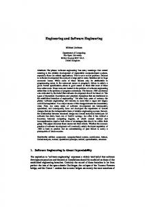
Figures 2.1 Our work builds on top of reverse engineering supported by architecture recovery, software visualization, and software evolution analysis. . . . . . . . . . . . . . . . .
10
3.1 An overview of the Revenge process . . . . . . . . . . . . . . . . . . . . . . . . . . . . . 3.2 Interactive navigation connects the various ecosystem viewpoints . . . . . . . . . . 3.3 When understanding a single system at times one needs to perform architecture recovery . . . . . . . . . . . . . . . . . . . . . . . . . . . . . . . . . . . . . . . . . . . . . . 3.4 The relationships between the elements of the Lightweight Ecosystem Meta-Model 3.5 Three of the subclasses of the Change meta-model element . . . . . . . . . . . . . .
34 37
4.1 4.2 4.3 4.4
47 50 51
4.5 4.6 4.7 4.8 4.9 4.10 4.11 4.12 4.13 4.14 4.15 4.16 4.17 4.18 4.19
Ecosystem exploration pathways . . . . . . . . . . . . . . . . . . . . . . . . . . . . . . . The construction principle of the Size History viewpoint . . . . . . . . . . . . . . . . Size History in REVEAL: the time series represent classes grouped by projects . . . Size History in Gnome: the top view has files grouped by projects; the bottom graph has files grouped by file extensions . . . . . . . . . . . . . . . . . . . . . . . . . The construction principle of the Activity History viewpoint . . . . . . . . . . . . . . Activity History in SCG- the time series represent number of commits per month aggregated to project level . . . . . . . . . . . . . . . . . . . . . . . . . . . . . . . . . . Activity History in Gnome - the time series represent number of commits per month aggregated to project level . . . . . . . . . . . . . . . . . . . . . . . . . . . . . . Activity History in Gnome - time series represent file changes per month grouped by file extension . . . . . . . . . . . . . . . . . . . . . . . . . . . . . . . . . . . . . . . . . The construction principle of the Developer Activity Timeline viewpoint . . . . . . Developer Activity Timeline in REVEAL- the developers are sorted according to their activity similarity . . . . . . . . . . . . . . . . . . . . . . . . . . . . . . . . . . . . . The history of the activity of the more than 900 Gnome developers. . . . . . . . . . The construction principle for the Developer Collaboration viewpoint . . . . . . . . Developer Collaboration in SCG . . . . . . . . . . . . . . . . . . . . . . . . . . . . . . . The construction principle for the Inter-Project Dependency Map viewpoint . . . . Project Dependency Map viewpoint for the SCG ecosystem - color intensity is proportional to the number of commits to the project . . . . . . . . . . . . . . . . . . Inter-Project Dependency Map viewpoint in REVEAL- color intensity is proportional to number of commits to project . . . . . . . . . . . . . . . . . . . . . . . . . . . The construction principle of the Contextual Project Architecture view . . . . . . . The architecture of CodeCrawler . . . . . . . . . . . . . . . . . . . . . . . . . . . . . . . The construction principle of the Contextual Project Dependency Matrix . . . . . .
xv
38 40 43
52 54 55 56 57 59 60 62 63 64 66 68 69 70 71 73
xvi
Figures 4.20 The Contextual Project Dependency Matrix for the CodeCrawler project . . . . . . 4.21 The Contextual Project Dependency Matrix for the SmaCC project . . . . . . . . . .
74 75
5.1 The growth of the code in the Bern ecosystem . . . . . . . . . . . . . . . . . . . . . . 81 5.2 The scatterplot of the projects in the SCG ecosystem. The x-axis represents project size measured in number of classes; the y-axis represents activity measured in number of commits to the version repository . . . . . . . . . . . . . . . . . . . . . . . 82 5.3 Two complementary perspectives on the projects that were active in the last year in the Bern ecosystem . . . . . . . . . . . . . . . . . . . . . . . . . . . . . . . . . . . . . 84 5.4 The distribution of the number of months the developers are active in the SCG ecosystem . . . . . . . . . . . . . . . . . . . . . . . . . . . . . . . . . . . . . . . . . . . . . 85 5.5 The periods when the 120 developers in the SCG ecosystem have been active . . 86 5.6 The top 20 percent developers in terms of number of active months in the ecosystem 87 5.7 The shapes of commit activity of six of the longest contributors to the ecosystem . 88 5.8 Collaboration relationships between the most active subset of developers in the SCG ecosystem . . . . . . . . . . . . . . . . . . . . . . . . . . . . . . . . . . . . . . . . . . 89 5.9 Overview of Moose: the size/activity evolution, the contributors, and topics extracted from code analysis . . . . . . . . . . . . . . . . . . . . . . . . . . . . . . . . . . . 91 5.10 Moose in the context of the ecosystem . . . . . . . . . . . . . . . . . . . . . . . . . . . 92 5.11 The dependency matrix between eight other projects in the SCG ecosystem and Moose . . . . . . . . . . . . . . . . . . . . . . . . . . . . . . . . . . . . . . . . . . . . . . . 93 5.12 The details of the dependency between the ecosystem and MooseModel . . . . . . . 94 5.13 Subclassing between four projects in the ecosystem and Moose . . . . . . . . . . . . 95 5.14 Developer Activity Lines during the last year in the Soops repository . . . . . . . . 97 5.15 At Soops collaboration is abundant . . . . . . . . . . . . . . . . . . . . . . . . . . . . . 98 5.16 Activity Evolution in the Soops Repository between June 2006 and June 2007 with (a) and without Jun (b). . . . . . . . . . . . . . . . . . . . . . . . . . . . . . . . . 99 5.17 Size Evolution in the Soops repository . . . . . . . . . . . . . . . . . . . . . . . . . . . 100 6.1 Reading from left to right the figure presents two successive expand operations. Reading from right to left the figure presents to successive collapse operations. . . 110 6.2 A containment hierarchy of modules where the architectural components are modeled in the modules X, Y and Z. . . . . . . . . . . . . . . . . . . . . . . . . . . . . . 110 6.3 The two types of dependencies between packages . . . . . . . . . . . . . . . . . . . . 112 6.4 a) the color coding. b) the four types of restricted packages; c) an example of the way an extended package is represented . . . . . . . . . . . . . . . . . . . . . . . . . . 113 6.5 The dependencies between between com.aelitis.azureus.core and a working set of the packages in Azureus 2.5.0.4 and the vertical package slice of com.aelitis.azureus.core114 6.6 Possible Configurations for Iceberg packages. a and b are from Azureus while c is a Perfect Iceberg from Infoglue. . . . . . . . . . . . . . . . . . . . . . . . . . . . . . . . 116 6.7 Possible configurations of Fall-Through packages. a) and c) are from Infoglue and b) is from Azureus . . . . . . . . . . . . . . . . . . . . . . . . . . . . . . . . . . . . . . . 117 6.8 Possible configurations of Autonomous packages. Package c) is from jEdit and is also classified as Fall-Through . . . . . . . . . . . . . . . . . . . . . . . . . . . . . . . . 118 6.9 Possible configurations of Archipelago packages. Packages a) and b) display perfect structural symmetry. . . . . . . . . . . . . . . . . . . . . . . . . . . . . . . . . . . . . 119
xvii
Figures
6.10 Softwarenaut exploring the Azureus case study. In the Exploration Perspective the packages are annotated with navigation suggestions . . . . . . . . . . . . . . . . . . 122 7.1 A very high level view of Azureus, generated with Softwarenaut . . . . . . . . . . . 127 7.2 The relationship between Module 1 and Module 2 is the set containing the three aggregated dependencies (D1 , D2 , and D3 ). . . . . . . . . . . . . . . . . . . . . . . . . 128 7.3 The part of the meta-model that supports relationship evolution analysis . . . . . . 130 7.4 The filmstrip principle: time flows from top to bottom, size metrics are mapped on modules and dependencies . . . . . . . . . . . . . . . . . . . . . . . . . . . . . . . . 131 7.5 The evolution of the relation between org.argouml.uml and org.argouml.persistence.132 7.6 A fossil relationship from the ArgoUML case study . . . . . . . . . . . . . . . . . . . . 134 7.7 A lifetime relationships from the ArgoUML case study . . . . . . . . . . . . . . . . . . 136 7.8 An old relation from the ArgoUML case study . . . . . . . . . . . . . . . . . . . . . . . 138 7.9 A recent relation between two modules in the ArgoUML case study . . . . . . . . . 140 7.10 Recent relationships that involve the org.argouml.i18n module. . . . . . . . . . . . 141 7.11 A stable relationship from the Azureus case study . . . . . . . . . . . . . . . . . . . . 142 7.12 An instable relationship from the Azureus case study . . . . . . . . . . . . . . . . . . 144 7.13 All 114 relationships between a set of 23 modules in Azureus 4.2 . . . . . . . . . . 148 7.14 The difference between all the relation in the last version (left) and all the lifetime relations in the system (left) in the Azureus case study . . . . . . . . . . . . . . . . . 148 7.15 Integrating the dependency evolution patterns in Softwarenaut . . . . . . . . . . . . 149 7.16 A screenshot of the Relationship Evolution Pattern Browser during the analysis of ArgoUML . . . . . . . . . . . . . . . . . . . . . . . . . . . . . . . . . . . . . . . . . . . . . 151 A.1 Screenshot presenting the various parts of the UI of Small Project Observatory . . A.2 Two ways of filtering elements in SPO: by composing rules, and by interactively eliminating elements from the viewpoints . . . . . . . . . . . . . . . . . . . . . . . . . A.3 After setting the alias for the user kmaraas and markmc the developer that seemed to be the most active in the Gnome ecoystem, became even more active . . . . . . A.4 Visualizing in SPO an architectural view that was generated in Softwarenaut . . . A.5 The architecture of SPO . . . . . . . . . . . . . . . . . . . . . . . . . . . . . . . . . . . . A.6 A screenshot of Softwarenaut exploring Softwarenaut. Details about the selected dependency are presented in the right panel. . . . . . . . . . . . . . . . . . . . . . . . A.7 The relationship filtering panel in Softwarenaut . . . . . . . . . . . . . . . . . . . . . A.8 The Detailed Project Model can model any hierarchical decomposition of a system written in an object-oriented language . . . . . . . . . . . . . . . . . . . . . . . . . . .
162 163 164 165 166 168 170 172
xviii
Figures
Tables 4.1 An overview of the four ecosystem case studies . . . . . . . . . . . . . . . . . . . . . . 4.2 Average growth rates for four of the ecosystem case studies . . . . . . . . . . . . . .
48 53
6.1 Overview of the six open-source systems used during the package pattern validation experiments . . . . . . . . . . . . . . . . . . . . . . . . . . . . . . . . . . . . . . . . . 115 6.2 The frequency of occurrence of the patterns in the case study systems . . . . . . . . 120 6.3 Pairwise overlapping between the package patterns . . . . . . . . . . . . . . . . . . . 121 7.1 The types of low-level dependencies between elements in an object-oriented system128 7.2 An overview of the Azureus and ArgoUML case studies . . . . . . . . . . . . . . . . . 133 7.3 The frequency of occurence of the dependency patterns in the case studies . . . . 146
xix
xx
Tables
Part I
Prologue
1
Chapter 1
Introduction “In the long run, every program becomes rococo, then rubble” wrote Alan Perlis in 1982 [Per82]. Some years later, David Parnas argued along similar lines that changes to software systems not done in concordance with the initial design of the system lead to the degradation of the architecture, the decrease in quality of the code, and the increase in the maintenance effort [Par94]. Sommerville [Som95] and Davis [Dav95] estimated that the cost of software maintenance is between 50% and 75% of the overall cost of a software system; more recent studies attribute even larger percentages to maintenance [Erl00]. This means that discovering techniques and building tools that ease maintenance can have a strong impact on reducing the total cost of software development. The cost of maintenance is high, because maintenance is a time-consuming activity. Maintainers have to work hard to understand the structure, behavior and effects of the subject system and its relationship to the application domain [BMW94]. Corbi showed in a study that more than half of the time spent on maintenance is dedicated to understanding the system [Cor89]. There are two fundamental causes for the difficulty of program understanding: first, frequently the system’s maintainers are not its developers so they are unaccustomed with the system; second, often the documentation of the software is obsolete or missing [KC98], so the only source of information that is available is the code. For dealing with systems for which code is the only reliable representation, the IEEE-1219 standard recommends reverse engineering as a key supporting technology [IEE98]. Reverse engineering is a process concerned with identifying a system’s components and their interrelationships, and creating representations of the system at a higher level of abstraction [CC90]. Thus, the main goal of reverse engineering is deriving information from the available software artifacts and presenting this information in a way that is easily understandable for the developers and analysts. Over the last decades, reverse engineering research has provided a wide range of methods for analyzing software systems and supporting their understanding. Each of these methods works at one of three levels of granularity: at the lowest level, the methods support the understanding of the source code of a system; at the next level, the methods are concerned with extracting the design of a system; at the highest level, the methods focus on recovering the architecture of a system. In all these cases, the focus of the analysis is an individual system isolated from its context.
3
4 However, software systems are seldom developed and exist in isolation. Instead, they exist in the wider context of an organization or a community, in larger software ecosystems. A software ecosystem consists of the entire collection of software systems developed in an organization. These projects share code, depend on one another, share developers between themselves, reuse the same code, and can be built on similar technologies. For companies with multiple teams of developers working on multiple software projects, the maintenance, understanding, and monitoring of the software ecosystems can be critical. Failing to maintain an accurate and holistic image of the ecosystem can lead to wasted effort and development inefficiencies. Common reasons for such inefficiencies are: • Reimplementing from scratch functionality that could have been reused from other projects in the organization. These projects could have been developed in the past or can be currently undergoing development. • Modifying a component without being aware of all the clients of that component and of the way they use the component. This increases the risk of breaking the code of other people. • Failing to realize the actual structure of the teams and to optimize the collaboration between developers. In order to avoid these and other similar, developers, project managers, software architects, and quality assessment engineers need to be continuously aware of the evolution of the projects and of the social structure that emerges around them: understanding and monitoring an ecosystem means understanding both its social structure and its projects. The main reason for which keeping track of the evolution of the ecosystem is difficult is that there is usually no documentation at the ecosystem level. This means that significant knowledge about the ecosystem exists only in latent form in the social structure of the organization. As the ecosystem grows larger, the chance that any individual will be able to keep track of all its facets decreases. This situation is aggravated in environments with a high turnover where it can be the case that the ecosystem’s maintainers are not its developers. In our case studies, we encountered multiple situations in which no developers are active in an ecosystem from the beginning to the end. Since no documentation exists and no individuals can keep track of all the information, a safe solution is to generate ecosystem documentation based on the available sources of information. Reverse engineering a software ecosystem means recovering high-level views that present aspects that are relevant for the understanding of the ecosystem from existing lower level sources of information. The recovered views need to present both developer-centric and project-centric aspects of the ecosystem. In this context, we formulate our thesis in the following way:
Thesis Visualizing structural and evolutionary information of software projects in the context of their ecosystem supports the reverse engineering of the ecosystem and improves the reverse engineering of the individual projects. In this dissertation we show that visualizing the information stored in the versioning repositories of the projects that are part of the ecosystem, when available, it is valuable for reverse
5 engineering. For this we introduce an ecosystem reverse engineering process we call Revenge. The process is based on analyzing the super-repository associated with an ecosystem. A superrepository is a collection of versioning systems for multiple projects. Super-repositories can be implicit (they are just a collection of versioning repositories for a set of projects) or explicit (they are more than the sum of the parts because they contain information about the relationships between the individual projects that are versioned). Revenge supports the reverse engineering of software ecosystems by automatically recovering high-level views of the ecosystem. It also integrates the individual system reverse engineering in the context of ecosystem reverse engineering in two ways. First, Revenge includes viewpoints which present a system in the context of its ecosystem. Second, since Revenge supports the navigation between the ecosystem granularity level to the system granularity level. There are two types of information that Revenge uses when analyzing an ecosystem: the meta-annotations present in the super-repository, and the source code of the contained projects. Meta-annotations. This information regards both developers and projects and their evolution in the context of the ecosystem. By modeling and analyzing this information we can recover developer- and project-centric viewpoints that highlight the developer collaboration, the inter-project dependencies, the developer activity history, the inter-developer dependencies. Source Code. By analyzing the source code, we can build detailed models of all the individual projects in the ecosystem. The detailed models can be analyzed at different levels of granularity. Since we consider the ecosystem to be the level above the architecture of individual systems, we are mainly interested in analyzing the architecture of the individual systems to support the understanding of the entire ecosystem. Once the information in the super-repository is analyzed, the Revenge process generates visual representations of the ecosystem that capture its various facets: the social structure, the evolution of various metrics in the ecosystem, details about the developers that contribute to the ecosystem, relationships between the composing projects, and views which present a system in the context of the ecosystem. Analyzing an ecosystem is an exploratory task: an analyst interactively navigates and interacts with the generated visual representations. Indeed, the need for interactive visualization is widely recognized by experts in reverse engineering [KC99]. To support the interactive exploration of the proposed viewpoints, in this thesis we introduce tools that are part of our Revenge Toolset. The tools allow the navigation between the various views and the interaction with the individual elements of the views. One particular type of interaction is top-down navigation, in which the analyst dives into architectural views of individual projects in the ecosystem in order to learn more about them. This type of navigation crosses the boundary of two levels of abstraction: the ecosystem level and the single-system, architectural level. The importance of this type of navigation, was anticipated by Müller et al. when they stated that “in the future of software engineering, it is important to understand software at various levels of abstraction and maintain mappings between these levels” [MJS+ 00]. In our case, mapping the levels of abstraction means going from views that present the entire ecosystem to views that present the architecture of the individual projects. Vertical navigation is crucial since during the exploration of the ecosystem questions arise that need to be solved based on low-level information about the individual projects. Examples of such questions are: “What is the reason for the existence of a dependency between two projects?” or “Are there
6
1.1 Contributions
reusable components in this project?”. A general question that we answer in the context of vertical navigation is “Can we learn more about an individual project when we study it in the context of its ecosystem?”. To support vertical navigation, ideally we would automatically generate meaningful architectural views of the system that would present relationships between the main components of the project and present these architectural views in the context of the ecosystem. Since all the existing architecture recovery techniques involve human intervention to various degrees, Revenge assumes a step in which architectural views are recovered from individual systems in the ecosystem. To reduce the amount of human involvement in the process, we introduce two techniques: the first technique automates the discovery of relevant views based on classifying modules in structural patterns, and the second technique automatically filters out relationships based on the goal of the analysis.
1.1
Contributions
The contributions of this dissertation can be classified in three categories: methods and techniques, case studies, and tools. We list them here:
Methods and Techniques • Defining the problem of reverse engineering software ecosystems and presenting the importance of ecosystem analysis. • Providing a methodology for reverse engineering software ecosystems. The methodology, named Revenge, is based on recovering high-level, interactive, views of the ecosystem that correspond to project-centered or developer-centered viewpoints. The methodology emphasizes the importance of connecting the ecosystem granularity level with the singlesystem granularity level in reverse engineering [LLGH07]. • Providing a meta-model for software ecosystems that is independent of the versioning system and programming languages of the contained projects. The model combines information from the analysis of the meta-information of the versioning systems of the projects and the static analysis of the source code of the projects [LGL09]. • A technique for semi-automating the extraction of architectural views from software systems. The technique is based on a classification of inter-module relationships based on their evolution. Recovering architectural views of the projects in the ecosystem is part of the Revenge methodology [LLG06]. • Techniques for analyzing and understanding high-level architectural relationships between modules. To understand an architectural view one needs to understand the relationships between modules in the view. Our approach supports this understanding by studying the evolution of inter-module relationships [LL07].
Case studies • Presenting a set of ecosystems as case studies. The studied ecosystems have a diverse provenance: some are academic, some are industrial, and some are open-source [LLGH07; LML09]. Their size ranges from tens to hundreds of projects and developers.
7
1.2 Structure of the Dissertation
Tools • The Small Project Observatory is an online platform that supports ecosystem reverse engineering through visualization and exploration [LGL09]. We built the tool to validate the ecosystem reverse engineering methodology presented in this thesis. The tool is available online and makes several of the case studies available for study. • Softwarenaut is a tool for software architecture recovery through visualization and exploration [LL06b]. Once the architectural views are obtained in Softwarenaut they can be imported by The Small Project Observatory and used during the vertical navigation process.
1.2
Structure of the Dissertation
Part I: Prologue.
In this part we place our work in the broader context of reverse engineering.
• Chapter 2 (p.9) presents an overview of the related work in reverse engineering. Although there is no work that treats entire ecosystems as first class entities, our work is closely related to architecture recovery, software evolution analysis and software visualization. The chapter surveys the relevant work in the corresponding areas. Part II: Software Ecosystems. In this part we formally introduce the concepts of ecosystem and ecosystem reverse engineering. We present our ecosystem reverse engineering process and multiple case studies that range broadly in scope and size. • Chapter 3 (p.25) introduces the concept of the software ecosystem as another level of abstraction in software analysis. Then it defines Revenge, our process for reverse engineering software ecosystems which is an extension of traditional single-system reverse engineering. • Chapter 4 (p.45) defines a catalog of ecosystem viewpoints. It also introduces a set of ecosystems that we use as case studies. We illustrate the proposed viewpoints with examples from the case study ecosystems. • Chapter 5 (p.79) introduces two case studies of ecosystem analysis. The first ecosystem belongs to the Software Composition Group in Bern. During the case study we show how in some cases analyzing an individual system in the context of the ecosystem can provide supplementary insight into that system. The second belongs to an industrial partner who performed the analysis himself on the company’s ecosystem. Part III: Architecture Recovery. This part addresses challenges that are posed by understanding single systems in the context of an ecosystem. The two main problems are automating the generation of architectural views and understanding inter-module relationships. • Chapter 6 (p.107) presents our semi-automatic approach to generating architectural views of a software system. The approach is based on discovering package patterns. We validate the patterns that we discover on several open-source systems.
8
1.2 Structure of the Dissertation • Chapter 7 (p.125) introduces two complementary ways of analyzing inter-module relationships. The relationship evolution filmstrip presents the evolution over time of a given relationship. The semantic dependency matrix visually summarizes the low-level dependencies that are abstracted in an inter-module relationship.
Part IV: Epilogue. In this part we step back and look at the entire work as a whole and then conclude. • Chapter 8 (p.155) concludes our work by discussing our approach and the lessons we learned. We then present a set of research directions that are opened by this thesis. • Appendix A (p.161) presents the tool support that made all the analysis in the thesis possible. We introduce the architecture and interaction facilities of Softwarenaut, our architecture recovery tool and The Small Project Observatory, our ecosystem visualization platform.
Chapter 2
State of the Art
Ecosystem reverse engineering is a continuation of traditional reverse engineering in two ways. On the one hand, the techniques used in traditional reverse engineering can be used at the higher abstraction level of software ecosystems. On the other hand, the understanding of an ecosystem is not complete unless the individual projects in the ecosystem are understood too, therefore ecosystem reverse engineering is a continuation of single system reverse engineering. In this context, our research is related mainly to three reverse engineering subfields: software visualization, architecture recovery, software evolution. We survey these research domains to identify current limitations of the state of the art from the perspective of our research goals.
9
10
2.1 Introduction
2.1
Introduction
Maintaining individual systems that represent legacy code that was not written with maintenance in mind, strongly requires adequate reverse engineering techniques and tools. Chikofsky and Cross define reverse engineering as: “The process of analyzing a subject system to identify the system’s components and their relationships, and to create representations of the system in another form or at a higher level of abstraction.” [CC90] As the definition points out, reverse engineering has been traditionally done at the level of individual systems. To the best of our knowledge, nobody has attempted before to reverse engineer entire software ecosystems, so there is little direct related work. However, our work reuses existing techniques used in reverse engineering, and draws inspiration from existing reverse engineering processes. Figure 2.1 highlights three main fields of related work: software visualization, architecture recovery, and software evolution analysis.
Ecosystem Reverse Engineering
Software Visualization
Architecture Recovery
Evolution Analysis
Reverse Engineering
Figure 2.1. Our work builds on top of reverse engineering supported by architecture recovery, software visualization, and software evolution analysis.
In this chapter we present in more detail the way our work is related to the three fields: Software Visualization. Visualisation is a powerful mechanism that helps analysts to cope with large amounts of information such as the one available in software ecosystems. Existing research in software visualization addresses various levels of abstraction; from code-level visualization to architectural-level visualizatoin, but no existing research addresses the ecosystem level. Architecture Recovery. Architecture recovery is a highly interactive process which aims at recovering architectural views of a system. The process is not yet fully automated but there is room for improving the process, and the last part of our thesis is concerned with this. Architecture recovery is an inspiration for ecosystem reverse engineering through the concept of viewpoints and through the highly interactive nature of both the processes. Software Evolution Analysis. Software evolution analysis is a research field which has already considered collections of software systems as subjects of study. However, the focus of the research was discovering principles of evolution for individual projects, and therefore the
11
2.2 Software Visualization collection of projects was not studied as an entity in itself as it is the case in ecosystem analysis.
Structure of the Chapter We present the related work in the following order: in Section 2.2 (p.11) software visualizatoin, in Section 2.3 (p.13) architecture recovery, and in Section 2.4 (p.16) evolution analysis. We conclude the chapter with Section 2.5 (p.18) in which we go again through the main observations in the chapter and show how they point to the need for analyzing software ecosystems.
2.2
Software Visualization
Software visualization is a specialization of information visualization in which the focus lies on visualizing software [Lan03b]. Stasko et al. define software visualization as the use of the crafts of typography, graphic design, animation, and cinematography with modern human-computer interaction and computer graphics technology to facilitate both the human understanding and effective use of computer software. [SDBP98] The main goal of software visualization is to address specific questions whose answers are hard to be expressed in plain numbers or in prose. Examples of such questions that are relevant for maintenance and reverse engineering are: How do developers collaborate inside the organization? How are the maintenance activities distributed over the teams? How did the structure of the organization evolve over time? What are the main components of the system and how do they interact with one another? Software visualization is a field with an extensive history. The first taxonomy of software visualization tools was provided by Price et al. in 1993 [PBS93]. One criterion for the classification of software visualization tools is the data that the tool is visualizing. Based on it we distinguish three main classes of visualization tools: 1. Algorithm animation tools are usually didactic, and their goal is to support understanding algorithms [Bae81; RCoP92; BS84]. 2. Dynamic visualization tools present information that is derived from instrumenting the execution of the program [DPHKV93; DPJM+ 02; LN97]. Their goal is to support understanding the behavior of the systems. 3. Static visualization tools visualize information extracted by static analysis of the software [MK88; SM95; Lan03a]. Their goal is to support the understanding of the structure of the system. Our work is focused on static visualization tools. These tools exist and work at several levels of abstraction. The following classification is based on the types of elements that are visualized at each abstraction level: lines of code for the code level, classes and files for the design level, and modules and their relationships for the architectural level. Code-Level Visualization. The most basic software visualization techniques are code formatting and pretty printing. Introduced in the 70s for Lisp in simpler form, the pretty printers are today integrated in all modern IDEs.
12
2.2 Software Visualization Even when displaying code-level information, visualization is most useful when larger amounts of information need to be displayed. Eick et al. used a code line to pixel line mapping for representing the files in a software system [ESJ92]. On top of this mapping, they superimposed other types of information such as where functions are called or which developer worked on a given line of code. Later, Ducasse et al. used a character-to-pixel representation of methods in object-oriented systems enriched with semantical information to provide overviews of the methods in a system[DLR05].
Design-Level Visualization. At a higher level of abstraction, Lanza and Ducasse introduced the class blueprint [DL05] which provides a call-flow based representation of classes. Class blueprints are enriched with semantical information extracted from control flow analysis. UML diagrams are the industry standard for representing object-oriented design and there are many tools that provide support for recovering UML diagrams from code (e.g., Rational Rose, ArgoUML, Enterprise Architect). However, UML is not targeted specifically for reverse engineering [DDT99]. One of its main drawbacks is the lack of scalability. Termeer et al. address the overview problem in their tool MetricView by augmenting UML diagrams with visual representations of class metrics [TLTC05]. Lanza addressed the scalability problem with polymetric views, a lightweight software visualization technique enriched with software metrics information [LD03; Lan03b]. A wellknown polymetric view, the System Complexity presents the class hierarchy of a system where classes are represented as rectangles with three distinct metrics mapped on their width, height and fill color intensity. Such a representation is more scalable than a UML diagram, and can be used as a first step in the reverse engineering process. Metrics are especially appropriate for presenting high-level overviews and supporting the detection of outliers. A special class of visualization tools that combine structural and metric visualization is 3D visualization tools. Marcus, Fend and Maletic propose in their sv3D, a 3D representation of software systems inspired by Eick’s SeeSoft [MFM03]. Wettel and Lanza argue that a city is an appropriate metaphor for the visual representation of software systems and implement it in their CodeCity tool [WL07]. Some tools focus on visualizing the evolution of the relationships between classes in an object-oriented system. For example, Collberg [CKN+ 03], focus on providing intelligent and fast layout algorithms that present the evolution of the relationships between classes and scales to very large systems. Architectural-Level Visualization. One of the most common ways of specifying architecture is to visualize the modules and the relationships in a system. The first architectural visualization prototype was Rigi, a programmable reverse engineering environment which emphasizes visualization and interaction [MK88]. Rigi can visualize the data as hierarchical typed graphs and provides a Tcl interpreter for manipulating the graph data. The reconstruction process is based on a bottom-up process of grouping the software elements into clusters by manually selecting the nodes and collapsing them. Rigi also offers various capabilities for filtering the nodes, navigating the hierarchical models and making layouts. Rigi comprises both an extraction component and a user interface component. Other architecture visualization tools were built on top of Rigi [KC98; OS01].
13
2.3 Architecture Recovery One of the projects that was inspired by Rigi was the SHriMP tool [SM95] and its Eclipsebased continuation, Creole [LMSW03]. SHriMP and Creole display architectural diagrams using nested graphs. Their user interface embeds source code inside the graph nodes and integrates a hypertext metaphor for following low-level dependencies with animated panning, zooming, and fisheye-view actions for viewing high-level structures.
2.3
Architecture Recovery
Understanding the architecture of a large software system is a prerequisite for its maintenance and development. Two problems make architecture understanding difficult: architecture is usually not explicitly represented in the code, and architecture is the subject of degradation, drift, and erosion [PW92]. Jazayeri et al. defined architecture recovery as “the techniques and processes used to uncover a system’s architecture from available information”[JRvdL00a]. Before defining architecture recovery one needs a definition of software architecture, of which there are many definitions each one with a slightly different perspective. In this thesis we use the one provided by Bass and Clemens according to whom software architecture is the structure or structures of the system, which comprise software elements, the externally visible properties of those elements, and the relationships among them [BCK97]. This definition is similar to the one proposed by the IEEE 1471 standard [14700], in that they both emphasize elements and the relationships between them. In large software systems, the architecture is specified through multiple architectural views. An architectural view is a representation of a whole system or of part of a system from the perspective of a related set of concerns. Each architectural view conforms to a viewpoint. A viewpoint is a pattern or template from which to develop individual views by establishing the purposes and audience for a view and the techniques for its creation and analysis [14700]. Although different authors propose different viewpoints [BCK97; Kru95; HNS00] there are two points of consensus. First, all the proponents agree that the architecture of a system is complex and multifaceted and that multiple viewpoints are needed to express it. Second, all the authors specify one viewpoint which presents the modules and the static relationships between them. Bass and Clemens call this viewpoint the module viewpoint. Most of the work in architecture recovery is focused on recovering views that correspond to the module viewpoint.
Architecture Recovery Tools The majority of the architecture recovery techniques are based on the extract-abstract-view process model [TSP96]. In such a process, data about source code artifacts is extracted from a software repository. Using analysis techniques, this data is abstracted to a higher level. The abstracted data is then presented by appropriate visualization means. The model extraction step is done by specialized tools that are called parsers or fact extractors, that can either be stand-alone like the ANTLR parser generator, or part of larger analysis frameworks like iPlasma [MMMW05] and Columbus CAN [FBTG02]. To allow the interoperability of the extractors and other tools the results of the extraction phase are usually exported in an intermediate format such as RSF [Won98], GXL [HWS00] or MSE [DGLD05]. Some architecture recovery techniques focus on the abstraction and analysis step, some focus on the visualization step and yet others provide a common integration framework. Two of the
14
2.3 Architecture Recovery
classical architecture recovery platforms that focus on providing a common integration platform are Dali and The Software Bookshelf. Both platforms are focused on providing an integration framework for multiple individual tools: Dali is a workbench focused on easing the interaction between various extraction, manipulation, analysis, and presentation tools [KC98; KC99; WCK99]. The various tools interoperate through a shared database. One of the cornerstone ideas of Dali is the fusion of views which lets a user combine elements from multiple views together. The Software Bookshelf is a framework for capturing, organizing, and managing information about a system’s software [FHK+ 97]. The Bookshelf framework is an open architecture that allows many reverse engineering tools to be integrated. Reverse engineering tools can populate the Bookshelf and other tools can retrieve this information.
Architecture Recovery Processes Over the years, researchers have proposed multiple theories of program comprehension. One of the oldest theories argues that the developers use a bottom-up comprehension process in which they read the code and as they read, they integrate the information and form higher level mental models [Shn80]. An opposite theory argues that comprehension happens in a top-down fashion and the developers first generate a high-level hypothesis about the code, and then proceed to verify that hypothesis [Bro83; SE86]. Von Mayrhauser and Vans proposed an integrated model in which programmers use both the processes and alternate between them[vMV95]. Letovsky proposed a similar model in which he sees the programmers capable of exploiting either topdown, or bottom-up approaches in the process of building the mental model of the program [Let86]. Although none conforms exclusively to a single theory, the majority of the architecture processes fall in two main classes, corresponding to whether they are dominantly assuming a topdown or a bottom-up comprehension.
Top-down Processes Top-down processes start with high-level knowledge such as requirements or architectural styles and aim to discover architecture by formulating conceptual hypotheses and by matching them to the source code [Bro83; SFM99]. A few examples of top-down processes can be found in literature: • In 1999, Bowman, Holt and Brewster performed one of the most well-known case studies of architecture recovery, by extracting the architecture of the Linux kernel [BHB99]. They began their study by forming the conceptual architecture of the Linux kernel. The conceptual architecture, or the as-designed architecture, shows how the developers are thinking about the system in terms of components and relationships between them. Then, they extracted the concrete architecture. The concrete architecture, or the as-is architecture shows the relations that exist in the implemented system. By comparing the conceptual and the concrete architecture, they discovered multiple occurrences of divergences between the two types of architecture - especially at the relationship level. • The idea of comparing the two types of architecture, was introduced earlier by Murphy and Notkin in their reflexion modelling work [MN95; MNS95]. The reflexion models approach uses a regular expression mechanism for specifying components of the conceptual
15
2.3 Architecture Recovery architecture and a lightweight, robust source model extraction tool for inferring a wide array of relationships among the components of the concrete architecture. • Christl et al. presented an evolution of the reflexion models [CKS05]. They enhance it with automated clustering to facilitate the mapping phase. As in the reflexion models, the reverse engineer defines his hypothesized view of the architecture in a top-down process. However, instead of manually mapping hypothetic entities to concrete ones, the new method introduces clustering analysis to partially automate this step. • Other researchers have proposed similar approaches, which differ mainly in the way the rules for specifying the conceptual architecture are defined. Mens et al. proposed another variant of architecture conformance checking with their Intensional Views [MKPW06]. They use rules specified in Prolog to encode external constraints that are checked against the actual source code. Recently Bruehlmann et al. use annotations to specify the mapping between the software modules and the architectural layers of a system [BGGN08].
As we can see from the examples, these approaches tend to be geared towards verifying the conformity of an architecture about which one has previous knowledge.
Bottom-up Processes Bottom-up processes start with low-level knowledge about the system (such as the code), and they progressively reduce these facts by filtering and abstraction until a high-level model of the system is reached. • The traditional tool that supports a bottom-up architecture recovery process is Muller’s Rigi [MK88]. In Rigi, the user starts with a view which contains all the artifacts in the system and refines the view by grouping elements together in higher-level abstractions, and therefore, reducing its complexity. During the exploration, the user generates various views which are representative for the architecture of the system. • Krikhaar proposed the SAR (Software Architecture Reconstruction) technique for creating abstracted, high-level views of the architecture of a software intensive system [Kri99]. The process of abstraction in SAR is based on relational partition algebra, an extension of relational algebra introduced by Feij et al. that supports a formal description of software architectures [FKO98]. • Riva proposed NIMETA, a view-based architecture reconstruction approach which is based on the relational algebra [Riv04]. NIMETA emphasizes the selection of architectural concepts and architecturally significant views that are reflecting the interests of the stakeholders. • Pinzger proposed the ArchView approach [Pin05] which is similar to SAR but augments the analysis and visualization with information about the evolution of the modules in a system. His evolution analysis takes into account the annotations from the versioning system repository. ArchView proposes two types of views that summarize the extracted architectural information: visualizations of multiple evolution metrics with Kiviat diagrams and polymetric views.
16
2.4 Software Evolution Analysis
Bottom-up processes are more adequate for discovering the de facto architecture of a system since they do not require a priori knowledge about the system. For this type of processes interaction and support for exploratory analysis is critical [Riv04; KC99]. About the classical bottom-up Dali, Kazman et al. declare that “probably the most important component of the Dali workbench is the interaction element” (Kazman, 1999).
Commonalities between the two processes There are two factors that unite the two previous architecture recovery processes: 1. The majority use multiple views to capture different aspects of the subject system’s architecture. The different views can correspond to the same viewpoint like in the case of Bowman et al. [BHB99] or present different viewpoints like in the case of Pinzger [Pin05]. 2. They all involve the user playing an active exploratory role in the process. The user’s tasks vary based on the starting state of the exploration process, and the operations that he has at his disposition: • In some processes the user starts the exploration with a view which contains all the artifacts in the system. He then proceeds to refine the view by filtering and grouping elements in the view. This is the case with most of the approaches based on Rigi [MK88; OS01; KC99; Riv04]. • In some processes the user starts the exploration from a very high-level view of the system. He then explores the architectural information by bringing information into the view as needed. This type of navigation is the dominant interaction in SHriMP and its Eclipse-based follow-up, Creole [SM95; LMSW03] as well as in our prototype Softwarenaut [LKGL05]. • In some processes the user starts with a blank visualization. He then proceeds to add elements as he explores and discovers the system. Janzen and De Volder use this approach in JQuery [JV03] and Sinha et al. use this approach in Relo [SKM06]. Even if there are no fully automatic techniques, there is still a need for increasing the amount of automation of the processes and decreasing the human involvement.
2.4
Software Evolution Analysis
In recent years considerable research effort has been directed towards understanding software evolution. The basis for the work is the widespread use of versioning control systems and the availability of open-source case studies. There are two main research directions when studying system evolution: discovering general principles of software evolution, and supporting program understanding and maintenance. We elaborate on the main directions here.
Discovering general principles In 1985 Lehman proposed a number of “laws of software evolution” [LB85; LPR+ 97]. The laws are based on metrics collected by observing the evolution of multiple industrial systems
17
2.4 Software Evolution Analysis
over many years. The principles are very general. For example, the principle of continuing change postulates that systems must be continually adapted else they become progressively less satisfactory. Given the large variability in the environments, technologies and processes for software development, it is not surprising that overarching, more specific principles are hard to find. When attempting to understand the fundamentals of the evolution of software systems researchers need to investigate large groups of projects. They analyze these projects in parallel, but they rarely look at the entire group of projects as the subject of the analysis. One such example is the analysis of all the projects on SourceForge by Weiss [Wei05]. The Libresoft research group in Spain has investigated in several occasions entire collections of software projects. In one instance, they analyzed the Debian Linux distribution and estimated the cost of implementing it from scratch [ARGBH05]. In another article, they proposed a methodology for analyzing how the developer turnover affects open-source software projects by taking several representative open-source projects and analyzing the information in their versioning system repositories [RGB06]. In yet another case they studied from a social networking point of view the developers that are working in the Apache and Gnome projects [LFRGBH06]. One project that does not perform evolution analysis per se, but is rather an enabler for this type of analysis is FlossMole [CHC05]. The project compiles every two months a database with statistics about a very large number of open-source projects. The database includes projects from SourceForge, Freshmeat, RubyForge and a few other public project repositories.
Supporting Program Understanding and Maintenance Since the versioning repository of a software project is a rich source of information, it is natural that researchers attempt to use this information to support the development and maintenance processes. The existing research in this direction analyzes the evolution of individual systems focusing on different goals: • Focus on predicting the locations of future changes. Sahraoui et al. studied the interfaces of classes in libraries written in object-oriented systems in order to predict the future stability of their interfaces [SBLE00]. Gîrba et al. used historical information about a system to suggest starting points for the reverse engineering process based on the assumption that those parts of the system that changed recently are the ones who need to be understood first [GDL04]. In a related work, Zimmerman et al. showed that the parts of the system that have changed together in the past are likely to change togehter in the future [ZWDZ04]. Recently Robbes proposed an approach in which he keeps track of every individual change that is collected through the IDE to allow for a more fine grained analysis of the changes [Rob08]. • Focus on increasing the quality of IDE support during forward engineering. Cubranic et al. have proposed using project information to support the automatic recommendation of the parts of the system which are involved in a maintenance task [CMSB05]. In their case, project information comprises a number of different sources, including the source code versions, modification task reports, newsgroup messages, email messages, and documentation. Kersten suggested program elements that are likely to be related to the task at hand based on a degree of interest model built from the history of the navigation in the IDE [KM05]. Singer et al. proposed NavTracks a tool that keeps track of the navigation
18
2.5 Towards Reverse Engineering Software Ecosystems history of software developers, forming associations between related files. These associations are then used as the basis for recommending potentially related files as a developer navigates the software system [SES05]. • Focus on supporting program understanding. The work that uses evolutionary information in the context of program understanding and reverse engineering has a strong visualization component. Collberg studied the evolution of the structure of software systems from the graph drawing optimization perspective [CKN+ 03]. He introduced a scalable way of visualizing large evolving graph structures that represent classes in a software system. Lanza visualized the system’s history in a matrix in which each row is the history of a class. A cell in the Evolution Matrix represents a class and the dimensions of the cell are given by evolutionary measurements [Lan01]. The analysis of a large number of classes led to a classification of classes based on their evolution patterns [Lan03b]. Gîrba et al. took the study of the class evolution one step further in his analysis of the evolution of the class hierarchies [GLD05]. Holt and Pak developed the GASE tool to visualize the evolution of software architecture in the large [HP96]. In their approach they present a visual diff between two representations of the high-levels structure of the system uses colors to contrast new, common and deleted parts of a software system. A similar and more recent work is Motive, a visualization of the evolution of the architecture of the system that enables the user to view the effects of a set of modification records on the architecture of a system [MGWJ07]. The authors argued that visualizing the evolution of a system during a predefined standard interval - e.g. six months, is not enough and architecture evolution visualization tools should visualize the impact of any modification request. • Focus on assessing code quality. In an analysis based on the information in the versioning system, Gall et al. proposed retrospective analysis as a way of assessing the stability of the system. They introduced visualizations that characterize the evolution of a module [GJR99]. Nagappan et al. used historical information about the system to predict the parts of the system which are going to be affected by failures [NBZ06]. Neuhaus used evolutionary information about the system to predict parts of the system which are likely to have vulnerabilities [NZHZ07].
One common characteristic of many of the approaches is the use of metrics. Pinzger studied the evolution of the architecture of a system by visualizing and analyzing evolution metrics for the system’s modules and their relationships [Pin05; PGFL05]. Lanza uses metrics in his evolution matrix to visually depict the evolutionary dynamics of the classes in the system [Lan01].
2.5
Towards Reverse Engineering Software Ecosystems
In this chapter we presented the state of the art in software visualization, evolution analysis, and architecture recovery. Here we reiterate the main observations regarding the three fields that are of interest to our work: • Static software visualization techniques work at several levels of abstraction that range from the code up to architecture. Although there are many software visualization tools, none attempts to support software understanding at a level above architecture.
19
2.5 Towards Reverse Engineering Software Ecosystems • Architecture recovery is an interactive process that requires a human analyst in the loop. Even if there are no fully automatic architecture recovery processes, there is a need for increasing the automated part. • Although most of the work in software evolution analysis is focused on understanding individual systems and supporting their maintenance, there are cases of analysis in which people study entire groups of projects together. In these cases the goal is not building tools that would enhance the maintenance but rather discovering general laws of software evolution.
From the work we have presented we can derive a few constraints for ecosystem reverse engineering: • Multiple Viewpoints. Due to the inherent complexity of large software systems, their architecture cannot be captured in a single view. Instead, multiple viewpoints capture various aspects of a system’s architecture. Given that software ecosystems are even more complex than individual systems, the concept of viewpoint will be useful in their analysis too. • Support for Exploration. Different architecture recovery techniques involve the user in the process in different degrees and none is completely automated. They all involve the user playing an active exploratory role in the exploration process. Ecosystem reverse engineering will also need to support an exploratory analysis. • Navigation Between Levels of Abstraction. One special type of navigation will be navigating between the ecosystem and the single system abstraction level. This will support understanding the importance of individual projects in the wider context of the ecosystem. Since in our view, the abstraction level below the ecosystem is the architecture of a single system, we dedicate our attention to bridging the two levels. In the remainder of this thesis we present the way our ecosystem reverse engineering technique integrates with traditional reverse engineering and architecture recovery and how it uses software visualization and evolution analysis in the process.
20
2.5 Towards Reverse Engineering Software Ecosystems
Part II
Ecosystems
21
Software ecosystems are another level of abstraction at which analysis of software can be performed. One type of analysis is reverse engineering an ecosystem, a process which analyzes lowlevel information about the component projects of the ecosystem and generates high-level views that characterize the ecosystem, its component projects, and the social structure that emerges around them. In this part we introduce Revenge, our ecosystem reverse engineering methodology. Revenge classifies the many possible visual perspectives on an ecosystem into viewpoints. We introduce a catalog of ecosystem viewpoints and exemplify them on various academic, industrial, and open-source ecosystem case studies. To validate the methodology we apply it to two case studies of ecosystem analysis. The first ecosystem belongs to the Software Composition Group in Bern. During the case study we show how in some cases analyzing an individual system in the context of the ecosystem can be useful to both the developers of the system and to clients that depend on that system. The second ecosystem belongs to an industrial partner who performed the analysis himself on the company’s ecosystem.
23
24
Chapter 3
Reverse Engineering Software Ecosystems
Software ecosystems are collections of projects that represent important assets of organizations. Understanding the legacy of code that exists in an ecosystem can support a more efficient allocation of resources and can promote reuse. Since no single person can keep track of the large and diverse amount of information that regards an ecosystem, and since there usually is no documentation for the ecosystem, we need to reverse engineer the ecosystem by extracting useful information about it from the available sources of information such as the source code of the projects or the associated super-repository. In this chapter we introduce Revenge, our ecosystem reverse engineering process. The process has multiple steps, one of which is architecture recovery. Several of the steps involve interactive analysis and exploration. The exploration happens in two dimensions: horizontal exploration allows the navigation between various ecosystem viewpoints; vertical exploration allows diving into the details of the architecture of an individual project. The methodology relies on the Lightweight Ecosystem Model, a representation of an ecosystem which is independent of the super-repository and the programming language used for the development of the projects in the ecosystem.
25
26
3.1 Introduction
3.1
Introduction
No project is an island. Software projects exist in larger contexts that we call ecosystems. Organizations with multiple teams of developers working on multiple software projects are vulnerable to inefficiencies and problems. Scenarios that illustrate this are the following: • Modifications applied to a component without awareness of all its clients and of the way they use the component lead to future integrations problems. • Failing to identify previous projects that already implemented a certain functionality leads to a waste of resources, as the developers reimplement the functionality. • Failing to realize the actual structure of the teams and to optimize the collaboration between developers results in the inefficient allocation of human resources. To avoid these problems, the developers, the managers, and the architects need to be aware of the legacy of source code, the relationships between the projects, and the social structure that emerges in an ecosystem. This type of information is rarely documented at the ecosystem level. Organization charts might exist that present the structure of the organization, but they fail to capture the continuously shifting dynamics of developer collaboration. Dependencies between projects might be documented, but they fail to capture the detailed reasons for the dependencies. In many organizations these documents are missing altogether. The insufficient documentation can be complemented with the knowledge acquired from the contributors to the ecosystem. Nevertheless, there are problems with relying on individuals for providing information about the ecosystem: • Sooner or later the contributors leave the ecosystem. Since an ecosystem can exist independently of every one of its individual contributors, it is often the case that no individual developer contributes for all the ecosystem lifetime. As a result, no individual has all the knowledge about the ecosystem. • Given the large amount of data associated with an ecosystem, not even the most experienced contributor in the organization can keep track of all the aspects of ecosystem evolution. And if there were such an experienced contributor, it would be unreasonable to expect that every time a newcomer has a question about the ecosystem he refers it to him. The goal of ecosystem reverse engineering is to document an ecosystem by extracting information about the associated social structure and the contained project structure from the available sources of information. In this way, ecosystem reverse engineering increases the overall visibility and comprehensibility of the different facets of an ecosystem.
Structure of the Chapter In Section 3.2 (p.27) we define two key concepts of our work: software ecosystems and superrepositories. We then proceed to position the concept of a software ecosystem with respect to other similar concepts in Section 3.3 (p.29). We present who is interested in analyzing ecosystems in Section 3.4 (p.31). In Section 3.5 (p.32) we define ecosystem reverse engineering and in Section 3.6 (p.34) we introduce Revenge, our ecosystem reverse engineering process. In Section 3.7 (p.39) we introduce the ecosystem meta-model that Revenge is based on. In Section 3.8 (p.41) we discuss our approach and we conclude in Section 3.9 (p.43).
27
3.2 Ecosystems and Super-Repositories
3.2
Ecosystems and Super-Repositories
The term ecosystem comes from biology, and according to Webster’s dictionary, it represents the complex of a community of organisms and its environment functioning as an ecological unit. The organisms in a biological environment interact with one another, depend on one another and influence one another. In biology studying an organism in the context of the whole ecosystem can provide valuable information that otherwise would not be observable. At the same time, in order to understand the whole ecosystem, one needs to be able to understand the individuals and their interactions. In our thesis we argue that software systems are part of larger systems that we call software ecosystems. We define a software ecosystem as follows: A software ecosystem is a collection of software projects which are developed and which co-evolve together in the same environment. The environment can be physical, like in the case of a company or a research group that has a geo-spatial identity, but can also be virtual, like the projects that are part of an open-source community. In our studies we have identified three types of environments that can host software ecosystems: • Companies. For a software company, the source code of its projects represents one of its most valuable assets. Often companies that have multiple clients offer them variants of the same product, and their ecosystem becomes populated with duplicated code that needs to be managed. In the same time, the companies buy off-the-shelf frameworks or obtain open-source software that they reuse to build their systems. Companies also develop tools for internal use, or libraries that are used across projects. • Research groups. Research groups, especially in the systems domain, maintain ecosystems of projects built by students and researchers. One characteristic of the ecosystems that are hosted in an academic environment is that they have a high developer turnover since when the students finish their studies they leave the group. This results in the ecosystem accumulating orphan projects that might contain reusable code. • Open-source communities. The open-source software movement has enabled people from all over the world to collaborate on projects around similar philosophies or goals. Two such examples are the Gnome desktop suite1 and the ecosystem of projects managed by the Apache Software Foundation2 . One characteristic of the open-source software ecosystems is the availability for reuse of the source code of the existing projects [Ray99]. However, together with this availability comes the problem of finding the right project to reuse. Each of these environments has an associated social context which emerges as a result of the collaboration between the different contributors to the projects in the ecosystem. Indeed, inside an ecosystem developers collaborate on projects, depend on the code of each other, and share programming patterns and idioms. Each software ecosystem is characterized by its associated social structure. 1 2
http://www.gnome.org/ http://www.apache.org/
28
3.2 Ecosystems and Super-Repositories
Some of the projects are developed inside the ecosystem from the beginning and co-evolve together while others are imported from other ecosystems (e.g., third party libraries, off-theshelf frameworks). If the imported projects start evolving along with the projects that were in the ecosystem from the beginning, they become part of the ecosystem. Since reuse is an important principle in software engineering, in an ecosystem it is likely that the projects will depend on one another, and reuse parts of code between themselves. Customarily, the history of every project in the ecosystem is recorded in the versioning control system of that project. At the ecosystem level we say that the history of the entire ecosystem is recorded in a super-repository. We define a super-repository in the following way: A super-repository is a collection of all the version control repositories for multiple software projects. The super-repository is therefore the technology behind the ecosystem concept. We distinguish between two types of super-repositories: Explicit super-repositories. This type of repository allows for versioning multiple projects in parallel. The project is a first-class entity in an explicit super-repository and this allows for recording extra meta-data about the relationships between projects. Examples of explicit super-repositories are Store and SqueakSource for projects written in VisualWorks Smalltalk or Squeak. In our work we looked at multiple case studies of explicit superrepositories based on Store. Store is a version control system dedicated to versioning systems implemented in VisualWorks Smalltalk [Cin00]. Implicit super-repositories. In this type of repository the existence of a super-repository of projects is merely a convention. For example, in SVN the versions of all the projects are kept in parallel in a common directory on the server, however, there is no explicit concept of an ecosystem. Three of the most frequently used versioning systems that are usually associated with implicit super-repositories are SVN, CVS, and Git [RL05; BRB+ 09]. Super-repositories are a rich source of information about an ecosystem. They contain information about the developers in the form of annotations associated with the versioning system operations. They also contain the various versions of the source code of the projects that are useful in studying the evolution of the individual projects as well as the evolution as a whole. Some super-repositories contain meta-information about project configurations and project dependencies. There are three possible relationships between an ecosystem and a super-repository: 1. The ecosystem includes multiple super-repositories. This is the case when an organization has multiple super-repositories. In our case studies, the Lugano ecosystem contains a Store super-repository for Smalltalk projects and a SVN repository for the Java projects. 2. The ecosystem has exactly one super-repository. This is the case in our Gnome case study where all the projects are versioned in the same logical SVN super-repository. 3. Multiple ecosystems share a single super-repository. This is the case with public superrepositories such as SourceForge, CodeHaus, and GoogleCode, which are so large that several organizations can host all their projects inside them. In our work we focused our attention on the first two cases since they were the only types of ecosystems that we encountered in our case studies.
29
3.3
3.3 Related Concepts
Related Concepts
Project portfolios, product families, collections of unrelated projects, large individual systems, and software distributions, are similar in some aspects to ecosystems. In this section we clarify the similitudes, differences, and relationships between these concepts and software ecosystems.
Project Portfolios Project portfolio management is a term used by project managers and project management organizations to describe methods for analyzing and collectively managing a group of current or proposed projects based on numerous key characteristics. The fundamental objective of project portfolio management is to determine the optimal mix and sequencing of proposed projects to best achieve the overall goals of the organization - typically expressed in terms of hard economic measures, business strategy goals, or technical strategy goals - while honoring constraints imposed by management or external real-world factors. Typical attributes of projects being analyzed in a project portfolio management process include the total expected cost of each project, consumption of scarce human or material resources, expected timeline and schedule of investment, expected nature, magnitude and timing of benefits to be realized, and relationship or inter-dependencies with other projects in the portfolio. The goal of project portfolio management is therefore to optimize the revenue of the company. Our goal is to support program understanding and to increase the awareness of the interactions between the developers and the projects in an ecosystem. The different goals result in different methods. In our approach, interactive visualization, static analysis, and integration with the lower-level levels are preeminent.
Product Families Product family engineering is a method that creates an underlying architecture for the product platform of an organization [JRvdL00b]. It provides an architecture that is based on commonality as well as planned variabilities. The various product variants can be derived from the basic product family, which creates the opportunity to reuse and diversify the products in the family. Product family engineering focuses on the process of engineering new software products in a way which allows reusing product components and applying variability with decreased costs and time. Product family engineering is about reusing components and structures as much as possible. Although product families are collections of projects and ecosystems are also collections of projects, the ecosystem concept is more general. In fact, a product family can be considered as a special case of ecosystem. It is an ecosystem in which all the projects share an underlying architecture. It is possible that some of the techniques that we apply on ecosystem analysis can be used with product families. However, it is likely that inside the organization that owns it, the product family is part of a larger software ecosystem. Like in the case of project portfolio management, the main difference with respect to ecosystems is the goal of the analysis: in one case the goal is understanding, in the other it is extracting and reusing the common architectural components of multiple projects.
30
3.3 Related Concepts
Collections of Unrelated Projects Random collections of projects are similar only since they are larger aggregations of projects but they lack the organizational context of the software ecosystems. One existing application for the analysis of unrelated collections of projects is code search. Code search engines, such as Krugle (krugle.com), Google (codesearch.google.com), and Koders (koders.com) index a large number of open source software projects, written in multiple languages. Academic research has also been directed towards supporting code search with projects that perform keyword-based search [BNL+ 06] or other semantics-based approaches [Rei09]. The goal of the code search engines is to encourage reuse by supporting the discovery of similar code [kru09]. A company or an organization which owns an ecosystem would indeed benefit from being able to search its codebase. One possible application of analyzing a semi-random group of projects is building a benchmark for design and quality assessment. One would create a set of projects that are representative for a given programming language or for a given technology, and then collect metrics about the systems in the benchmark. These metrics would then be used to assess new systems. The idea can also be applied inside an ecosystem.
Individual Systems One question we still need to address is: “what is the difference between ecosystems and very large individual systems?”. Both ecosystems and systems are containers of code, and if a system is large enough, there can be a very large number of developers contributing to it. The first difference is that the goals of the analysis are different. Since an ecosystem contains multiple systems, the problems that are associated with ecosystems are distinct from the ones associated with individual systems. Nevertheless, we show later that ecosystem level analysis represents an entry-point for single system analysis. The second difference is that a project is a unit of release. This results in dependencies between projects and dependencies between modules inside a project being qualitatively different. When a project depends on another project it depends on a certain version of the second; when a module depends on another, the dependency does not involve any explicit versions of the two. One effect of this is that the inter-project dependency graph is less cluttered than the intra-project dependency graph. The third difference is that a project is a unit of deployment (frameworks can be considered as exceptions) whereas an ecosystem is not deployable, nor runnable itself. This limits the type of analysis that one can perform on an ecosystem. For example dynamic analysis and performance optimisation, which are important in the context of an individual system, are meaningless in the context of an ecosystem.
Software Distributions Linux distributions are probably the most complex software ecosystems that currently exist. Built around the Linux kernel such distributions collect together applications that interact with each other. However, there is no central coordination and there are no common goals for the teams. These applications are subject to complex dependency graphs between themselves. A distribution needs a large number of volunteers that manage the dependencies between the projects. One of the most well-known distributions is Debian which was studied by Barahona et al. [GBRM+ 08].
31
3.4 Benefits of Ecosystem Analysis
One of the main differences between Linux ecosystems and our concept of software ecosystems is the fact that a distribution can be considered to be an individual executable system with the individual applications and libraries playing the role of subsystems. As such, it is indeed a particular case of a software ecosystem. However, the collection of projects that belong to a company are rarely being part of an overarching system that uses all of them.
3.4
Benefits of Ecosystem Analysis
Different categories of stakeholders are interested in different aspects of the structure and evolution of an ecosystem. This is a result of the different stakeholders having different relationships with the ecosystem. Here we present some of the different reasons for studying ecosystems of several types of stakeholders: project managers, developers, software architects, and assessment specialists. Project managers are interested in how teams work, how projects evolve, and how to allocate resources to the projects. They need to locate developers with expertise in specific domains. Organizational charts only show the team structure in a static, and often poorly maintained, form. Revealing the activity and collaboration of developers and the projects they work on, shows how the actual work is being performed [GKSD05] and how the collaborations between developers evolved over time. Moreover, since in general successful projects need to continuously change [Leh80; LPR+ 97], a project manager needs to be up to date with how projects change and what their current status is. Developers know about the code they write, and have an idea about the parts of the project that they are working on, but are usually not aware of the overall picture of the ecosystem. An important source of information for developers, especially for newcomers to a project, are other developers. Thus, developers need to know whom to ask various questions to [CMSB05]. When an application is built out of components, developers need to know what components have changed. Developers might know the details of their particular project, but not be aware of the relationship of that project with other projects. For example, the first time a developer begins using a framework he would benefit from knowing how are the other projects that use that framework and how, what are best practice patterns, what are the important classes, etc. For the developers of the framework it would be useful to know how are the clients of the framework using it so they consider the usage information as they evolve the framework. In the open-source context there are also developers looking for interesting projects they can contribute to. Since not all of them have equal chances of success, for a potential contributor it would be useful to gain insights into the evolution of the code, and the social structure of a particular project. Software architects are interested in analyzing past projects to understand the impact of architectural decisions and finding components that can be reused between projects.
32
3.5 Reverse Engineering Software Ecosystems They need to keep track of the existing reusable components and identify projects and components that incorporate functionality of interest.
The quality assessment team is interested in continuously supervising the ecosystem to insure that the quality of the projects in it remains high. They are interested in collecting metrics about projects. It is known that programming languages and methodologies are factors that have a strong impact on software metrics [Mar02]. Extending the metric collection process to the ecosystem allows for the definition of quality thresholds tuned for the specific needs of the organization. One potential application of interest for the quality assessment team is detecting interproject code duplication. Code duplication inside a project is easy to detect because developers who collaborate on that project are likely to see the code of each other and observe the duplication. However, when due to language or library limitations, developers who work on different projects need to reimplement the same code over and over, they will not be able to detect this pattern since they do not see the code of each other. Monitoring the code at the level of the ecosystem could detect such a phenomenon and trigger the search for a solution (e.g., creating a new library that eases the implementation of the new pieces of code). Each stakeholder is interested in a certain scenario which requires a specific type of information about the ecosystem. In this thesis we show how analyzing the information in the super-repository associated with an ecosystem can support some of the scenarios that we have presented involving developers and project managers.
3.5
Reverse Engineering Software Ecosystems
We define ecosystem reverse engineering as the process of analyzing the low-level facts existent in the various sources of information available for an ecosystem to identify the contained projects, their properties, their relationships, and the social structure that emerges from the developer interactions, with the ultimate goal of increasing the visibility of the various aspects of the ecosystem. The overarching goal of the process is to analyze the massive amount of low-level facts available about the ecosystem and to generate high-level representations of the ecosystem. Visualization will play a central role in presenting the abstracted information. As the definition specifies, the process has four goals: 1. Identifying the contained projects. Identifying the projects in a super-repository can be automated to a large degree. Usually, conventions specify the way the projects are represented in the super-repository. For example, in SVN there is usually a one-to-one mapping between a versioning repository and a project. However, the identification is not always straightforward. We discuss several such situations in Section 3.6. 2. Identifying the properties of the projects. An ecosystem is characterized by the set of projects it contains. There are multiple criteria that can be used when characterizing this
33
3.5 Reverse Engineering Software Ecosystems project set: the age of the projects, the size of the projects, the number of reused projects, etc. Revenge engineering ecosystems does not stop at the identification of the projects but continues with discovering their history and their properties. 3. Discovering the relationships between projects. Discovering the relationships between the projects of an ecosystem is vital for the holistic understanding of the ecosystem. Nonetheless recovering the inter-project relationships is not straightforward: in some cases they need to be extracted from configuration files, while other times they need be extracted from the source code of the projects by performing static analysis. Identifying the dependencies between projects deepens the understanding of the individual projects involved: based on the inter-project relationships one can discover which projects are the most critical in the ecosystem, search for reusable components, discovering patterns of usage of a framework, or reveal the functionality provided by a library. 4. Discovering the social structure. Since the social structure is an inherent part of an ecosystem, discovering information about it is fundamental for the understanding of the ecosystem. The starting point for the analysis is the super-repository which contains information about every commit and the developer that is associated with it.
The definition specifies that the ecosystem reverse engineering process uses the available sources of information. Four such sources are: 1. The mailing list archives. The archived discussions between the developers can contain pointers to key design decisions of the individual systems. 2. The issue tracking systems. The information about the bugs of the systems in the ecosystem can pinpoint unstable projects. 3. The source code of the systems. Source code analysis can reveal the reasons for the existence of dependency relations between projects. 4. The meta-information in the super-repository. Analyzing the information about the commits and their authors can support building models of expertise of the developers as well as recovering collaboration relationships between the developers in the ecosystem. In our work we focus our attention on the last two sources since they are available in the majority of the cases. Given that the information in the super-repository is inherently historical, analyzing the evolution of the ecosystem will be an important part of our analysis. The definition of ecosystem reverse engineering that we have presented in this section parallels the one of reverse engineering provided by Chikofsky and Cross [CC90]. Both define processes that focus on analyzing low-level information and building high level abstracted views from it. The sources of low-level information are different: super-repository in one case and the source code of the system in the other case. There are two main differences between our definition and theirs: (1) we are interested in projects while they are interested in components, and (2) the social structure is essential for us.
34
3.6 The Revenge Process
3.6
The Revenge Process
Figure 3.1 presents an overview of Revenge, our reverse engineering process. The steps of the process that are interactive and involve the analyst in an active way are colored in green. The five steps of the process are: • Super-Repository Data Extraction in which the information in the super-repository is analyzed and a super-repository-independent model is built out of it. • Automatic Data Analysis in which the data is automatically analyzed, metrics calculated, entities clustered together, etc. • Ecosystem Structure Discovery in which the analyst explores a variety of visual representations of the ecosystem in an interactive way • Data Cleanup in which the analyst amends and corrects the model based on the knowledge obtained during the Ecosystem Structure Discovery process. • Architecture Recovery in which the analyst analyses the architecture of a system in the context of the ecosystem.
Data Cleanup
Super-Repository Data Extraction
Ecosystem Model Repository
Ecosystem Structure Discovery Ecosystem Views
Automatic Data Analysis Architecture Recovery
Figure 3.1. An overview of the Revenge process
The figure also presents the fact that an intermediate representation of the ecosystem is stored in an Ecosystem Model Repository and that the result of the process are sets of Ecosystem and Architectural Views that are stored in their own repositories. We detail the ecosystem representation in Section 3.7 and the views in Chapter 4. In what follows we present in more detail the different steps of the process.
3.6.1
Super-Repository Data Extraction
The first step of Revenge is extracting information from the super-repository (or super-repositories) associated with the ecosystem under study. Since there are many types of super-repositories, for each one a new dedicated extractor is needed. To allow the rest of the analysis to be independent of the type of super-repository, the extractors populate a Model Repository with models that correspond to a common ecosystem meta-model, that we present in detail in Section 3.7. There are two levels of detail at which information is extracted from the super-repository and they correspond to two models:
35
3.6 The Revenge Process 1. A lightweight ecosystem model captures information about project and developer activity as well as inter-project dependencies. This model contains information extracted by analyzing the evolution of the super-repository. Such information regards the users who commit to the repositories, the files that they touch, and their commits to the contained projects. In some cases, the information about the inter-project dependencies can be extracted by analyzing the super-repository or the configuration files that are associated with the projects in it (e.g., the dependencies between eclipse plugins are specified in configuration files). In order to populate the lightweight ecosystem model, each type of super-repository needs a specific type of model extractor. 2. A detailed project model is a comprehensive representation of a project. It complements the model of a project in the lightweight ecosystem model with information extracted by performing static analysis of the subject project. The detailed model goes down to the level of modeling variable accesses and method invocations. The main analysis that we perform based on this model is single project architectural recovery. The detailed project model can represent systems written in any object-oriented language. To populate the detailed project model we need distinct importers for every language. In Section 3.7 we present more details about the two models.
3.6.2
Automatic Data Analysis
Once the model of an ecosystem is loaded in the Ecosystem Model Repository various analyses are run on top of it. All the analyses that exist on top of the lightweight ecosystem model are superrepository and language-independent. The analyses that Revenge performs on an ecosystem model are: • Collaboration detection. Detecting collaboration between the developers in the ecosystem. Based on the information in the super-repository we can discover that developers commit together on the same project so we can define a collaboration relationship between them. • Inter-project dependency analysis. Sometimes the super-repository contains information about the dependencies between projects, dependencies that are declared by the developers in configuration files or explicitly in the super-repository system. However, many times this is not the case, so the dependencies need to be extracted based on the static analysis of the projects in the ecosystem. Even when such dependency information exists, is only tells whether two projects depend on one another or not, without providing information about the details of the dependency. In order to find out the reason for the existence of a given dependency between two projects, one needs to perform static analysis of the source code of the two projects. • Nautral language analysis. One type of analysis is performing natural language analysis on the code of the projects. Based on the analysis of the natural language terms that appear in the identifiers used in the code of the projects, we built a code search engine and a developer profile which expresses the domain of expertise of the developer [LML09; Mal09].
36
3.6 The Revenge Process • Clustering artifacts. There are multiple criteria on which projects and developers can be grouped together based on similarities in their properties. In Chapter 4 we present a view in which developers and project are clustered together based on their activity patterns. We presented elsewhere a method of discovering the architecture of the system by clustering together classes that work on similar natural language terms [LKGL05]. • Collecting metrics. Some of the ecosystem understanding techniques, especially visualization, are based on collecting metrics that characterize the ecosystem and its elements. There are two types of ecosystem metrics that we compute in this context: metrics that characterize the ecosystem in terms of its projects and metrics that characterize the ecosystem in terms of its developers. Consequently, we define metrics that characterize a project in the context of its ecosystem and metrics that characterize a developer in terms of its ecosystem.
This list of analyses is not exhaustive. It presents the types of analysis that the Revenge process can perform at the moment, and the ones that we present later in this thesis.
3.6.3
Data Cleanup
Automatic data analysis has one important limitation: there will always be tasks that the user needs to manually perform. During the exploration of the ecosystem data, the user amends the model as he discovers new facts about the ecosystem. Two reasons for which the user needs to clean up and amend the data that was automatically extracted are: • There is not always a mapping between developers and users in the super-repository. The automatic importer considers each username that has committed to the super-repository as being a developer. However, in all the case studies we have performed, there were exceptions to this rule. In some cases developers switch user names; in others they use multiple user names in parallel. • There is not always a direct mapping between projects and version repositories. Initially all the super-repository importers assume that there is a one-to-one mapping between the version repositories in the super-repository and the projects in the ecosystem. However, there are situations when this is not the case. Some projects are versioned in multiple repositories (e.g., this is the case with the Mozilla project [DLL06]). Some version repositories are aliases, and some contain slightly different versions of the same project. • There is not always a direct mapping between an ecosystem and a super-repository. In such a case, merging the various super-repositories might result in duplicated projects or duplicated user accounts int he versioning control system. Another form of data cleanup is filtering out projects that are not interesting for the analysis. Many ecosystems contain projects that were started and never finished, or projects for which repositories were created, but they were not actually started. In such cases, these projects need to be filtered from the analysis since they do not present interesting information about the ecosystem.
37
3.6 The Revenge Process
3.6.4
Ecosystem Structure Discovery
Discovering the structure of the ecosystem is an interactive process of discovering views of the system, correlating information, and navigating between them. The complexity of a software ecosystem and the diverse goals of the different stakeholders ensures that there are many possible visual perspectives form which one can look at an ecosystem. We call them viewpoints. A viewpoint defines a number of relevant characteristics of a visual representation, including the stakeholders and the concerns that are addressed by that viewpoint, along with the modeling techniques and analytical methods used in the building of views based on that viewpoint. The four categories of viewpoints that are involved in ecosystem structure discovery are: 1. Project-Centric Viewpoints are centered on the ecosystem and present its project and code aspects. 2. Developer-Centric Viewpoints are centered on the ecosystem and present its social aspects. 3. Single Project Viewpoints present the details about the architecture of an individual system in the context of the ecosystem. 4. Single Developer Viewpoints present details about individual developers in the context of the ecosystem.
Project
Holistic Viewpoints
Projectcentric
Developer
Developercentric
Ecosystem Viewpoints
Focused Viewpoints
Single Project
Single Developer
Vertical Exploration Horizontal Exploration
Figure 3.2. Interactive navigation connects the various ecosystem viewpoints
Figure 3.2 shows that all the viewpoints are inter-connected by navigation. The arrows present possible exploration paths between the viewpoints. The two colors of the arrows correspond to two types of exploration: • Horizontal exploration. This type of exploration (marked with solid arrows) allows one to navigate between different views which present the entire ecosystem as long as the
38
3.6 The Revenge Process views are at the same abstraction level. Supporting horizontal exploration is a matter of linking the various ecosystem perspectives in the tool. • Vertical exploration. During ecosystem analysis, vertical exploration (marked with dotted arrows) is appropriate when facing questions that need to be answered based on analyzing individual projects and thus, changing the abstraction level at which the analysis is done. This type of exploration allows one to dive into the details of an individual project that belongs to the ecosystem.
3.6.5
Architecture Recovery
In Revenge there are two situations in which one performs architecture recovery in the context of an ecosystem: 1. Performing Architecture Recovery to Support Ecosystem Understanding. When understanding the ecosystem it is necessary to understand the individual systems that compose it. Since the detailed understanding of every system is out of discussion, the analyst needs to obtain a high-level perspective on the system. An architectural view represents such a high-level perspective. Figure 3.3 illustrates this idea and also the fact that sometimes architectural views can be generated automatically and sometimes the process is only semi-automatic and requires the involvement of the analyst.
Understand Single System
Can we generate architectural views automatically?
Present other high-level system view
Yes No
Architecture Recovery (semi-automatic)
Present architectural views in ecosystem context
Figure 3.3. When understanding a single system at times one needs to perform architecture recovery
2. Using Ecosystem Information to support Architecture Recovery. Analyzing the system in the context of its ecosystem can reveal the parts of the system that are important for the
39
3.7 Modeling Ecosystems entire ecosystem since other projects depend on them. Chapter 5 presents a case study in which we analyzed a framework in the context of its own ecosystem.
The Revenge process proposes a top-down exploration process for recovering the architectural views from the analyzed system, but other techniques could also be used. In Appendix A.2 we present Softwarenaut, the tool that supports architecture recovery in the Revenge process.
3.7
Modeling Ecosystems
When defining the common ecosystem meta-model we inspired ourselves from the existing metamodels for individual systems. In software evolution research there are two main approaches to modeling the evolution of individual software systems: 1. Modeling only information that can be extracted from the versioning system. This is the case in a large body of work in software evolution [DLL09; Pin05; GHJ98]. The approaches that choose this way of modeling have the advantage of a simple and fast extraction method. 2. Modeling evolving software systems as collections of individual versions, where each version is modeled down to the level of variables, classes, and method calls [Gîr05; Lan03b; HP96]. In the case of ecosystems, the full modeling approach would result in massive amounts of extracted information. The price is not worth paying since for many types of analysis – usually the ones that are involved in the horizontal exploration of the system – the first modeling approach is sufficient. At the same time, vertical exploration requires obtaining detailed views of some of the individual system. In order to satisfy the need for detail and avoid a full modeling approach we use a progressive modeling approach: we start with a lightweight ecosystem model and we enrich that model on demand with detailed models of individual systems. Figure 3.4 presents our software ecosystem meta-model that we call The Lightweight Ecosystem Model. We iterate through its nine elements and detail each one: 1. Ecosystem. The ecosystem is a first class entity of our meta-model. An Ecosystem element is the root element of a model. The meta-model allows for the association between an Ecosystem element and multiple Super-Repository elements. 2. Super-repository. The super-repository is represented in the meta-model to allow a oneto-one mapping of the domain concepts to the model. Its function is just to be a container of projects. A Super-Repository element belongs to a single Ecosystem and contains a collection of Projects. 3. Project. The meta-model element Project represents a software project. A project can only belong to a single super-repository. It is the main element of the meta-model. We consider the project to be the unit of versioning in the meta-model, so each project has associated a series of Project Versions. A project contains a placeholder where a detailed project model can be plugged in. 4. Project Version. A Project has multiple associated Project Versions and each version belongs to a unique project. Each Project Version is composed of multiple individual changes.
40
3.7 Modeling Ecosystems Lightweight Ecosystem Model super-repositories 1
*
Version Relationship
Relationship *
from to
1
*
Super-Repository
from to versionRelationships *
projects 1
1
Developer projectVersions
Project Version 1
* comment date developer changes
*
2
*
Project 1
name versions
0..1
1
*
Change target type
0..1
Detailed Project Model projectVersion
Figure 3.4. The relationships between the elements of the Lightweight Ecosystem Meta-Model
A project version can depend on versions of other projects. A project version has an associated commit comment and is associated with the developer who performed the changes. Each Project Version has a placeholder for detailed project models. Every project version can be associated with a detailed model of the project at that point in time. 5. Relationship. A dependency relationship between two projects can exist at a given point in time and disappear later. Therefore, the Relationship between two projects is the history of all the Version Relationships that exist between all the versions of the two projects. 6. Version Relationship. The meta-model allows for modeling relationships between any two Project Versions. The relationship element is general enough to represent various types of dependency. However static dependencies are easiest to extract by analyzing super-repositories. Every Version Relationship belongs to a Relationship. 7. Developer. The explicit modeling of the developer stands at the basis of developer-centric ecosystem analysis. A Developer knows about the Project Versions that he contributes to. Based on this link, a user of the meta-model can obtain all the other necessary information about the developer by navigating the model. 8. Change. A Change is the lowest level of detail to which the meta-model goes with modeling an individual version of a project and without going into detailed and expensive static analysis. A change is the set of all the differences between a version and the previous one. Each Change is associated with a single Project Version.
41
3.8 Discussion 9. Detailed Project Model. Represents a detailed project model. Each such project model knows about the Project Version it represens, in order to be able to discover the possible relationships with other projects within the ecosystem.
The enumerated elements are part of the core meta-model. For different types of superrepositories different concrete subclasses of the elements can be defined.
Enriching the Lightweight Ecosystem Model With Project Details In Figure 3.4 the Detailed Project Model is represented with an order of multiplicity of zero or one. This means that its existence is not mandatory. Indeed, there are a number of analyses that can be performed without obtaining the detailed project model, and Chapter 4 presents several. However, when during ecosystem analysis the analyst is facing questions that need to be answered based on the architectural details of the individual projects, the Detailed Project Model of the individual projects needs to be present. There are two ways of making sure that the Detailed Project Model is present when needed: 1. Build all the Detailed Project Model for all the projects when creating the Lightweight Ecosystem Model. 2. Have a lazy, on-demand initialization of the Detailed Project Model for a given project only when the analysis requires it. Choosing one solution over the other might depend on the size of the ecosystem and the type of analysis that is desired. The lazy initialization version has the advantage that it will not load the Detailed Project Model of the projects that are not interesting for the analysis, saving in this way, time and memory. If the Detailed Project Model can be created for each version of a system, that would result in a very large memory model and a very time consuming process. In order to address this we use a sampling approach where the Detailed Project Model would be created for those versions of the system that are spaced at fixed time intervals. One of the most frequent uses of the Detailed Project Model is to load the latest version of the detailed model for each system in the ecosystem. In this way, one can analyze the dependencies between the projects in the ecosystem, or any other type of analysis that is appropriate for the latest version of the system.
3.8
Discussion
Tool Support The process that we have presented in this chapter is supported by three reverse engineering tools: 1. The Small Project Observatory (SPO) is implemented in Smalltalk and is an interactive ecosystem visualization infrastructure. The tool includes a model extractor for Store superrepositories. We present the tool in more detail in Appendix A.1.
42
3.8 Discussion 2. Softwarenaut supports the discovery of architectural views from single software systems. Softwarenaut makes available a repository of architectural views that other applications can request. Softwarenaut works based on the Detailed Project Model and is presented in detail in Appendix A.2. 3. SVNMole is implemented in Java and is a model extractor used for SVN-based superrepositories [LML09; Mal09]. The information extracted by SVNMole is exported to SPO which has a large number of analyses available.
Implementing the Meta-Model The fact that the Lightweight Ecosystem Model is language-independent allows us to use the same type of visualization and analysis for ecosystems of projects written in Java, C/C++, and Smalltalk and versioned in different super-repositories. We list here some of the observations that we made from our experience of implementing the meta-model in our tools and performing various case studies: • The meta-model allows an ecosystem to have multiple associated super-repositories. However, in all our case studies we only found one-to-one mappings between ecosystems and super-repositories. • The way the concept of a project is represented varies among super-repositories. For SVN super-repositories a project is associated with an individual repository. For Store superrepositories a project is associated with a special Store entity called bundle. A bundle has a list of prerequisite bundles that need to be loaded before that bundle is loaded. This information can be used as dependency information. • Having a common meta-model in a toolchain is important. Once we had the meta-model implemented in both The Small Project Observatory and SVNMole we could transfer models extracted with the latter into the former. For the serialization and de-serialization of the meta-model we use the FAME meta-modeling framework [KV08].
Modeling Changes A change can be represented by different types of information, depending on the capacities of the extractor and the amount of resources one is willing to use. The change is generic so it can accommodate both file-based versioning systems and more complex, AST based systems. Figure 3.5 presents three of the changes we have implemented: • File Change is the model of a file that has changed. All the information this type of change models is the name of the file. This is used for keeping track of changes to files that do not contain code or documentation. • Diff Change is a change model that keeps track of the text that was modified in a file. Based on this type of change modeling we performed natural language analysis of the changes performed by every individual developer and were able to build a model of the domain of expertise of each developer. • Class Change is a change model that is more detailed than a File or a Diff change and knows which methods were modified in a class.
43
3.9 Summary Change target type
FileChange filename
ClassChange changedElements
DiffChange textualDiff
Figure 3.5. Three of the subclasses of the Change meta-model element
Limitations of the Meta-Model There are a few limitations of the ecosystem modeling technique that we have presented in this chapter. • The model does not take into consideration branches. However, branches are an important part of version control, and they are at the very core of some versioning systems like git [BRB+ 09]. • For some types of analysis even the Detailed Project Model could not be detailed enough. It models individual systems to the level of a method, but without representing the ordering of the statements in the method. This eliminates the possibility of performing some types of static analysis such as control flow, or data flow analysis. These types of analysis might be too low-level anyway when the broad goal is understanding the ecosystem. • Modeling the evolution of the projects in the ecosystem is very costly from a memory point of view since every version that we need to analyze has to be parsed and represented in memory as complete Detailed Project Model. Although this is a very widespread method in reverse engineering, there are alternatives. Such an alternative is to model just the changes between versions, similar to what Robbes proposed in his doctoral thesis [Rob08].
3.9
Summary
We have started this chapter by introducing the concepts of a software ecosystem and a superrepository. Then we argued for the importance and we defined the goals of ecosystem reverse engineering. We then proceeded to present Revenge, our process that supports ecosystem reverse engineering. We discussed every step of the process and showed how it includes architecture recovery as an individual step. We then introduced the Lightweight Ecosystem Model, which can represent ecosystems independently of the type of super-repository or of the programming language of the contained projects. The remainder of the thesis presents work built on top of this ecosystem meta-model.
44
3.9 Summary
Chapter 4
Ecosystem Viewpoints
The super-repository associated with an ecosystem contains large amounts of information that record the activity of the contributors and store the evolution of the source code of the contained projects. One way of making sense of this information is to generate visual representations of it. Since different stakeholders will look at the ecosystem from different perspectives and with different concerns, the visual representations can be classified into various ecosystem viewpoints based on the concerns they address and the type of information they present. In this chapter we introduce a catalog of ecosystem viewpoints that present different perspectives on a software ecosystem. They present the evolution of the ecosystem based on metrics, illustrate developer collaboration relationships, and unveil inter-project dependencies. We illustrate the viewpoints with examples from four ecosystem case studies. The case study ecosystems are variated: they come from industry, academia, and the open source community; their size ranges from small ecosystems with a few tens of developers to large ecosystems with more than a thousand contributors.
45
46
4.1 Introduction
4.1
Introduction
In the previous chapters we have seen that the super-repository associated with an ecosystem contains the history of the source code of all the projects as well as information about all the commits of the contributors. For an ecosystem with tens of projects this can represent a very large quantity of information, which is available for analysis. One way of analyzing this information is visualization, through which one can observe trends, discover correlations between variables, and observe patterns in the data. In this chapter we present a collection of visualizations that can be generated based on the Lightweight Ecosystem Model. The visualizations support answering questions that concern the ecosystem as a whole; they also represent entry points for further detailed analysis for the analysis of the individual projects or developers of the ecosystem. Some of the visualizations shed light on the evolution of the projects in the ecosystem, others reveal the social structure and the collaborations that forms around the projects in the ecosystem, and yet others present the dependency relations between the projects in the ecosystem.
Structure of the Chapter In Section 4.2 (p.46) we introduce the concept of ecosystem viewpoints. In Section 4.3 (p.48) we present the systems that we consider as case studies in this thesis. In Section 4.2 (p.46) we present a catalog of ecosystem viewpoints. In Section 5.3 (p.97) we present as a validation of the viewpoints a case study of applying them on an industrial case study. In Section 4.5 (p.76) we discuss several problems that concern all the viewpoints. We conclude in Section 4.6 (p.77).
4.2
Ecosystem Viewpoints
There are many visualizations that can present aspects of an ecosystem. Presenting multiple visual representations of various aspects of an ecosystem is important since different stakeholders and participants need different ecosystem perspectives to enable analysis and communication – a marketing person needs a different ecosystem description than a programmer. In order to organize these visualizations we introduce the concept of an ecosystem viewpoint. An ecosystem viewpoint is a visual perspective on the ecosystem which presents a certain aspect of it using a specific visual representation in order to address one or more concerns about the ecosystem. Ecosystem analysis is an exploratory process: while analyzing a view, questions will rise that can be answered only by looking at view which is complementary or which is a detail a subset of the elements in the current one. As a result, when analyzing an ecosystem, one needs to navigate between the various viewpoints as the analysis unfolds. Figure 4.1 presents a set of ecosystem viewpoints as well as the navigation paths between them. Each viewpoint is represented as a labeled white rectangle 1 Each navigation path is an arrow annotated with a problem, usually a question, that requires the transition from a given viewpoint to another. The two columns and two rows of Figure 4.1 illustrate two ways of classifying the ecosystem viewpoints. 1
The rectangles which have a dotted line represent viewpoints that are not going to be discussed in this chapter.
47
4.2 Ecosystem Viewpoints Project-Centric
Growth History Holistic Viewpoints
Which projects depend on a given component?
(Ecosystem is context)
Activity History
Who worked on "P"?
Inter-Project Dependency Map
(Ecosystem is subject)
Focused Viewpoints
Developer-Centric
How/Why is a project used in the context of the ecosystem?
Contextual Project Architecture
Developer Activity Timeline Developer Collaboration
How/Why do the projects in the ecosystem depend on "P"?
Contextual Project Dependency Matrix
Which projects did "D" work on? What is the project on which "D1" and "D2" What is the collaborate domain of about? expertise of "D"?
Developer Expertise
Developer Overview
How did "D" contribute to "P"?
Figure 4.1. Ecosystem exploration pathways
1. On the columns, the viewpoints are classified as the ones that have the projects as their main subject (left column) and the ones that have the developers as their subject (right column). 2. On the rows, the viewpoints are classified as the ones that have the ecosystem as their focus (top row) and the ones that have the ecosystem as their context (bottom row). Based on the second type of classification, the viewpoints in the two categories serve different purposes: • The perspectives that have the ecosystem as focus, are holistic perspectives that have the ecosystem as their main subject. They might contain representations of the individual components of the ecosystem (e.g., projects or developers) but their goal is to support the understanding of the ecosystem as a whole. • The viewpoints that have the ecosystem as context are centered on individual elements of the ecosystem (e.g., projects or developers) which are presented in the broader context
48
4.3 Case Studies of the ecosystem. They might present elements, or information derived from the analysis of the entire ecosystem, but their goal is to support the understanding of the individual elements.
4.3
Case Studies
To validate our model and our analysis techniques, we chose to apply them on four ecosystems. The chosen ecosystems belong to different organizations representing companies, open source communities, and research groups. We list the ecosystems here: 1. Gnome. The Gnome family of systems is a desktop environment for Linux composed exclusively of free software that is developed by an active open-source community. The project has attracted in the 10 years since its inception more than 900 contributors. 2. SCG. The Software Composition Group (SCG) is a research group affiliated with the University of Berne in Switzerland. The group, led by Prof. Oscar Nierstrasz, is actively doing research in software engineering and reverse engineering. Since 1997 the group has been developing a large collection of prototypes and tools for program analysis, quality assessment, and program understanding. 3. Soops. An Amsterdam-based software company, Soops BV is specialized in Smalltalk development. Soops has experience with creating software for a wide variety of organisations such as ministry departments, financial institutions and power exchanges. Soops writes software in VisualWorks Smalltalk and uses Store for versioning their projects. 4. REVEAL. The REVEAL Research Group is affiliated with the Faculty of Informatics from the University of Lugano, in Switzerland. The research group owns an ecosystem with opensource projects developed for academic research. The tools presented in this dissertation belong to this ecosystem. Table 4.1 provides a numerical overview of the four ecosystems selected as case studies: Repository Gnome SCG Soops REVEAL
Projects 69 190 249 43
Size 54.000 12.700 11.413 3.894
Unit files classes classes classes
Contributors 943 76 20 36
Active Since 1998 2002 2002 2005
Type O R I R
VCS SVN Store Store Store
(The type abbreviations mean: O – open-source, R – research, and I – industrial)
Table 4.1. An overview of the four ecosystem case studies All the ecosystems, with the exception of the second are versioned in an explicit superrepository for Smalltalk called Store. Gnome is versioned in an implicit super-repository. To analyze it, we extracted information from all the version repositories of all the projects in the ecosystem. We chose to include Gnome in the list of case studies for two reasons: (1) to validate the independence of the meta-model
49
4.4 A Catalog of Ecosystem Viewpoints
of the versioning control system, and (2) to test the scalability of our approach since Gnome is the largest ecosystem that we applied our techniques on. The data provided in Table 4.1 needs to be considered with care as the numbers are the result of a simple counting. We show in the viewpoint examples that we present in the following sections that super-repositories accumulate junk over time. Although certain projects fail, die off, or were never supposed to be more than experiments the version repositories of these projects are still recorded in the ecosystem. This is inherent to the nature of super-repositories, and adds to the insight that super-repositories need to be understood in more depth.
4.4
A Catalog of Ecosystem Viewpoints
In this section we present a collection of viewpoints that are either focused on the ecosystem or project-centric. In Figure 4.1 they are the rectangles represented with solid line (the ones represented with a solid line in Figure 4.1). For each viewpoint in our catalog we specify several types of information: • Name. The name of the viewpoint is specified as subsection title. • Category. One of the four viewpoint categories we introduced in Figure 4.1. • Concerns. Each viewpoint has a set of concerns that can be solved by analyzing the information present in the viewpoint. The concerns are presented as a list of questions. • Construction Principles. Each viewpoint has a specific mechanimsm through which is created. In this paragraph we talk about the analysis that needs to be performed before generating the view, the visual conventions for the data representation, and the the possible variation points of the visualization. • Examples. Each viewpoint is illustrated with actual examples from our ecosystem case studies, performed with The Small Project Observatory (SPO). They are discussed in detail and the trends and patterns in the data are explored. • Implementation in SPO. All the presented viewpoints are implemented in SPO, and all the figures used in this chapter are screenshots taken from SPO. Since in the implementation they are interactive, we talk about the way in which the user can interact with the elements of the visualization, and navigate from one to another. • Discussion. This part analyzes the strengths and weaknesses of the viewpoint as well as other discussion points inspired by the presented examples.
50
4.4 A Catalog of Ecosystem Viewpoints
4.4.1
Size History
Goal To provide a quantitative overview of the evolution of the size of the source code in the ecosystem over time.
Category Holistic, Project-Centered
Concerns • How did the codebase in the ecosystem grow over time? • What type of projects does the ecosystem contain? Are they long-lived or not? Are they written in different programming languages? • How did the individual projects in the ecosystem contribute to the general growth? • Are there distinct periods in the lifetime of the ecosystem with respect to the speed at which it is growing?
Construction Principles Several ecosystem metrics can be used to model its growth. If the chosen metric can be grouped in categories, the categories are also displayed. For example, if the metric is number of files, then the metric can be aggregated either by project or by file extension. Figure 4.2 illustrates the construction principle of the Size History viewpoint: • The view is constructed as a stacked graph, where multiple surfaces corresponding to distinct time series are stacked to provide an overview of the ecosystem size evolution.
Size does not change
Size changes
Number of Classes Project 3 Project 2
Project 1
The overall shape of the view presents the evolution of the size of the ecosystem
Figure 4.2. The construction principle of the Size History viewpoint
51
4.4 A Catalog of Ecosystem Viewpoints • The time series represent groupings of the basic growth elements. The time-series data points are spaced at uniform time intervals. The default time interval is a month, but can be changed to a week or a day. • One can choose different groupings of the basic elements. For example, if the growth elements are files, they can be grouped in time series based on the projects that they belong to or based on their extensions. • The time series ordering strategy determines the vertical order of the time series. The default ordering strategy is chronological in which the oldest time series are at the bottom. • In the case in which the model that is behind the time series is a project the color of the time series is that project’s specific color. The view emphasizes the periods in which the size metric changes for each individual time series. The saturation of the color is high in periods in which the size changes and low in periods in which the size remains the same.
Figure 4.2 illustrates the Size History viewpoint on a subset of the projects in the REVEAL ecosystem. The basic elements are classes aggregated in projects. The time interval is 2005 – 2007 and the basic interval is a month. The time series vertical ordering strategy is chronological with the oldest projects at the bottom. The color coding of the view shows that the project at the bottom has not changed size after the first half of 2005. The second project from the bottom has been growing with a few months of stagnation since then.
Examples REVEAL. In Figure 4.3 we can see the evolution of all the projects in the REVEAL ecosystem. The codebase grows to more than 2,900 classes over the course of 6 years. Two projects slowly grow until 2004. Then the ecosystem grows faster until 2007. At the beginning of 2007 there is a large surge in new projects being added to the ecosystem.
Figure 4.3. Size History in REVEAL: the time series represent classes grouped by projects
A significant subset of the projects has a few initial months in which the size grows after which size remains constant. This is the reason for the syncopated growth of the ecosystem.
52
4.4 A Catalog of Ecosystem Viewpoints
Also this means that the ecosystem contains many projects that were developed for a limited amount of time, such as student projects.
Gnome. Figure 4.4 presents the Size History viewpoint on Gnome. The basic elements are files. In the top view they are aggregated based on projects. In the bottom graph they are aggregated based on their file extension. The time interval is one month. The ecosystem grows continuously over its 10 years of existence to more than 50,000 files. The top graph in Figure 4.4 shows that the growth of the ecosystem is the result of the continuous growth of most of its contained projects. Based on the color coding of the size change, the graph shows that each of the projects Gnome Applets, Evolution, and Evolution Data Server has at most 6 months in which their size does not change. Project Gnome Panel is one of the projects with the longest period of constant size (period marked as 1). Gnome Panel Evolution Data Server
1
Evolution
Gnome Applets
c h
png po
Figure 4.4. Size History in Gnome: the top view has files grouped by projects; the bottom graph has files grouped by file extensions
53
4.4 A Catalog of Ecosystem Viewpoints
The bottom graph in Figure 4.4 shows the way the files of various types contribute to the growth of the ecosystem. Files with the ’.png’ extension are the most numerous. Files with the ’.c’ and ’.h’ extension indicate that a considerable amount of the code in the ecosystem is written in C. The time series of the files with the ’.po’ extension grows significantly after 2003. Since ’.po’ files are internationalization files, this reflects an increased attention to the internationalization aspects.
Implementation in SPO. Selecting a time series brings up a pop-up menu that allows the navigation to the detailed views of the project behind the time series. Selecting an interval in a time-series allows for discovering the details of the changes performed in that interval. Discussion Ecosystem Growth. In all the case studies we performed we observed that the size of the ecosystem is usually monotonically growing. Although at the size of the individual projects might decrease at times (e.g., after refactoring), the aggregated size of the ecosystem usually hides the individual project size decrease. Different ecosystems exhibit different growth rates: Table 4.2 presents the growth rates for three of the ecosystems we studied2 . Ecosystem Gnome SCG REVEAL
Months Active 120 98 60
Avg. Growth Rate 400 129.6 64.9
Unit files/month classes/month classes/month
Table 4.2. Average growth rates for four of the ecosystem case studies
Limited Activity Details. Although by using the color coding convention that we presented, the Size History viewpoint shows which are the periods of activity in every project, a dedicated viewpoint that captures the activity evolution in the ecosystem is needed. Such a viewpoint can present the holistic view of the evolution of the activity as well as more detailed activity information about each project. Stacked Graph Limitations. The stacked graph has its own limitations. The dynamics of the time series at the bottom distort the series on top. However, the graph is mainly dedicated to observing the evolution of the metric at the ecosystem level. If one is interested in seeing the details of the individual time series then representing the time series of the individual projects in parallel coordinates is better.
2
We do not have the data for Soops
54
4.4 A Catalog of Ecosystem Viewpoints
4.4.2
Activity History
Goal To provide a quantitative overview of the evolution over time of the ecosystem project activity.
Category Holistic, Project-Centered
Concerns • How did the activity in the ecosystem evolve over time? • Are there activity patterns that are evident in the history of the ecosystem? • How did the individual projects in the ecosystem contribute to the overall activity?
Construction Principles Multiple ecosystem activity metrics can be used to estimate the activity of the ecosystem. If the metric can be aggregated in categories, the categories are also displayed. If the metric is number of changed files, then the metric can be aggregated either by project or by file extension. The goal is not precision, but rather, offering a high-level overview of the evolution of activity in the ecosystem. Figure 4.5 illustrates the construction principle of the Activity History viewpoint: • The view is constructed as a stacked graph, where multiple surfaces corresponding to distinct time series are stacked to provide an overview of the ecosystem activity evolution.
Project 2
Project 3
Number of Commits
Project 1
The overall shape of the view presents the evolution of the activity metric at the ecosystem level
Figure 4.5. The construction principle of the Activity History viewpoint
• The time series represent groupings of the basic elements that are the unit of measure for activity (e.g., changed classes, changed files, commits). The time-series data points are spaced at uniform time intervals. The default time interval is a month, but can be changed to a week or a day.
55
4.4 A Catalog of Ecosystem Viewpoints • One can choose different groupings of the basic elements. For example, if the units of change are files, they can be grouped in time series based on the projects that they belong to or based on their extensions. • The time series ordering strategy determines the vertical order of the time series. The default ordering strategy orders the time series from bottom to the top in ascending order of their surface. • In the case in which the model that is behind the time series is a project the color of the time series is that projects specific color.
Figure 4.5 presents the activity of the same three projects that we presented in Figure 4.2. They are all projects of the same developer that we extracted from the REVEAL ecosystem. The figure shows that our developer alternates periods of high activity (up to 129 commits a month) with periods of low, or even no activity. Two transition periods are visible in the graph: in the first the effort was redirected from Project 1 to Project 2, and in the second, the focus has shifted from Project 2 to Project 3, although the former project still remains active.
Examples SCG. Figure 4.6 presents the Activity History of the SCG ecosystem. The activity metric is number of changed classes per month, and is aggregated based on projects. The activity is irregular with many spikes and valleys. Overall the trend of the activity is to grow until 2007 when it drops sharply. There are no other visible patterns of activity. One of the reasons seems to be the decrease in activity of the violet, blue and cyan projects. Through the years, various projects gain importance and then disappear.
Figure 4.6. Activity History in SCG- the time series represent number of commits per month aggregated to project level
56
4.4 A Catalog of Ecosystem Viewpoints (D) (C) Evolution (e-mail) (B) Nautilus (file manager) (A) gnome-panel (launcher )
Introduction
Growth
Maturity
Figure 4.7. Activity History in Gnome - the time series represent number of commits per month aggregated to project level
Gnome. Figure 4.7 presents a view of gnome that corresponds to the Activity Evolution viewpoint. The activity metric is number of changed classes per month, and it is aggregated based on projects. We can distinguish three phases in the lifetime of the ecosystem based on the patterns of commit activity: 1. Introduction (1998 - 2000). This period has a few active projects and there is low activity. Some of the projects that were started here will still be active at the time of the writing of this dissertation; this is the case with the gnome-panel project (marked as A), 2. Growth (2000 - 2003). The activity on two projects overshadows all other projects. Marked with (B) and (C) in Figure 4.7 the Nautilus (a file manager) and Evolution (an e-mail program) projects take at times the majority of the effort. 3. Maturity (2003 - 2009). This period has a cyclical sequence of peaks and valleys of activity, pointing to development policies and release cycles. In every year there is a peak in January which sometimes doubles the number of commits in the previous month. There is no single project on which there is a focus in terms of activity. In the maturity period, the highest number of commits per month is 3,600. Figure 4.8 presents a different Activity History viewpoint on the Gnome ecosystem. The unit of change is file changes aggregated based on their extensions. The figure shows that compared to the number of changes per month to the ’.c’, ’.h’, and ’.po’ files all the other file extensions are insignificant. The ’.c’ files are changed more frequently than the ’.h’ files – this was to be expected since the implementation of a function will usually change more than the declaration. The effort on internationalization files dramatically increased after 2001. Increasing the quality and keeping up to date texts and menus is a sign of GNOME
57
4.4 A Catalog of Ecosystem Viewpoints
.c .png .h
.po
Figure 4.8. Activity History in Gnome - time series represent file changes per month grouped by file extension
project’s focus on usability. The files with the ’.png’ extension, which were preeminent in Figure 4.4 are almost invisible in this view. This is a consequence of the way such files are used: once they are added to a project, they are rarely modified.
Implementation in SPO. When the individual time series represent elements of the metamodel, like developers, or projects, one can select an individual element and navigate to views that present details about it. Selecting an interval in a time-series allows for discovering the details of the changes performed in that interval. Discussion Emergent Ecosystem Patterns. In the Gnome case study we have observed the patterns of peaks before the six-monthly releases. The ecosystem exposes in that case an emergent property that does not necessarily exist at every individual system level. Although some of the projects in the ecosystem do not present peaks before every release cycle, the entire ecosystem exhibits the pattern. In the same way, in SCG we observed that there is always a dip in activity at the end of the year. Limitations of Activity Metrics. The goal of the Activity History is to provide insights into the evolution of the activity in the ecosystem. For this we use metrics like number of commits per month, or number of files changed per month. However, these metrics need to be considered with care: especially one should be aware when he makes comparisons between projects or ecosystems. It can be the case that the culture of a project or ecosystem encourages frequent small changes while the culture of another encourages large commits performed seldom. If one needs to do such a comparison, he would have to use a metric that takes into account also the number of lines of code changed.
58
4.4 A Catalog of Ecosystem Viewpoints
Stacked Chart Limitations. One of the limitations of this visualization is the fact that the stacked graphs make it hard to distinguish the individual time series. If one wants to focus on the individual time series, then representing the time series for all the projects in parallel coordinates is better. The problem of distinguishing the individual series is more acute than in the case of Size History because the activity in a project can fluctuate more from a month to the next.
59
4.4 A Catalog of Ecosystem Viewpoints
4.4.3
Developer Activity Timeline
Goal To present an overview of the developer activity in the ecosystem and highlight the periods when the different developers were active.
Category Holistic, Developer-Centered
Concerns • Which are the developers that were active for the most amount of time? • Are there patterns of developer activity? • What is the turnover of the developers in the ecosystem?
Construction Principles Figure 4.9 illustrates the construction principles of the viewpoint. • Each row represents one developer, each column represents a period of one month. At the intersection of the line and column there will be a mark if the developer has been active in that month. The mark can have three dimensions corresponding to three distinct levels of activity: low, medium, and high. The thresholds are by default 1, 10, and 100 corresponding to the mere existence of activity, a moderate level of activity, and a raised level of activity.
No Activity
Low Activity
Medium Activity
High Activity Developer 1 Developer 2 Developer 3
The vertical ordering of developers can vary time
Figure 4.9. The construction principle of the Developer Activity Timeline viewpoint
• Every developer line is colored with the developer’s specific color. In our implementation, a developer color is constant between views since it is obtained by applying a hash function to the developer name. • There can be various orderings of the developers. The default is chronological based on the first date of activity of the developers. Another ordering is based on the similarity of
60
4.4 A Catalog of Ecosystem Viewpoints the developer activity patterns. Each developer has an associated binary vector of activity, which models whether he has been active or not in each month. These vectors are then clustered using a hierarchical clustering algorithm based on the Levenshtein [Lev66] distance between them. The resulting dendrogram is traversed to obtain an ordering that positions developers with similar patterns of activity together.
Figure 4.9 presents the Developer Activity Timeline for three developers. The figure shows how Developer 1 has been continuously active for the considered interval and his activity increases over time from low, to medium, and high. The activity of Developer 3 decreases and stops after 4 time intervals, when Developer 2 starts committing.
Examples REVEAL. Figure 4.10 presents the history of activity of the 36 developers that are active in the REVEAL ecosystem between 2005 and 2009. The developer rows are ordered by similarity. The figure reveals three patterns of activity: • Group A. These developers are the long-term contributors to the ecosystem. From all the developers only the top two are active in 2009; they are PhD students, post-docs, and professors working on research prototypes. • Group B. These developers are active at the beginning of 2007 for between 4 and 6 months. They are master students that work on their project and commit to the REVEAL superrepository. • Group C. These 11 developers are active for four months. They are bachelor students working on various small projects for a course.
A B
C
Figure 4.10. Developer Activity Timeline in REVEAL- the developers are sorted according to their activity similarity
61
4.4 A Catalog of Ecosystem Viewpoints
The rest of the developers contribute little for very short amounts of time. They can be filtered out if the goal of the analysis is to discover the main projects and the significant contributors to the ecosystem. Many of these developers are not even real developers but just accounts that were created and not used.
Gnome. Figure 4.11 presents the Developer Activity Timeline for Gnome. It contains the history of activity of more than 900 developers that contributed to the ecosystem for 10 years. The rows are ordered in such a way that developers that have similar activity patterns are clustered together. Figure 4.11 shows that no developer was active from the beginning to the end of the ecosystem lifetime. There are a few developers that were present for almost all the ecosystem’s history. The developer who comes the closest to having been active throughout all Gnome’s history is krmarass, with more than 100 commits every month since nearly the beginning of the project. The other developers that are active for long periods of time in the ecosystem are visible on the top of the graph in Figure 4.11. The bottom half of Figure 4.11 contains more than 450 developers who were active for a short period in the history of the ecosystem and then disappeared. Figure 4.11 shows several clusters of developers who have similar patterns of activity in time. They arrive in the ecosystem about the same time and after a certain time they leave together. Some developer groups have a short lifetime (e.g., C, D and E) while others have long lifetimes (e.g., A and B). Some of the clusters are the result of people working on the same project. For example cluster (A) is mainly composed of developers contributing to the Nautilus project. Implementation in SPO. Selecting a developer in the view allows the navigation to developer viewpoints. Filtering out individual developers. The vertical order of the developers can be changed according to various criteria: first date, last date, or similarity. Discussion Discretizing the Levels of Activity. The view ignores the details of the activity of the developers and maps all the actual values of the activity metric to three levels: low, medium, and high. Initially we only used a binary logic for representing either the presence or the absence of activity. Given that the difference between low activity and high activity can be significant, we settled on using the three levels of activity. The thresholds are chosen based on our experience to be 1, 10, and 100 commits. Patterns of Developer Activity. Based on the length of the period in which the developers contribute: some developers are one-timers who just come and go, some stay for a significant amount of time, and some are in for the long haul. An ecosystem can be characterized by a mix mix of the types of developers it contains. The viewpoint is good at revealing groups of developers that join and leave at the same time. Limitations of the Visualization. One type of information that the viewpoint lacks is information about the emergent social structure of the ecosystem as it can be inferred from the collaboration relationships between the developers.
62
4.4 A Catalog of Ecosystem Viewpoints (A)
(B)
(C)
(D) (E)
Figure 4.11. The history of the activity of the more than 900 Gnome developers.
63
4.4 A Catalog of Ecosystem Viewpoints
4.4.4
Developer Collaboration
Goal To present the way in which developers collaborate with each other within the ecosystem.
Category Holistic, Developer-Centered
Concerns • How do the developers collaborate in the context of the ecosystem? • Which developers collaborate on which projects?
Construction Principles Figure 4.12 illustrates the construction principle of the Developer Collaboration viewpoint: • We say that two developers collaborate on a certain project if they both make modifications to the project for a certain number of times, above a given threshold. Based on this information we construct a collaboration graph where the nodes are developers and the edges between them represent projects on which they collaborate. • To represent the collaboration in an ecosystem the Developer Collaboration visually represents the collaboration graph Developer 2
A node represents a developer. The color intensity is proportional to a chosen metric.
Developer 1
An edge represents a project. The color is specific to the project.
Developer 3
Figure 4.12. The construction principle for the Developer Collaboration viewpoint
• Nodes in the graph are developers. On the color of a node we can map other metrics like amount of activity in the ecosystem, or highlight whether the developer is active or not. • Arcs between nodes represent collaboration relationships. For each project on which two developers collaborate, there is an edge between them. The edge has the project’s specific color.
64
4.4 A Catalog of Ecosystem Viewpoints • The graph is drawn using a force-based layout algorithm which clusters connected nodes together and offers an aesthetically pleasing layout [FR91]. Thus, developers who collaborate will be positioned closer together.
Figure 4.12 presents an example Developer Collaboration. Developer 1 collaborates with both Developer 2 and Developer 3 on the green project; he collaborates with Developer 2 on the blue project.
Examples SCG. Figure 4.13 presents the Developer Collaboration viewpoint of the SCG ecosystem. The color intensity of a node is proportional with the overall activity in the repository of the node (i.e., the darker the node, the more active is the corresponding developer). The viewpoint allows for a classification of developers based on their type of collaboration.
B
A
Figure 4.13. Developer Collaboration in SCG Close to the center of the figure we can see a backbone of developers with high activity and a large number of collaborations. Developers meyer, girba, kuhn, lanza, ducasse are highly active as it can be inferred from the dark shade of their nodes and collaborate with many others on projects. There is also a large number of developers who work alone. From these, some are very active (e.g.,ponisio, renggli, wettel, lungu).
65
4.4 A Catalog of Ecosystem Viewpoints
Overall, the SCG super-repository shows a moderately coupled community. The bernese research group has worked on many facets of reverse engineering during the past years, leading to a myriad of tightly coupled tools. This might be a result of Conway’s law which states that organizations that produce systems are constrained to produce designs which are copies of those organizations [Con68].
Implementation in SPO. Filtering individual developers is possible, as well as rule-based filtering multiple developers at once. If two nodes in the graph are detected as being aliases for the same developer, they can be merged together. To find out more about a developer, one can select a node in the graph and navigate to detailed views of the corresponding developer. To find out the reason for a collaboration edge, one can select the edge and navigate to the details of the corresponding project. Discussion Types of developers. Based on our experience with the Developer Collaboration applied on our case studies, we observed three types of developers, loners, collaborators, and hubs. 1. Loners work independently on projects. Figure 4.13 shows that in SCG this type of user is well represented, probably given to the independent nature of the development performed during a PhD or Master’s degree. 2. Collaborators work with others on few projects. As an example, developer “lienhard" (point A) from Figure 4.13 is involved in a single project in which other two developers work. 3. Hubs collaborate on many projects. For example, developer “wuyts" (point B) from Figure 4.13 has connections to multiple developers and is involved in several projects. Definition of Collaboration. The definition of developer collaboration can be improved. Currently two developers are considered to collaborate on a project even if they contribute in different parts of the system or in different periods of time. In the future we plan to experiment with more precise types of definitions for collaboration. Visualizing Collaboration. There are two ways in which we can improve the visualization: 1. One way in which the visualization of the Developer Collaboration can be improved is by representing the amount of collaboration between two developers. Currently the relationship representation is binary: it either exists or it does not. The visualization would be more expressive if we would map the amount of collaboration on the width of a collaboration edge. 2. The Developer Collaboration viewpoint as we have presented is a static view. It would be worth exploring the possibility of animating the collaboration relationships between the developers over time.
66
4.4 A Catalog of Ecosystem Viewpoints
4.4.5
Inter-Project Dependency Map
Goal To offer insight into the overall dependency structure existent between the projects of an ecosystem.
Category Holistic, Project-Centered
Concerns • What is the general dependency structure between the projects in the ecosystem? • What are the critical projects that many others depend on?
Construction Principles Figure 4.14 illustrates the construction principle of the Inter-Project Dependency Map viewpoint: • The projects in a system and their dependencies can be represented as a graph. The extraction of the dependency relations is super-repository dependent: some super-repositories contain information about the dependencies and some don’t. In the latter case, the dependencies need to be extracted by static analysis of the projects.
An edge represents a dependency between two projects
Project 1
Project 2
Project 3
A node represents a project. The area is proportional to project's size. The color intensity is proportional to another chosen metric.
Figure 4.14. The construction principle for the Inter-Project Dependency Map viewpoint
• The nodes in the graph represent the subset of projects in the ecosystem which depend on other projects, or a subset of them. Their size is always proportional to their actual size as measured in one of the size metrics. The nodes have project metrics mapped on their
67
4.4 A Catalog of Ecosystem Viewpoints color intensity. The default metric that is mapped on the color intensity is the number of commits to that project. • The edges in the graph are dependency relations between the projects. • The layout of the graph is a force-directed hierarchical layout which arranges the entire graph along a dominant vertical axis with the projects that are depended on by others towards the bottom.
Figure 4.14 presents an example of Inter-Project Dependency Map for three projects in which the fill color is proportional to the age of the project. Project 1 is a recent project (white fill) which depends on two older (dark fill) projects Project 2 and Project 3.
Examples SCG. Figure 4.15 presents the Inter-Project Dependency Map viewpoint of the SCG ecosystem. To reduce the number of visible nodes Figure 4.15 presents the dependencies between the projects in SCG that have more than 20 commits to the repository. The projects in the ecosystem are well connected and there are many projects that build on top of the functionality offered by others. There are a few projects with a large number of commits that also have many other projects that depend on themselves. Moose and CodeCrawler each has more than 6 other projects that depend on them. The bottom-most project is named Code Foo. It is small compared to the other projects in the ecosystem, and has less commits, but there are 8 projects that depend on it including Moose. If we consider the indirect dependencies, there are even more projects depending on it. The reason for the large number of dependent projects is that Code Foo contains a series of utility classes that augment the functionality in the basic Smalltalk libraries. Knowing this, it is surprising to see that there are projects that do not depend on it. If the Inter-Project Dependency Map viewpoint would have been easily visible in the ecosystem, maybe more people could have learned about the project and reused its functionality. To the right of the diagram we see Seaside, another project which has a considerable size and multiple client projects. REVEAL. Figure 4.16 presents a Inter-Project Dependency Map viewpoint on the REVEAL ecosystem. The REVEAL ecosystem is four times smaller than the one of SCG; also, the interconnected projects are less numerous. The color intensity is proportional to the number of commits for that project. The view shows only the ones that are inter-dependent. The project with the largest number of commits is the darkest node in the figure, The Small Project Observatory. We can see that it depends on two other projects, which have a small number of commits in the super-repository (their fill color is white): projects Moose and CodeFoo. We have seen in the SCG ecosystem two projects with the same names, but with high activity. This means that the two projects are actually developed in the SCG ecosystem and imported in the REVEAL one. In general, the projects that have a large size (as represented by the size of the corresponding rectangle) and low commit activity (the fill color is close to white), are likely projects that were imported into the ecosystem. In this particular case we have four such projects highlighted:
68
4.4 A Catalog of Ecosystem Viewpoints
Moose
Code Crawler
Seaside
CodeFoo
Figure 4.15. Project Dependency Map viewpoint for the SCG ecosystem - color intensity is proportional to the number of commits to the project
Seaside, Moose, CodeFoo, and CodeCrawler. For each one of them, we have seen homonimous projects in the SCG ecosystem with high activity. The next project with a large number of commits is Softwarenaut, our architecture recovery prototype. This project is one of the largest projects in the ecosystem and it also depends on Moose. The figure shows eight projects with a large number of commits that depend on others. These are likely the projects that are developed in the ecosystem.
Implementation in SPO. Selecting a project allows the navigation to views which present project details for it. Projects can be highlighted based on various criteria: life cycle phase, amount of effort invested, etc. It is possible to filter individual projects as well as multiple projects based on rules. Discussion Limitations of the Data Model. The Inter-Project Dependency Map is based on the Lightweight Ecosystem Model, which contains limited information about the individual projects. Analyzing an Inter-Project Dependency Map viewpoint can lead to multiple questions that require detailed information about the code of the individual projects. Some example questions are:
69
4.4 A Catalog of Ecosystem Viewpoints
The Small Project Observatory
Softwarenaut
Code Crawler Moose
Seaside
CodeFoo
Figure 4.16. Inter-Project Dependency Map viewpoint in REVEAL- color intensity is proportional to number of commits to project
• What is the reason for the existence of a given dependency between two projects? • What functionality exposed by a given project is used by the others in the ecosystem? When the user faces such questions, he needs to navigate into the details of individual projects to answer them. To support this, the Lightweight Ecosystem Model needs to be complemented with a Detailed Project Model. Layout Scalability. Providing an interactive implementation of The Inter-Project Dependency Map is a challenge. For large ecosystems, the number of dependencies can be very large and the layout algorithm can not avoid generating very large graph representations. In our implementation of the viewpoint the user can zoom and pan the graph. One alternative direction could be detecting unconnected, or loosely connected subgraphs and instead of presenting a single Inter-Project Dependency Map viewpoint, presenting multiple complementary perspectives on it.
70
4.4 A Catalog of Ecosystem Viewpoints
4.4.6
Contextual Project Architecture
Goal To offer an overview of the architecture of the system and highlight on it the way the other projects in the ecosystem interact with the project.
Category Focused, Project-centric
Concerns • What is the internal structure of the system, and how do the modules interact with each other? • What parts of the system are used and visible from the ecosystem? How are they distributed over the system? • Are there modules that other projects reuse that are easy to reuse?
Construction Principles Figure 4.17 illustrates the construction principles of the Contextual Project Architecture viewpoint: Each node is a module. Its size is proportional to module size.
An edge represents a dependency between two projects. Its width is proportional to its strength.
Color highlights types of relationships with the ecosystem. Module B Module A Contents of the module are rectangles inside. Their areas are proportional to their size.
Figure 4.17. The construction principle of the Contextual Project Architecture view
• The modules are represented as nodes in the graph. The area of the node is proportional to the size of the corresponding module. Inside the modules the contained classes and submodules are represented as boxes with areas that are proportional to their respective sizes. • The dependencies between modules are represented as the edges in the graph. The width of the edge is proportional to the strength of the dependency.
71
4.4 A Catalog of Ecosystem Viewpoints • The classes that contain functionality invoked by other classes in the ecosystem are highlighted with red. The classes that are subclasses by other classes in the ecosystem are highlighted with blue. The classes that are both invoked and subclasses are highlighted in violet.
Examples CodeCrawler. One of the systems in the SCG ecosystem is CodeCrawler, a software visualization tool. It is a project that several other projects extend. Figure 4.18 presents a Contextual Project Architecture view of the system which includes seven modules from the system and their relationships. An eighth module, which contains the tests was filtered out since it was adding dependencies to many of the packages making the view too cluttered.
The package contains the largest class in the system which is also referred by other projects. Some classes are subclassed, others are used.
One class is both subclassed and used
Figure 4.18. The architecture of CodeCrawler
The large package is the UI of the tool. The largest class in it, named CodeCrawler is used by external projects. Three of the modules that the UI depends on are also used by other classes in other projects in the ecosystem. Classes in two of these modules are subclassed by classes in external projects.
72
4.4 A Catalog of Ecosystem Viewpoints
If a potential user would look for reusable code, he would see that the modules of the projects are strongly inter-connected and it is likely that extracting a single component would not be straightforward. However, both packages CCCore and CCGlyphs could become self-sufficient and probably more reusable if one dependency would be removed. To do this one would need to inspect in more details the two outgoing dependencies and discover whether it is desirable that they are removed.
Implementation in SPO. The view is implemented in both our tools SPO and Softwarenaut. In SPO the interaction is limited to inspecting the names of the elements. In Softwarenaut the interaction is more complex, includes obtaining details about each of the elements, and is presented in Appendix A. Discussion The High-Level Nature of the Viewpoint. In a scenario in which one wants to obtain an overview of the structure of the system the high-level nature of the viewpoint is useful. However, the viewpoint is not meant to replace UML diagrams or other representations, but rather to be a complementary view, which presents the entry point for further analysis. Highlighting Other Types of Information. There are various other types of information that are appropriate to be highlighted on a high-level, architectural view of the system, when analyzing it in the context of the ecosystem.: • Test coverage results overlaid on top of an architectural view would reveal the parts that are save to reuse and the parts that might not. • Parts of the system that have been worked on recently are useful for a team to keep an eye on the progress of the project. In this case the architectural views would function as a shared war room console [OBM05]. • Non-code documents such as emails extracted from the mailing-list and bug reports extracted from the issue-tracking system would allow detecting the parts of the system that are more prone to defects. Layout Scalability. The architectural views are generated manually by a user using our architecture recovery tool called Softwarenaut. The information about the system in the context of the ecosystem is then overlaid on top of each architectural view. There are two main drawbacks of this approach: • The lack of automation in the architectural view generation. This means that in the middle of ecosystem exploration, if for a system there is no architectural view saved, the user needs to switch hats, perform architecture recovery, and then return to ecosystem exploration. Part III of this thesis will discuss techniques that ease the generation of architectural views. • The layout can become cluttered since since in most of the systems we encountered, the number of dependencies between the modules is very large. This reduces the usefulness of automatic layout techniques. Instead our tools offer the possibility of filtering nodes and dependencies in such a way that the viewer can focus on specific aspects of the view.
73
4.4 A Catalog of Ecosystem Viewpoints
4.4.7
Contextual Project Dependency Matrix
Goal To present the details of the dependency between a project and the other projects in the ecosystem.
Category Focused, Project-Centered
Concerns • Which classes are used by most of the projects in the ecosystem? • Which projects from the ecosystem are the strongest connected?
Construction Principles The rows are classes in the subject project. The columns are the projects in the ecosystem that depend on it. Project 1
Project 2
Class 1
5/10
1/1
Class 2 Class 3
2/2
1/1 2/4
Project 3
Project 4
Invocations
method3A
2/2
method3B
2/2
20/30
5/5
Inheritances Class 4
1
1
Class 5
2
2
1
Figure 4.19. The construction principle of the Contextual Project Dependency Matrix
The content of the cells can be either one or two numerical values: • In the invocations part there are two numerical values: the number of distinct invoked methods and the total number of calls that go to methods of the class. • In the inheritances part there is one numerical value: the number of classes that directly inherit from classes in the project under focus. The coloring of the cells follows the following rule: • A class is highlighted in green if it is used in more than half of the projects in the matrix. • A class is highlighted in yellow if it is used only in a single project: in such a case investigation could be needed to make sure that the usage is correct.
74
4.4 A Catalog of Ecosystem Viewpoints
The amount of the details in the table can be modified by selecting a class and showing more details: • In the invocations part new rows are added for the methods of the class that are involved in the dependency • In the inheritances part the names of the subclasses are displayed in the cells. Figure 4.19 presents an example Contextual Project Dependency Matrix.
Examples CodeCrawler. Figure 4.20 presents the Contextual Project Dependency Matrix for the CodeCrawler project. The view complements the Contextual Project Architecture presented in Figure 4.18. The first thing we observe is the large number of classes that are highlighted in yellow: this means that the project is being used in an different way by every project that depends on it. The only two classes that three out of four dependent projects are inheriting from: CodeCrawler and CCEdgePlugin. BugCrawler
CCNode CCNodeGlyph CodeCrawler
1/3 8/17 1/1 Inheritances 5 1 6
4 3
3 1
1
CCNodePlugin CCRectangleFigure
7
CCRoot CCSpecificLayout CCViewSpecManager
1
CodeCrawler
SCGConAn
3/52 1/2 1/2 1/2
CCLineFigure CCMaxRadiusCircleLayout
CCGenericLayout CCGraphManager CCNamedFigure
Quala
Invocations 1/1 1/7
CCCircleLayout CCCompositeFigure CCGlyph CCGraph
CCCompositeFigure CCDrawingProxy CCEdgePlugin
Package Crawler
1 1
2 1
4 1 1
Figure 4.20. The Contextual Project Dependency Matrix for the CodeCrawler project
The figure shows that the PackageCrawler project dominantly invokes functionality while the BugCrawler and SCGConAn only subclass from the project.
75
4.4 A Catalog of Ecosystem Viewpoints
SmaCC. SmaCC is a parser generator project which, although not currently active, has multiple projects that depend on it in the SCG ecosystem. Figure 4.21 presents the Contextual Project Dependency Matrix for the project. There are no method calls but every one of the five dependent projects subclasses SmaCCParser and SmaCCScanner. Also, with the exception of MooseAda the number of subclasses of the two classes is the same. It seems that for every scanner there needs to be an equivalent parser. CodeSnooper
FJ
MooseAda
Nanola
SCG BibOuter
1 1
4 4
Invocations
SmaCCParser SmaCCScanner
1 1
1 1
Inheritances 17 16
Figure 4.21. The Contextual Project Dependency Matrix for the SmaCC project
Discussion Types of Dependencies. The Contextual Project Dependency Matrix is using two types of dependency information: class inheritances and method invocations. We use these two types of dependencies because they can be extracted using static analysis. However, if other types of dependencies would be available they could also be used. Types of Projects. In the examples in this section we saw that different projects have different ways of interacting with the ecosystem: functionality in some projects is primarily reused by the others, and functionality in others is primarily inherited by the ecosystem. It would be interesting to study whether various types of projects can be detected based on the pattern of interaction with the ecosystem. Two possible types of projects that could be detected in this way would be: • Frameworks will be primarily depended on by other projects in the ecosystem because classes in them will be subclassed in the clients. • Libraries will be primarily depended on by other projects in the ecosystem because the classes and functions they provide will be used by the clients. Declared vs. Extracted Dependencies. In Store, the projects declare dependencies between themselves. Often the actual dependencies diverge from the declared ones. In such cases, extracting the inter-project dependencies allows one to discover two types of divergences: the first are dependencies which are declared but are not needed, and the second are dependencies which are needed but are not declared. Having the detailed contents of the dependency between two projects is useful even if the declared and existing dependencies co-exist since the detailed dependency can provide much more information for understanding or taking decisions regarding the given interproject dependency.
76
4.5 Discussion
4.5
Discussion
Privacy Concerns Some of the data that the viewpoints present concerns delicate issues such as the amount of developer commits to the ecosystem. One should be aware of the interpretation pitfalls when looking at such data – although tempting, bridging the gap between the measured metric values and quality attributes such as developer performance is fraught with peril. For example, it might seem that a developer with a high commit count is more useful to the company but people have different ways of working and a developer committing many small changes might still be less instrumental to the company than one who commits seldom but works on an important project. This is why the perspectives should not be considered alone but in a larger context. In the case of open-source systems this data is publicly available, and there are other projects that tap into it, such as Ohloh3 . In the business world, this type of information might be confidential or not be available. Types of projects In the various viewpoints we have seen that the projects in an ecosystem can be placed in various classes, depending on the point of view from which we look at them. Several of the classifications that we have presented in this chapter are: • In-House vs. Imported Projects. The projects which have a very low commit count and a very large size are very likely to be imported in the ecosystem. • Active vs. Discontinued. There comes a time in the lifetime of any project when it is not maintained anymore. Each ecosystem has its share of discontinued projects. • Stand-alone vs. Dependent. Some of the projects are reusing functionality from the other projects, some are providing functionality, and some are not dependent in any way of the other projects in the ecosystem. In SPO we have implemented automatic mechanisms for detecting these types of projects. They can be used to either filter or highlight the projects in a view.
Visualizing Structural Evolution All the structural viewpoints that we have introduced (Inter-Project Dependency Map, Contextual Project Dependency Matrix, Contextual Project Architecture) present the dependencies between multiple systems by considering a single version of each system. Usually the analysis is applied on the latest version of the system since it is the current state of the ecosystem that needs to be understood. It would be worth investigating in which ways these viewpoints can be enriched with evolutionary information about the system.
Tool Support All the viewpoints that we have presented in this chapter are implemented in The Small Project Observatory. The advantage of seeing the viewpoints in The Small Project Observatory as opposed to listing them in a catalog is the interactivity. A user can navigate between the various 3
http://www.ohloh.net
77
4.6 Conclusions
viewpoints according to the navigation paths we presented for each viewpoint and can inspect individual elements of the view. Moreover, some of the viewpoints can be displayed in parallel, so the user can make correlations between elements in them.
4.6
Conclusions
In this chapter we have shown that both developer-centric and code-centric viewpoints of an ecosystem can be recovered by the analysis of the associated super-repository. We introduced a catalog of viewpoints that support answering a variety of questions about the ecosystem. These questions concern the activity of the developers and projects, the social structure that emerges around the ecosystem, and the inter-project relationships. All the viewpoints are built based on information that is derived from the Lightweight Ecosystem Model. We illustrated the viewpoints with examples from four ecosystems of mixed provenance: one industrial, two academic, and one open-source.
78
4.6 Conclusions
Chapter 5
Two Case Studies of Ecosystem Reverse Engineering
In this chapter we present in depth analyses for two software ecosystems: the first belongs to the Software Composition Group, a research group affiliated with the University of Bern; the second belongs to Soops BV, a software development company from The Netherlands. We use SPO to generate viewpoints of the system and to navigate between them. In the case of the Software Composition Group we show how analyzing the architecture of a framework in the context of the entire ecosystem can reveal patterns of usage of the framework that can be useful for both the developers of the framework and its clients.
79
80
5.1 Introduction
5.1
Introduction
In the previous chapter we introduced a catalog of ecosystem viewpoints. For each one we presented its construction mechanism, the concerns that it addresses, as well as its advantages and drawbacks. However, all the viewpoints were presented individually. During an analysis session the observations in an viewpoint need to be corroborated or detailed by using other viewpoints in an interactive exploration process. In this chapter we present two ecosystem reverse engineering case studies in which we illustrate the interactive nature of the ecosystem reverse engineering process. We performed the two case studies on two ecosystems that belong to two organizations: • The Software Composition Group (SCG) is a research group affiliated with the University of Berne in Switzerland. The group, led by Prof. Oscar Nierstrasz, is actively doing research in software engineering and reverse engineering. Since 1997 the group has been developing a large collection of prototypes and tools for program analysis, quality assessment, and program understanding. Since 2002 the group is using Store as a versioning system for the Smalltalk projects. • Soops BV is a software company specialized in Smalltalk development based in Amsterdam, in the Netherlands. In the case of Soops we did not carry the analysis ourselves but we allowed our industrial partner to perform the analysis and report on the results. One difference between the two case studies is the time when they were performed. The Soops case study was performed more than one year before the SCG case study. In the time between the two experiments, our tools became more powerful, with more features, and this difference visible in the experiments. We discuss this point at the end of the chapter in more detail.
Structure of the Chapter In Section 5.2.1 (p.80) we analyze the projects in the SCG ecosystem and in Section 5.2.2 (p.85) we analyze the developers in it. We then focus the analysis on the details of a single project in the SCG ecosystem in Section 5.2.3 (p.90). Section 5.3 (p.97) presents the report of the Soops case study. We end the chapter with a discussion in Section 5.4 (p.101) and conclusions in Section 5.5 (p.102).
5.2
The SCG Ecosystem
We carried our analysis in three phases: we started with a developer analysis phase in which we observed the activity and collaboration of the developers; we continued with a project analysis phase in which we discovered projects which are important to the ecosystem; we concluded by choosing one of the most important projects in the ecosystem, and by understanding the way it fits in the greater ecosystem context.
5.2.1
Project-centric analysis
Figure 5.1 presents the Size History of the SCG ecosystem. The growth of the ecosystem is sustained: from 2002 when it started with a single project with 70 classes to 2009 when it
81
5.2 The SCG Ecosystem
contains 217 projects and 12,500 classes. One can detect three phases in the evolution of the ecosystem. The first, marked A, shows a linear growth of the code to 6,000 classes in four years. The second, marked B, almost doubles the amount of code in the repository in about one year. The third phase, marked C, represents a slowing down in the evolution of the system. 11.000
6.200
NOC
C
B
A
time
Figure 5.1. The growth of the code in the Bern ecosystem
In this viewpoint the color of a project is transparent for the months in which its size remains constant. The figure shows that many projects do not change their size after they are introduced in the repository. Moreover, some projects start with a large number of classes and then do not change. To investigate this phenomenon, we need to switch to a different view: the current one is only targeted at presenting an overview of the entire ecosystem’s growth dynamics. Figure 5.2 presents a scatterplot view of the projects in the ecosystem in which the horizontal coordinate represents the number of commits to a project and the vertical coordinate represents the number of classes in the latest version of the project. Each project has its specific color to ease identification between the views. In Figure 5.2 we distinguish three regions corresponding to three types of projects. A. The Imported Projects. The projects that we observed in the previous view as being inactive are placed in this view at the top, near the vertical axis, in region A. They have low activity and high number of classes. In fact, as the chart shows they are the largest 10 projects in the ecosystem. The very large size over activity ratio is an indication that those projects were imported into the ecosystem for reuse purposes. This is consistent with the Smalltalk approach to reuse. Since in Smalltalk everything runs in a single image on top of a virtual machine, when one wants to reuse a library or a framework he needs to load the code of the respective project in the same image as the project that needs it. To ease the loading of the code, many times, the administrator
82
5.2 The SCG Ecosystem A
CodeCrawler
AareTraceScraper
Moose
C
B
100
Figure 5.2. The scatterplot of the projects in the SCG ecosystem. The x-axis represents project size measured in number of classes; the y-axis represents activity measured in number of commits to the version repository
of a Smalltalk Store repository completely imports already existing projects in the Store repository of the organization. In this case, these projects are external libraries and frameworks needed by some of the in-house projects. B. The Small Projects. There is a high density of projects in the neighborhood of the origin, in the area marked as B. They have less than 100 commits and usually less than 100 classes. This group of projects includes projects that were abandoned, small student projects, adhoc projects, libraries, and also the projects that at the moment of the analysis are just starting. C. The Large In-House Projects. The region marked as C contains projects with more than 100 commits and up to 300 classes. These are the largest and most active projects in the ecosystem. They have either been developed inside the ecosystem, or have been imported at the beginning and then developed further. It is interesting to see that the Moose project, with more than 1500 commits (the rightmost point on the graphic), is not the largest project (as measured in number of classes), even though all the other projects are much less active. This is a sign of a project which is more refined and which has undergone more maintenance work than the others. For the rest of the analysis we focus our attention on the Large In-House projects. Filtering out the others we remain with 36 projects.
83
5.2 The SCG Ecosystem
The Recently Active, In-House Projects Figure 5.3 presents two perspectives on the Large In-House projects that are developed in-house and have been active in the last year: the top one is a Activity History viewpoint and the bottom one is a Inter-Project Dependency Map viewpoint. The views complement each other, and together they present both evolutionary information (activity evolution) and structural information (project size, inter-project dependencies). The dependencies presented in the Inter-Project Dependency Map are static, compile-time dependencies that are extracted from the versioning system meta-data. The dependency graph shows that only one project is independent from the others: Smallwiki has been very active in the first two years of the ecosystem (2002 - 2004) after which the activity decreased to occasional maintenance level. The project can depend on other external projects or libraries, but we are only displaying the in-house projects. The figure shows that from the projects currently active and built in-house, multiple projects have at least one subordinate project. The projects with the most subordinates are: • Moose. The project is the in-house project with the largest number of projects that depend on it (both if we consider only the currently active projects or all the projects that exist in the ecosystem). The activity view shows that the project is the oldest in the ecosystem. The inter-project dependency view shows that Moose is the largest project that is still active in the ecosystem. • CodeFoo. The project is at the bottom of the dependency tree since many projects depend on it, but it does not depend on others. It is used by six projects in this view, including Moose and Mondrian. In the entire ecosystem 10 projects are directly depending on it. • Mondrian. In Figure 5.3 the project is highly visible in 2006. The project was indeed a one-year high-effort project and then activity on the project has faded out. However, even after activity on the project faded away, there were still projects that used it. The figure shows three projects that depend on it. When a project depends on other projects, one cannot completely understand it unless he can understand the relationships of the project with its environment. When a project is used by many other projects, one can gain insight into the project by studying the way the other projects are using it. Since it is the third time we encountered the Moose project during our exploration in the next section we focus our attention on it.
Concluding the project-centric analysis Although the ecosystem contains a large number of projects, not all of them are equally important assets for the organization. Some of the projects were not developed in-house, so there was no manpower invested in them; other projects are small and without much activity. Some projects, on the other hand have been developed in-house, represent the result of a large effort, and they provide functionality to other projects too. These are the critical projects in an ecosystem.
84
5.2 The SCG Ecosystem
SmallWiki
Moose
Mondrian CodeFoo
Figure 5.3. Two complementary perspectives on the projects that were active in the last year in the Bern ecosystem
85
5.2 The SCG Ecosystem
5.2.2
Developer-centric analysis
Figure 5.5 presents the Developer Activity Timeline viewpoint of the ecosystem. We can see that during the 7 years of existence of the SCG ecosystem, more than 120 developers contributed code to it. The rows of the matrix are ordered to have developers that have similar patterns of activity positioned close to each other. However, there are no obvious patterns besides a few clusters of developers who come and go around similar periods of time. The turnover in the ecosystem is pretty high. The graph shows that not even a single developer has been continuously active for the entire duration of existence of the ecosystem. One developer (ducasse) has been active since 2002 but with many gaps in activity. There are several other developers that have been active for long periods of time. A large part of the developers contribute for short periods of time and then they leave. This is the result of the large number of students who work on their projects inside the group. Since only by looking at the figure we cannot easily see the total amount of activity of each contributor, we summarize this information in Figure 5.4. The histogram shows that the periods of activity of the contributors vary widely. • About twenty percent of the contributors are active for significant periods of time relative to the lifetime of the ecosystem. In fact, the top 20 percent of the developers have been active for more time than the bottom 80 percent of the developers and have committed three times as much code as the bottom 80 percent of the developers. The projects that they work on are probably the projects that are critical for understanding the ecosystem. • A large number of developers are active for more than six months but less than a year. These are probably bachelor and master students who work on projects in the group. • Twenty percent of the developers are active one month or less. At a closer inspection we discovered that in all these cases, the contributors have performed a couple of commits. These are external experts who might submit a patch, or user accounts that are used once and then never used again. • After closer investigation we discovered that the top 20% commuters contribute to more than 75% of the projects in the ecosystem.
30.0
Developers 22.5 22 15.0 15 7.57 00
1 2 3 4 5 6 7 8 9 10 11 12 13 14 15 16 19 20 21 22 23 32 33 37 38 39 41 43 53 76
Months
Figure 5.4. The distribution of the number of months the developers are active in the SCG ecosystem
86
5.2 The SCG Ecosystem
ducasse girba greevy
kuhn lungu
ponisio
lanza
renggli
arevalo
wuyts
dambros
ricky
aknight
vogel
meyer
stettler
kobel wysseier
aebi buchli
huget seeberger fpluquet lienhard
suen hofstetter pollet
alloui tichelaar bergel locher buehler
rothlisberger balint voinescu
kris
verjus freidig
verwaest johanb
gaelli bbadger
bertuli
urfer
dozsa streit bouazza sellos sames
ratiu bulckaen robbes
andy
marco
bobw
mooser
peirs meer PackageBot jbadger
kdh quixotik
etanter
Nic Reinout
dehondt seanw bernard
michael loewis
jamesr klnsrgn poyet markr boris
fred
Adriaan
tgriggs
glorp
bertolami
jedep alander mroberts horvath
rwhitney raza
lore anselm
2002
stephany uquillas
bruehlmann antony
Cham ananda jvhen
menanteau
wampfler damas
mbany
oscar
reichhart
kim johanB tomM johanF frey
matter
bunge
smichael talerico
tomT
loretan
junker abdeen
scg
2003
2004
2005
2006
chaider
cimpan mikeh
2007
2008
2009
Figure 5.5. The periods when the 120 developers in the SCG ecosystem have been active
87
5.2 The SCG Ecosystem
Reordering the rows of the matrix in descending order of the number of months in which the developers are active allows us to spot the developers who have been active for the longest timespan. Figure 5.6 presents the top 20 percent developers in terms of number of months active. girba
greevy
kuhn
lanza
meyer
ponisio renggli ducasse wuyts
dambros
arevalo
junker
lungu locher vogel aknight
bunge
abdeen
lienhard mbany
scg
matter
smichael
2002
2003
2004
2005
2006
2007
2008
2009
Figure 5.6. The top 20 percent developers in terms of number of active months in the ecosystem
The developers that were active for the longest timespan are ducasse, lanza, and girba who all started contributing in 2002. The developer with the highest number of active months is girba; he has been active for 72 months with only two months in which he did not commit to the ecosystem. Since he is represented by the top row in the figure, he is also the developer with the largest number of commits to the ecosystem.
Zooming in on individual developers In order to find out more about these developers we can zoom in into the details of the activity of each one. Figure 5.7 presents the details of activity for the top four developers in Figure 5.6. The view is a stacked graph of project activity time-series where the y-axis is represented by number of commit per month. Each project is colored with its specific color. The activity of each developer has peaks and valleys. The difference from peak to valley can be considerable, for example, in the middle of 2006 girba has a peak activity of 175 commits to the ecosystem in one month and in the next his activity falls to 25 commits. • Developer girba contributes for six years to more than 21 projects. Initially he starts working on Van and then later he expands in multiple projects. The graphic shows that although he focuses on a few projects for longer periods of time he contributes to many projects and works on many projects in parallel. Projects that he works on include: Moose, Van, and Mondrian. • Developer greevy works on a few main projects. Until mid 2006 she works mainly on AareTraceScraper and after that point she focuses on DynaMoose. In mid-2005 she has a short period in which she is active in the Moose project. • Developer kuhn is active for four years. His main projects include Moose, Hapax and CodeFoo.
88
5.2 The SCG Ecosystem
Moose
girba
Mondrian Van
DynaMoose
AareTraceScraper
greevy
CodeFoo
kuhn Hapax
CodeCrawler
lanza
Figure 5.7. The shapes of commit activity of six of the longest contributors to the ecosystem
• Developer lanza works on six projects during four years then continues with a low level of activity for two more years while maintaining one of his projects. The two main projects that he works on are CodeCrawler and Moose. One observation is that all the top developers contribute to multiple projects. Another observation is that all of them contribute to various degrees to the Moose project.
89
5.2 The SCG Ecosystem
Developer Collaboration The information in the Developer Activity Timeline does not reveal information about the collaboration between developers. To learn about this aspect of the ecosystem, we inspect the Developer Collaboration viewpoint. Figure 5.8 presents a Developer Collaboration viewpoint on the same set of developers from Figure 5.6. The fill intensity of a node is proportional to the number of commits to the ecosystem. The links between them have the color of the projects that they work together on. By inspecting the links between the developers we encounter projects that we have already encountered in our project-centric analysis: Moose, Mondrian, etc.
arevalo wuyts
abdeen
wettel renggli
junker
Moose
Mondrian
locher
ducasse
lanza
girba bunge
kuhn
meyer
Chronia
matter
DynaMoose
greevy dambros
lienhar...
Figure 5.8. Collaboration relationships between the most active subset of developers in the SCG ecosystem
We see that from our subset of developers, there are only two who work alone: arevalo and wettel. All the others collaborate to different degrees on multiple projects with girba, lanza, kuhn, ducasse at the center of the graph being involved in a large number of collaboration relationships. We also see that greevy who is the second most active developer in the ecosystem in terms of commits, collaborates with two other developers. We conclude that the main group of developers in the SCG ecosystem has been collaborating extensively on the core projects of the ecosystem.
Concluding the developer-centric analysis In this section we have seen that in the SCG ecosystem, various aspects of the developer activity and collaboration follow a Pareto rule. Less than 20 percent of the developers contributed the majority of code; less than 20 percent of the developers have been active for more than 80% of the total number of man-months. In general, understanding the projects on which the most important contributors collaborate is likely to lead to discovering important components of the ecosystem. In the SCG case, four of the most active developers contribute to multiple projects, and there is at least one project to which all of them contribute.
90
5.2 The SCG Ecosystem
5.2.3
Analyzing a Framework in the Context of the Ecosystem
Understanding a project in the wider context of its ecosystem can reveal information that is not visible if one analyzes only the project. In this section we will analyze a framework that is part of the SCG ecosystem. Three possible framework understanding scenarios are: 1. A potential user is contemplating using a framework. What are the classes in the framework that the other clients are using? 2. A client of the framework wants to make sure that he is using the framework in the right way. What are the patterns of usage that other clients are using? 3. A developer is maintaining a library. How are people using his code? Who is using which parts of his code? In this section we show that these questions can be answered by analyzing a project in the context of its ecosystem.
An Overview of Moose In the previous sections we have encountered Moose as one of the projects that reappeared as an outlier in many of the views. This is not surprising, since Moose is the reverse engineering flagship of Software Composition Group [NDG05]. It is a framework that is the basis of multiple projects, including our own Softwarenaut. Several of the observations we made about moose were: • It is one of the oldest and largest projects in the ecosystem • Many projects depend on it; some are discontinued, and some are currently active. • It has the highest number of commits to its repository and the top four active developers in the ecosystem have been working on it during its lifetime. Figure 5.9 presents three views of the Moose project: (1) the size/activity evolution, (2) a tag cloud of the terms used in the code of the project, and (3) a list of the developers involved in the project. The size/activity evolution chart shows that the project has been active for 7 years. The size grows in the first month to 90 classes (it is likely that the project is imported into the ecosystem) and after that, grows slowly to 200 classes. There are a few points in time were the size of the code is actually decreasing; it is very likely that the decrease in size is a result of refactoring. The activity has peaks of more than 50 commits a month, with a large peak in mid-2006. The word cloud shows that the frequently used terms in the code of the project are related to object oriented modeling. The terms are extracted from the code and then stemmed based on the Porter stemming algorithm before being presented[Por80]. Terms like famix, import, class, method, package are characteristic to reverse engineering. The term history exists as a result of Moose supporting multiple version analysis. Based on the number of commits to the project we can observe three types of developers that contribute to the project: (1) developers girba, kuhn, lanza and ducasse are the main developers since they all have large number of commits; (2) developers wuyts, locher, greevy, abdeen, tichelaar each contributed more than ten commits but that is an order of magnitude less than the first group; (3) the remaining 24 developers contributed little to the project.
91
5.2 The SCG Ecosystem
Figure 5.9. Overview of Moose: the size/activity evolution, the contributors, and topics extracted from code analysis
Detailed Dependency Analysis Having formed an opinion about the size and activity around the project, we move on to understanding the role of the project in the ecosystem. The main obstacle to understanding this role, is the fact that Moose has no other documentation besides the comments that are scattered in the code. Since the project is written in Smalltalk, a language which does not implement the concept of interfaces, or any means of public and private visibility, reading the code to discover the functionality exposed by the framework means reading all the code and this is not the ideal approach. A better way of finding out how to use the project is to see how other projects are using it. In order to discover the way the project is used in the context of the ecosystem, we switch our analysis from the high-level analysis based on the lightweight ecosystem model to the detailed dependency analysis that is possible based on the detailed project model. We model Moose and the systems that are dependent on it using the detailed project model.
Architectural Views in an Ecosystem Context SPO provides the possibility of visualizing architectural views of the system and highlighting various aspects on it. Figure 5.10 highlights the information about the invocations and the inheritance in the context of the ecosystem on an architectural view of the most recent version of Moose.
92
5.2 The SCG Ecosystem
The classes that contain functionality invoked by other classes in the ecosystem are highlighted with red. The classes that are subclasses by other classes in the ecosystem are highlighted with blue. The classes that are both invoked and subclasses are highlighted in violet.
AbstractEntity Group
Legend Invocations Inheritances Invocatins & Inheritances
Figure 5.10. Moose in the context of the ecosystem
The figure shows ten modules from Moose and their interactions. Since it was adding dependencies to many of the modules and cluttering the view, the MooseTest package was filtered out. Also, to simplify the view, the dependencies that were abstracting less than 5 invocations were filtered out too. Figure 5.10 shows that only three of the modules in the view are visible for the other projects in the ecosystem: • MooseFAMIXModel is the package which contains the largest class in the system FAMIXClass and the largest number of classes that are reused. • MooseCore is the only module that contains two classes that are both subclassed and whose methods are invoked from the ecosystem. • MooseHismo is a package whose entire size is smaller than the size of the largest class in the ecosystem.
93
5.2 The SCG Ecosystem
Without further detailed analysis it is not possible to assert with certainty but the view allows us to presume that MooseCore package contains reusable code: other projects use functionality from it, subclass classes from it, and it only depends weakly on the MooseFAMIXModel package. The two classes AbstractEntity and Group which are both invoked and subclassed in the same time, are good starting points for a more detailed reuse analysis.
The Contextual Project Dependency Matrix Figure 5.11 presents the Inter-Project Dependency Map between Moose and eight of the projects that depend on it in the SCG ecosystem. The figure shows that methods in 17 of the 222 classes in the project are invoked from other projects. A developer of Moose that is interested in seeing how the other projects in the ecosystem depend on the project can look at two aspects of the dependencies: Chronia
CodeCity
Code Crawler
Dyna Moose
Maispion
Quala
Small Dude
Software naut
Invocations AbstractEntity ClassGroup ClassHistory FAMIXAbstractNamedEntity FAMIXAccess FAMIXClass FAMIXFile FAMIXInheritanceDefinition FAMIXInvocation FAMIXMethod FAMIXPackage Group ModelHistory MooseElement MooseModel MSEModel PackageHistory
6/47 1/1
3/11 5/6
1/3 1/1 1/6 19/35
4/11
7/11
2/3 1/1
1/1 1/4 1/1 5/13
1/1 1/30 5/38
2/5 1/4 1/4
4/19 1/5
4/5
1/1 9/71
1/1
2/2 6/17
1/3 Inheritances
AbstractEntity AbstractFileImportTest Group
1
4
9
1
3
4
1
6 2 2
Figure 5.11. The dependency matrix between eight other projects in the SCG ecosystem and Moose
• Strength. From the strength point of view there are two extreme types of project: 1. Strongly coupled. Projects CodeCity, DynaMoose, and Softwarenaut are very strongly dependent on Moose.
94
5.2 The SCG Ecosystem 2. Weakly coupled. Projects Chronia, Maispion, and Quala are very loosely coupled with Moose • Composition. Based on the combination of invocation and inheritance dependencies we can distinguish three types of projects: 1. Projects that only invoke functionality in Moose. This is the case with CodeCity, CodeCrawler, Softwarenaut. In this case it happens that all the three tools are visualization tools that build on top of the framework without trying to extend it. 2. Projects that only inherit from Moose. This is the case with Maispion and Quala. Both the projects subclass AbstractEntity, and the former also subclasses Group. 3. Projects that both invoke and inherit from Moose. Three of the projects are in this category: Chronia, DynaMoose, and SmallDude. All the three projects subclass AbstractEntity and Group, and SmallDude also subclasses AbstractFileImporterTest.
A framework user would be interested in discovering the classes that are the most widely used in the framework since they could represent good starting points for a deeper understanding of the project. Figure 5.11 shows that four classes are used by more than 50% of the projects that depend on Moose: 1. MooseModel. Methods in the class are invoked from five systems and it is the only class that is used by Chronia. Figure 5.12 shows that the class does not provide a large interface: three of the dependent systems use a single method from it.
MooseModel addEntity:(Object) allTraceClassAssociations() allTraceMethodAssociations() allTracePackageAssociations() allTraces() asMSEString() createTraceEntityAssociations() createTraceMethodAssociations() exportMSEOn:(Object) exportMSEToFile() getOtherTraces:(Object) inferNamespaceBelongsToBasedOnNames() isModel() isSmalltalk() simpleModel5()
Chronia
CodeCity
1/5 5
4/5 1
Dyna Moose 9/71 12 4 4 2 32
Small Dude Softwarenaut 1
2
1 7 6 1 1 3 1 1 2 1
Figure 5.12. The details of the dependency between the ecosystem and MooseModel
2. FAMIXClass. Methods in the class are invoked from four systems in the ecosystem. The number of distinct methods that are used from this class is higher than in the case of MooseModel: CodeCity uses 19 of the methods defined in the class.
95
5.2 The SCG Ecosystem 3. AbstractEntity is the most subclassed class in Moose. Chronia and Quala add a subclass each, DynaMoose adds four, SmallDude adds six, and Maispion adds nine classes. Figure 5.13 shows the details of the invocations table. From the name of the subclass defined by Chronia (AbstractChroniaEntity) we can assume that the project defines other subclasses. The class comment is: “AbstractEntity represents any entity in a model”. Therefore, every framework extension that wants to add a new entity to the model needs to subclass this class. Inheritances Chronia
AbstractEntity
Dyna Moose
1 4 AbstractChroniaEntity Trace Reference AbstractEvent TraceEntityAssociation
AbstractFileImportTest
Group
1 3 AbstractChroniaGroup AliasGroup ActivationGroup TraceGroup
Maispion
Quala
Small Dude
9 Bridge UserIdentity Mailbox AbstractRepository
1 6 CCPhaseWrapper Developer SourceCodeLine Detector SourceCodeFragm ent AbstractRepositoryUser Duplication AbstractProject Multiplication Activity EmailUser Thread 2 MooseMetricsTest MooseFileTest 4 2 UserIdentityGroup DuplicationGroup EmailUserGroup MultiplicationGroup EmailMessageGroup ThreadGroup
Figure 5.13. Subclassing between four projects in the ecosystem and Moose
4. Group is subclassed ten times in total in projects Chronia, DynaMoose, Maispion, and SmallDude. In Chronia it has a direct subclass (AbstractChroniaGroup) which has in turn four other subclasses. Looking at our case studies we can see that there is a parallelism between subclassing AbstractEntity and subclassing Group as it is illustrated by the pairs: Duplication – DuplicationGroup, Multiplication – MultiplicationGroup, Trace – TraceGroup, etc.. The only exception is the single subclass Moose has in Quala. The developers of the projects that depend on Moose would be interested in comparing the way they use the framework with other users. Four projects are alone in using certain classes: 1. CodeCity has the highest number of classes that only itself uses. One class that models a software artefact (i.e.,FAMIXAccesss and three classes that are modeling histories of software artefacts (i.e.,ClassHistory, PackageHistory, ModelHistory, PackageHistory). A second set models relationships between model elements: FAMIXAccess, FAMIXInheritanceDefinition. 2. DynaMoose is the only project that depends on MooseElement. At a closer inspection we discovered that the class AbstractEvent calls the method freshID from the private protocol of MooseElement1 . This is likely a use which was not intended by the Moose developers. 1 Protocols are a Smalltalk mechanism for annotating methods. Its main purpose is supporting browsing and navigation but developers use it also to suggest properties of methods. In this case the protocol suggests that the method is
96
5.2 The SCG Ecosystem 3. SmallDude uses two classes that the other projects do not and subclasses one test (i.e., AbstractFileImportTest). The interesting thing is the subclassing of a test case which does not represent a problem, since the developers expected it to be subclasses: they created an abstract class. 4. Softwarenaut is the only project using the MooseModel class. At a closer inspection we discovered that the class is deprecated and does not exist anymore in the most recent version of Moose, but instead has been replaced with MooseModel, a class that Softwarenaut also uses. Normally Softwarenaut should not be able to refer both the classes in the same time since they represent the same concept in different versions of the framework. After further investigations we discovered that the project references the discontinued class from a region with dead code so this is why we were not aware of it. Based on this observation we decided to remove the dead code and the references to MooseModel.
Concluding the Moose Analysis In this section we showed that if we extend the Lightweight Ecosystem Model with the detailed project model we can extract information about the usage of Moose by the other projects in the ecosystem. We studied two types of usage: invocations and inheritance. We visualized the information about the classes in Moose used by other projects in the ecosystem with dependency matrices as well as by overlaying dependency information on top of an architectural view of Moose. For each type of usage, we discovered that there are only a few key classes in Moose that are used in the ecosystem. Analyzing the Moose framework in the context of its ecosystem provided results that can be useful for three types of users: • A Potential Client. Since Moose has no external documentation besides comments scattered through the code, a potential client of the framework would need to read the source code and the associated comments, or to ask the Moose developers how to use it. In this section we showed that by analyzing the framework in the context of the ecosystem we can generate architectural views which could support such a potential user in understanding what are the key classes of the framework. We have seen that all the classes that are interesting for a client are found in two packages and a user would probably start by understanding those two packages. These are the classes that are most likely to be useful for a new project which is built on top of Moose. • Existing Clients. We have seen how a client can compare the way he is using the framework with the way the other existing clients use the framework in order to discover unusual patterns of usage. In our case we discovered that the Softwarenaut project was using a class that was deprecated and not used anymore by any other active project. • The Developers. Based on the information presented in the architectural views in this section, the developers of the framework can be aware of the classes that are used by the clients of the framework. This means that they can easily deprecate a class if they see that no other project depends on it and will think twice before deprecating a class that everybody counts on (like MooseModel). supposed to be private, and not called from a different class. However, there is no language mechanism for restricting access to the method and AbstractEvent calls it.
97
5.3 An Industrial Experience Report
5.3
An Industrial Experience Report
In our search for an industrial partner interested in analyzing its project ecosystem we approached Soops BV, an Amsterdam-based software company, and asked if we could analyze their super-repository using SPO. For privacy reasons they denied, but offered instead to install the tool on their own, experiment with it themselves, and report back their experience. We present the report here and discuss it later.
Overview The development team at Soops has been using Store since it was first released in the 5i version of VisualWorks. Over time we found that bundles2 , were too cumbersome to be used in an agile process, particularly in an everybody owns the code setting, so Soops has since declined to use bundles to group code packages, instead we opted to use a different mechanism called lineups 3 . In our case the repository contains both lineups and bundles, where bundles are created by parties outside Soops and lineups relate to code created at Soops. The first thing that needed to be done was to adapt SPO to support lineup analysis. An initial analysis run reports 249 projects in the repository, adjusting the filters to only show activity in the past year reduces this number to 188. All further analyses are restricted to the past year.
Developer Activity Timeline The first thing that we wanted to see was the history of developer activity. Looking at Figure 5.14 some things stand out.
T
E
C
Figure 5.14. Developer Activity Lines during the last year in the Soops repository
User ’Mpf’ is only occasionally contributing to the repository. The reason is that he is outsourced to customers of Soops and hence shows gaps in his commit behavior. Packagebot only committed early in the year, this reveals a breach of Soops’ publishing protocol: the PackageBot login was not intended to be used for committing, but this was not enforced by access controls. Three of the 2 3
Bundles are the Store mechanism for projects. The term will be used interchangeably with projects in this section Lineups are a mechanism for specifying dependencies between projects in Store.
98
5.3 An Industrial Experience Report
developers (marked E, C and T) show no activity over this period of time. These three developers were external hires in earlier years, their names still appear in the graph because the projects they worked on are still under active development.
Developer Collaboration To learn more about the developer structure we switch to the Collaborations perspective. Figure 5.15 shows a couple of disconnected developers, of those ’aknight’ and ’chronos’ refer to authors of thirdparty packages. PackageBot should have never committed as explained earlier. Marco is a developer who writes test suites, he does not contribute application code so he rarely commits into the same packages as the developers. ’Mpf’ is in the same position as Marco but has helped develop the test tool itself as well, which shows as some of his collaboration edges in the graph. Eric was maintaining a single project, mainly together with Tom. The remaining people show strong collaboration which reflects the situation at Soops where developers regularly switch between projects. Trying to untangle this central knot of collaborations by switching to a hierarchical layout gives little extra clarity, collaboration appears to be abundant.
Marco
aknight
chronos
PackageBot
E
Adriaan
Reinout
Eric
Olaf
Tom Nic Mpf T
Terry Cham
georges
Mac Georges
C
Cees tom
Christiaan
Albert
Figure 5.15. At Soops collaboration is abundant
Activity History As we have seen in the previous view, several of the developers are not part of the core team of the company so we filtered their projects. On the remaining projects we generated an Activity Evolution perspective, shown in Figure 5.16. Looking at the commit activity there is one project standing out as being ’large’, mousing over it reveals that this is the ’Jun’ project, a third party OpenGL access layer that has been used at Soops for research purposes. Jun is not distributed in a format compatible with the Store repository. Scripts are available on the web to convert Jun to Store but this proved to be cumbersome, quite a large number of commits were required before a properly loading project bundle was created. Since Jun is
99
5.3 An Industrial Experience Report
Jun
a)
B C
A 1
b)
1 A
A1
Figure 5.16. Activity Evolution in the Soops Repository between June 2006 and June 2007 with (a) and without Jun (b).
not core to Soops’ products, we elide it from the graph using the filters supplied by SPO (displayed in part (b) of the figure). The graph now shows a more regular spread of activity over the projects, interpreting the graph requires ’mousing over’ the various parts to see which project names they are associated with. This reveals that bundles are drawn as the bottom layers of the graph and lineups as the top layers. Since at Soops this dichotomy aligns closely with the third-party vs Soops’s software we can concentrate on these two halves separately. Looking at the bottom half we see three surges of activity (marked as A) on July 2006, March 2007 and May 2007. Mousing over reveals that the brown swaths are related to the ’Base VisualWorks’ bundle, these activity surges show at what times Soops published a VisualWorks release into this repository. The first two peaks correspond to builds internal to Cincom4 that Soops has access to, the last one signifies the official release of VisualWorks 7.5. Further inspection of the bundle names reveals that these commits in 2006 only comprise two bundles (’Base VisualWorks’ and ’Tools-IDE’) present in the base Smalltalk image, whereas the two activity peaks in 2007 comprise many more bundles related to externally loadable libraries delivered with the VisualWorks product. 4
The supplier of VisualWorks Smalltalk.
100
5.3 An Industrial Experience Report
Moving our attention to Soops specific projects in the top of the graph we see two that stand out by their activity: the light blue swath with its activity peak in August 2006 (marked as B) and the brown ribbon spanning from February to June (marked as C). Mousing over the interactive diagram reveals that the first one is related to a ’plugin’ created by Soops to communicate with a third-party product. This project had many technological challenges at lower layers (multi-threaded COM connect) requiring several rewrites of it’s core components and this is why the development spanned half a year. Moving on to the brown area at the right this shows to be a major application that has only recently been ported from VisualWorks version 3 to version 7.5. Since version 3 uses another SCM tool (Envy) than 7.5 it has never been committed to this repository until porting the project got underway in February 2007. As can be seen activity on that modernization project has steadily grown since it was ported.
Size History Looking at the sizes of projects (Figure 5.17, again with ’Jun’ elided) we can see that the size of the code in the repository has a general tendency to increase even if there are periods in the lifetime of the super-repository where the size decreases. Looking at the projects in the repository we can see multiple projects which are being touched intermittently, a sign of ongoing maintenance.
C
B
A
Figure 5.17. Size Evolution in the Soops repository
One of the most prominent projects in the figure is the somewhat ’fat’ one at the bottom signifying the Cincom product which hardly varies in volume (marker A), except once in march 2007 where it collapses slightly. The light-blue line that disappears in March 2007 (marker B) is the ’Refactoring Browser’ tool that has been renamed and assimilated into existing bundles. Oddly SPO shows an overall reduction of code here while we would expect no change of size, merely a different distribution between projects. In the range June - September 2007 we see that Soops’ code also decreases in size, this can in part be attributed to changes in code generating tools that were introduced, sparser code was generated for the ’Soops-API’ project. The reasons for other declines of size are not readily apparent, trolling through the release comments shows that code for one project ’Market Configuration Server’ has been moved to other packages. It seems that SPO no longer counts this code as part of a project, this could be due to the fact that Lineups don’t carry enough information to automatically discern between code contained in a project and code that is a mere prerequisite. The bands on top of the graphic starting in February (marker C) relate to the project mentioned earlier that was ported from VisualWorks 3.
101
5.4 Discussion
Concluding the Soops Case Study The experiment with Soops was the first time we handed over one of our tools to be tested without our presence. Although we did not have control over the experiment we were satisfied to see that the developers were in terested in using the tool and reporting on its usage. However, as soon as they tried to apply it, they discovered that the way they were defining their projects was different than the one recommended by Store. They were using an ingenious way of defining projects that, although using the Store facilities, was circumventing the traditional conventions in order to obtain increased control and customizability. In order to adapt to their peculiar approach, we had to modify our Store importer to take into account their convention. While we modified the importer, the meta-model needed no modifications. The big lesson learned is that we need to be ready to adapt the tools to the peculiarities of the case studies.
5.4
Discussion
Going into Project Details We performed the Soops case study with an early version of SPO. At that time, we we only had available views which were based on the Lightweight Ecosystem Model. In the SCG case study, we added the Inter-Project Dependency Map and the Contextual Project Dependency Matrix which provided us with important information about the structure of the projects in the ecosystem. However, looking at the high-level dependencies between projects we could see that many projects in ecosystem depend on Moose without knowing the reason for it. Going into the details of the dependencies between Moose and the other projects in the ecosystem revealed the key classes that were the reasons for the dependencies, the classes that other projects have to use if they want to use the services of Moose.
The Importance of Interactivity In the SCG case study we saw that it was valuable to have the possibility of navigating between views, customizing them, and corroborating observations between them in order to understand the importance of the projects and developers in the ecosystem. At times we needed to zoom into an individual project and discover the detailed way in which it interacted with other projects in the ecosystem. In the Soops case study the interactive features of SPO were also useful. Upon analyzing the natural language terms in the report we observed the various terms that were suggesting interactive actions were repeated through the report: switch to, mousing over, looking at, elide it, further inspection, we see.
On Dependency Analysis In this case study we have used two ways of detecting dependencies between projects: the first uses meta-information existent in the versioning system about the dependencies between the projects; the second aggregates low-level information extracted from static analysis of the code. Both types of information have their own limitations. On the one hand, the meta-annotations need to be specified by the developers and it is sometimes that case that the specified dependencies are out of sync with the code. On the other hand, the aggregated low-level dependencies are
102
5.5 Conclusions
sometimes imprecise. In a dynamic language, if a method is defined in two or more projects we cannot be sure, by performing static analysis of the code, which project is supposed to satisfy the dependency in the given context. In SPO, we let the user to choose whether to ignore ambiguous dependencies that could be fulfilled by multiple classes in multiple projects.
Other Types of Views In this section we showed how overlying on top of an architectural view information about the usage of a given project in the context of the ecosystem can support understanding the project. We exemplified this approach with architectural views generated by our tool Softwarenaut. There are multiple other types of architectural views and diagrams that can present the basis on which to highlight the interactions of the system with the ecosystem. A tool that wants to be useful for industrial applications would need to be able to integrate multiple such views.
Developer Collaboration and the Structure of the Organization We have seen two examples in which the structure of the organization was reflected in the collaboration relationships as they can be extracted from the super-repository of an ecosystem. This was visible both in the case of Soops, an organization which functions on the principle of everybody owns the code, and SCG, an organization where people have a certain degree of freedom to choose whether they want to associate and collaborate or to work alone.
5.5
Conclusions
In this chapter we have presented two case studies of ecosystem analysis. The first one was carried by us and had three phases: in the first phase, we observed and analyzed the activity and collaboration of the developers; in the second phase we continued with project analysis discovering projects which are important to the ecosystem; in the third phase we focused on such a critical project, the Moose framework, and analyzed one of its architectural views in the context of the ecosystem. Through the analysis, we discovered facts that can be used by both the developers of the system and the clients of the framework. The second case study was performed by an industrial partner and limited to the Ecosystem Structure Discovery. Part III of the thesis will present techniques for obtaining architectural views of software systems.
Part III
Architecture Recovery
103
We have seen in the previous part that architectural views of individual systems can be augmented with information about the interaction of the system with its ecosystem. These views can support both the developers and the clients of the subject projects. However, obtaining those architectural views is a process that has not been fully automated yet. The process requires manual intervention to perform data exploration, cleaning and filtering. In the context of ecosystem analysis, where the focus is not the system but the ecosystem, automating the architecture recovery as much as possible is critical. In this part of our thesis, we show how we extended the existing body of research in architecture recovery towards automating the recovery process and focusing the analysis. We present a technique for automating the top-down exploration process by recommending operations based on the properties of the modules of the system. We then provide a way of focusing on a subset of the existing relationships in the software system which is based on a classification of the relationships based on their evolution in time as it can be recovered from the versioning system information.
105
106
Chapter 6
Package Patterns for Architecture Recovery
One way of discovering architectural views of a system is using top-down exploration tools. During top-down exploration, the user navigates the package hierarchy of the system. He can choose from a large number of exploration paths after every interactive exploration operation. In this chapter we propose a classification of packages based on their interaction with other packages into a catalog of package patterns. The patterns can be used to augment exploration with suggestions of the operations that will lead to architecturally relevant views. The classification is based on information regarding the structural properties of the packages as well as considering each package in the wider context of the system and considering the way each package interacts with one another. We validate the relevance of the patterns by analyzing their frequency of occurrence in six opensource systems.
107
108
6.1
6.1 Introduction
Introduction
According to Jazayeri et al., Architecture recovery refers to the techniques and processes used to uncover a system’s architecture from available information [JRvdL00a]. In order to recover the architecture of a system, one needs to define architecture first. There are many definitions of architecture and each captures the concept from a slightly different viewpoint. The IEEE 1471-2000 standard defines software architecture as “the fundamental organization of a [software] system embodied in its components, their relationships to each other, and to the environment, and the principles guiding its design and evolution” [14700]. In the case of large software systems the architecture is specified through multiple architectural views that correspond to a set of given architectural viewpoints. An architectural viewpoint is a pattern or template from which to develop individual views by establishing the purposes and audience for a view and the techniques for its creation and analysis. Even if different authors propose different viewpoints [BCK97; Kru95; HNS00] the consensus is that multiple viewpoints are needed for capturing all the various facets of software architecture. Bass et al. propose three main types of viewpoints: 1. Module views present the modules in the system and their relations as they can be extracted from the analysis of the code. 2. Component and connector views present runtime components such as servers, clients, processes and databases and the mechanisms of communication between them such as sockets, pipes, and remote procedure calls. 3. Allocation views map the various modules and components to the development environment and runtime environment. Usually, architecture recovery tools focus on recovering module views through visualization and interaction [MNS95; MK88; SM95]. While some steps of the process are usually automated (e.g., fact extraction, view generation), none of the tools works completely without human intervention. In some cases the user has to group related artifacts together based on their similarity of purpose [MK88]. In others the user has to compare the architecture as-extracted with the architecture as-predicted [MNS95]. Yet in others the user has to decide which exploration paths to follow [SM95; LKGL05]. In this chapter we present a set of patterns of package structure that support the semiautomation of the exploration process.
Structure of the Chapter In Section 6.2 (p.109) we present the manual exploration process that is used in architecture recovery. In Section 6.3 (p.111) we introduce two ways of looking at packages and inter-package dependencies. In Section 6.4 (p.113) we introduce a visualization for packages that provides an overview of the interaction of the package with the other packages in the system or in an architectural view. In Section 6.5 (p.115) we distill a set of patterns of packages based on our experience with the previously introduced visualization technique. In Section 6.6 (p.120) we validate the relevance of patterns by studying their occurence in several open source systems. We discuss our techniques in Section 6.7 (p.123) and we conclude the chapter in Section 6.8 (p.124).
109
6.2
6.2 Manual Exploration in Architecture Recovery
Manual Exploration in Architecture Recovery
Some programming languages feature modules as first class entities such as VisualWorks Smalltalk with its packages and bundles that can be individually versioned and deployed. However, none of the mainstream programming languages offers language-level support for modeling the architecture of the system. In this situation, the architectural concepts such as the components of a system are mapped on other mechanisms that can either belong to the language (such as packages in Java) or be external to the language (such as directories in C/C++). Since the architecture recovery techniques that we present in this chapter are general enough that they can work with any object oriented language, our only assumption about the way the architectural components are represented in the source code is that they are by modules which are containers for other modules and other artifacts. The contained modules do not need to be necessarily of the same type as the containers, e.g., in Java packages are containers for classes and other packages while classes are containers for methods and attributes.
Exploration Operations Top-down exploration tools take a hierarchical decomposition of the software system and, starting from the view with the highest abstraction level, allow the user to generate new views by applying exploration operations [RMC91] that are applied on the working set. The working set is the list of modules that are visible during the exploration at a certain moment. The exploration operations transform the input working set in the following ways: • Expand. By applying the expand operation on a node, the node is replaced in the view with nodes representing its children. The operation can be represented in set notation in the following way. E x pandN (W S) = W S − N + child r en(N ) • Collapse. By collapsing a node corresponding to a module, the node, together with all the nodes representing the siblings of the module are removed from the view and replaced with a node representing the parent module. In set notation the operation is represented as follows: C ol l apseN (W S) = W S − N − si blings(N ) + par ent(N ) • Filter. By filtering a node, that node (and implicitly its children) will be removed from the working set. In set notation the operation is represented as follows: F il t erN (W S) = W S − N Figure 6.1 shows how the working set is modified by the expand and collapse operations. In a large system, the exploration of the hierarchical module decomposition results in an explosion of possible exploration paths. Deciding which operation to apply on a working set influences the views that can be obtained later during exploration. From the large number of possible views that the user can generate, only a limited set will be relevant for the architecture of the system.
110
6.2 Manual Exploration in Architecture Recovery expand B
expand A
A1
A1 A
B
collapse A1 and A2
B
A1
A2
1
B2
A
2
collapse B1 and B2
B
A1
A2
A3
A4
Working Set
A2
A2
A
B1
B
A1
A2
A
B
A1
A2
A3
A5
Working Set = {A,B}
A4
A1
A2
Section View
A3
A5
A4
Working Set = {A1,A2,B}
A5
Working Set = {A1,A2,B1,B2}
Figure 6.1. Reading from left to right the figure presents two successive expand operations. Reading from right to left the figure presents to successive collapse operations.
Architecturally relevant views We consider that a view is relevant for the architecture of the system when all the modules in the working set represent architectural components and they are at the right level of abstraction. Figure 6.2 shows a system in which three subsystems are modeled in modules X, Y and Z. A
Z
B
C
X X1
X2
Y X3
Figure 6.2. A containment hierarchy of modules where the architectural components are modeled in the modules X, Y and Z.
In this case, two views that are not architecturally relevant are the following: • A view in which X is expanded into its submodules X1, X2, and X3. Such a view is not architecturally relevant because the three submodules do not represent subsystems: they only help in the implementation of subsystem X.
111
6.3 Packages and Dependencies
• A view presenting B unexpanded. Such a view is not architecturally relevant since B does not represent a subsystem: it is merely a container for the two components X and Y. The example shows that the responsibility of deciding whether a view is relevant or not is carried by the reverse engineer. During the navigation process, he has to analyze each view and decide whether all the modules in the view are at the right abstraction level or not. After each exploration operation, the reverse engineer has to address the following questions for each of the modules in the view: 1. Is the module at a higher abstraction level than needed? Then expand it. 2. Is the module at the right abstraction level? Then do not expand it. 3. Is the module at a lower abstraction level than needed? Then collapse it. 4. Is the module not relevant for the current architectural view? Then filter it out. 5. Is there a set of modules that need to be grouped into a single component? Then merge them together. The challenge that results from here is providing a way to automate the module characterization process such that the user does not have to analyze every module in the working set after every exploration operation. Our solution to this problem is based on a classification of modules based on their relation with the other modules in the system and on their internal structure. The result of the classification is a set of module patterns that have associated exploration operations that need to be performed once the modules appear in a view. The solution that we present in the remainder of this chapter assumes that the following constraints are respected: • The system is written in an object-oriented language. • The system is decomposed in a rich hierarchy of modules and submodules. This is usually the case in large software systems. • The architectural components are found at diverse depth levels in the module hierarchy.
6.3
Packages and Dependencies
In the remainder of this chapter we use examples of modules from several Java case studies, and we consider the system decomposition to be represented by the package hierarchy. Packages are the main mechanism for the decomposition and modularization of a system written in Java, and they are essential for the understanding and maintenance of non-trivial programs. The Java language specification defines packages as scoping mechanism. In practice the programmers use packages also as a mechanism for the hierarchical organization of the source code. The semantics of a package then become ambiguous since it might refer to the entire hierarchy under it or simply to the classes in the scope of the package. To avoid confusion we introduce two terms for the two concepts. We call a restricted package the root of the package hierarchy, or the package seen as a scoping mechanism, and an extended package the package as a module, which is organized hierarchically [LLG06]. When we talk about restricted packages and extended packages we consider them units of organization and
112
6.3 Packages and Dependencies
containers for classes: the restricted packages contains only the classes in its own scope while the extended package contains all the classes in its scope together with all the classes in the extended packages it may contain.
Dependencies between packages Some languages support explicit relationships between modules. This is the case with import statements in Java or the prerequisite relationships between packages in Visual Works Smalltalk. However there are two problems with these explicit relationships: 1. They are not universal. Software systems written in the C programming language do not have the concept of a module as an explicit entity. Modules are implicitly inferred from the directory structure of the project. Since there is no concept of a module, there will not be a concept of an explicit inter-module dependency. 2. They are insufficient for some types of analysis. For some understanding tasks, the dependency relations need to be aggregated from lower level packages to higher level ones and from the classes to the packages. Sometimes even the number of the dependencies between two packages is important for the understanding of the relationship between them. To address these two problems we lift relationships between the low-level entities such as classes and methods to the package level. The relationships between the low-level entities are explicit in the source code and they can be extracted from the code. Dependencies can be either invocations between methods of a class, inheritance relations between classes or access relations between classes. These types of relations are defined by the FAMIX language-independent metamodel that describes the static structure of object oriented software systems 1 . Based on the two perspectives on a package that we have presented earlier, there are two types of package dependencies: A
C C3
B
D C5 C1
C4
Extended dependency
C2
Restricted dependency
Invocation
Figure 6.3. The two types of dependencies between packages
• A Restricted Dependency is the dependency between two restricted packages. It represents the set of all the low-level, explicit dependencies between the elements contained in the two restricted packages. In Figure 6.3 the dependency between the restricted packages B and D consists of the invocation between C1 and C2. There is no dependency between the restricted packages A and C. 1
http://moose.unibe.ch/docs/FAMIX
113
6.4 Vertical Package Slices
• An Extended Dependency is the dependency between two extended packages. It represents the set of all the low-level, explicit dependencies between the elements defined in the two extended packages. In Figure 6.3 the dependency between the extended packages A and C consists of two invocation: one from C1 to C2 and one from C1 to C5. Both types of inter-package dependencies have a direction. To indicate the direction, we use the terms incoming dependencies and outgoing dependencies.
Restricted Package Types Our goal is to characterize an extended package based on its interaction with other packages in a working set. To do this we characterize the interaction of each of its subpackages with the extended packages in the working set. Based on its interaction with a set of extended packages in a working set, a restricted package can be classified in four types: 1. Silent package - it has no dependencies with the extended packages in the working set. 2. Consumer package - is a dependency relation directed from the restricted package to at least one of the packages in the working set. 3. Provider package - is a package for which there is at least a dependency relation from the packages in the working set to the considered restricted package. 4. Hybrid package - is a package for which there are dependencies in both directions between the package and the packages in the working set.
6.4
Vertical Package Slices
Figure 6.4 a) proposes a package visualization called Vertical Package Slices used for characterizing the interaction of an extended package with other packages in a working set. The interactions represent dependency relations between restricted packages.
Outgoing Invocations Count none
high
none
high
Incoming Invocations Count
a)
Restricted Package Types
Extended Package Example
Silent Consumer Provider Hybrid
b)
c)
Figure 6.4. a) the color coding. b) the four types of restricted packages; c) an example of the way an extended package is represented
Figure 6.4 presents the construction principle of the visualization. The extended package is represented as a tree. Each restricted package is represented as a circle with a red border if there
114
6.4 Vertical Package Slices
are invocations going out of the package and a blue fill if there are invocations coming into the package. The shade of each color is proportional to the number of invocations it represents (e.g., the larger the number of outgoing invocations for a restricted package, the darker the red border of its representation). The visual representation of the four types of packages that we have presented before are presented in Figure 6.4 b). Figure 6.4 c) presents the way virtual package slicing is applied to an extended package by applying the visual convention on each individual restricted sub-package. By using the vertical package slices visualization, we can characterize the interaction of an extended package and its working set. Figure 6.5 illustrates this on a package from the Azureus 2.5.4.0 case study. The top visualization presents an architectural view of com.aelitis.azureus.core and its dependencies to the other packages in a working set. The figure offers a birds-eye view on the interactions, but it hides the rich hierarchical structure that lies behind com.aelitis.azureus.core and the way the sub-packages in this hierarchy interact with the working set. The bottom view presents the vertical package slices of the com.aelitis.azureus.core in the same working set as the top view. The view highlights the way each of the subpackages contributes to the interaction with the working set.
Figure 6.5. The dependencies between between com.aelitis.azureus.core and a working set of the packages in Azureus 2.5.0.4 and the vertical package slice of com.aelitis.azureus.core
115
6.5
6.5 Package Patterns
Package Patterns
After experimenting with the vertical package slices we observed that several patterns occurred over and over. This section presents four of the patterns we encountered that support augmenting the exploration with suggestions about the worthiness of following certain exploration paths. The patterns are organized as a catalog and are presented using the following structure: short description, detection rule, suggestion, rationale, and discussion. The Suggestion is the action that is recommended for the conforming packages. The reason for the suggestion is explained in Rationale. The Detection Rule is a set of tests that are used to detect whether a package conforms to the pattern or not. A Discussion ends the description of the pattern. While presenting the patters we give examples of occurrences of the patterns in open source systems. The 6 systems that we consider are listed in Table 6.1. They are all open-source systems, that were chosen at the time of the analysis because of their high level of activity on SourceForge.net. System ArgoUML Azureus Columba Hipergate Infoglue jEdit
Purpose UML modeling BitTorrent client Java email client Customer relation management Content management platform Text editor for programmers
Version 0.16.1 2.2.0.2 1.0 RC2 2.1.17 1.3.2 4.3 pre2
Table 6.1. Overview of the six open-source systems used during the package pattern validation experiments
The names of the four patterns are: Iceberg, Autonomous, Archipelago, and Fall-Through.
116
6.5 Package Patterns
6.5.1
Iceberg
An Iceberg is a package on which other packages in the working set depend, but the dependency is limited to the restricted version of the package. This means that from the point of view of the other packages, its subpackages are hidden: all they see is the tip of the iceberg.
a)
b)
c)
Figure 6.6. Possible Configurations for Iceberg packages. a and b are from Azureus while c is a Perfect Iceberg from Infoglue.
Suggestion: Do not expand the package Rationale: Although the subpackages of such a package might use functionality provided by other packages in the working set, the extended package acts as one logical provider of functionality and the understanding of the other packages would not benefit from expanding it. Detection Rule: An Iceberg is a package for which the following rules hold: 1. The package in the restricted sense is either a Provider package or a Hybrid package. 2. None of the descendant subpackages in the restricted sense is a Provider or Hybrid package. Discussion: A special case of the pattern is a Perfect Iceberg for which all the subpackages are of type Silent. Such a package is probably a well delimited component and unit of reuse or it could be an implementation of the Facade design pattern [GHJV95]. An example of such a package is package c) from Figure 6.6. A different kind of Iceberg package could be detected by statistical means as being a package for which the exposed functionality/defined functionality ratio is very low.
117
6.5 Package Patterns
6.5.2
Fall-through
A Fall-Through package is one that contains a single subpackage and whose restricted version is a Silent package. Such a package should be expanded as it provides no interesting information.
a)
b)
c)
Figure 6.7. Possible configurations of Fall-Through packages. a) and c) are from Infoglue and b) is from Azureus
Suggestion: Expand the package. Rationale: The description implies that the only information that such a package could provide would be conveyed by its name. There is no architectural information loss if the user expands the package; on the contrary, he gains information, since by expanding the package the name of the inner package becomes visible, and the visible information becomes more precise. Detection Rule: For a package to be a Fall-Through package it has to respect two conditions: 1. The package should have only one direct subpackage. 2. The package seen in a restricted sense should be a Silent package. Discussion: Usually the top level packages in a Java system are Fall-Through packages. This is a result of having the top-level packages in a hierarchy mimic the domain name of the publisher (e.g., org.bouncycastle.*). The suggestion might conflict with other suggestions in the case where several patterns apply for the same package (e.g., Autonomous pattern). In case of conflict, the Fall-Through suggestion should have priority.
118
6.5 Package Patterns
6.5.3
Autonomous
An Autonomous package is one which contains at least one Provider subpackage and no Consumer or Hybrid subpackages. In other words, an autonomous package does not depend on the other packages in the working set.
a)
b)
c)
Figure 6.8. Possible configurations of Autonomous packages. Package c) is from jEdit and is also classified as Fall-Through
Suggestion: Do not expand the package. Rationale: Such a package does not depend on any other packages in the working set. This means that it is an independent provider of functionality. Detection Rule: For a package to be an Autonomous package it has to respect two conditions: 1. At least one descendant of the package, or the package itself, regarded in the restricted sense should be of type Provider. 2. None of the descendant packages or the package itself regarded in the restricted sense can be of type Consumer or Hybrid. Discussion: The Autonomous pattern has a more strict rule for detecting modular components in the code than the Iceberg. This is due to the second condition which forces an Autonomous package to not depend on any of the other packages in the working set. If a package is classified as both Autonomous and Iceberg at the same time, the suggestion is reinforced. On the other hand, if a package is detected as being Autonomous and FallThrough (see package c from Figure 6.8), the Fall-Through suggestion has priority. The existence of Autonomous packages in a system is a sign of a good modular design.
119
6.5 Package Patterns
6.5.4
Archipelago
An Archipelago is a package which contains at least three direct subpackages which, when regarded in the extended sense, do not depend on one another.
a)
b)
c)
Figure 6.9. Possible configurations of Archipelago packages. Packages a) and b) display perfect structural symmetry.
Suggestion: Do not expand the package. Rationale: Because there are no invocations between the subpackages, it means that there is no need for collaboration for achieving the desired functionality. Such a situation can appear in three cases: (1) when the package contains alternative implementations of the same concept (e.g., architecture dependent implementations); (2) when the package represents a collection of entities of the same type (e.g., plugins, entities from the domain model); (3) when the contained subpackages are bundled together for lack of a better alternative (e.g., a utilities package). Only in the last case it might be argued that it is possible to bring more architectural information by expanding the package. However, it can be assumed that the subpackages are not important for the system if they were bundled in a utilities package, therefore, it is unlikely that the user would obtain architectural information by expanding them. Detection Rule: For a package to be an Archipelago package it has to respect two conditions: 1. It should have at least three direct subpackages. 2. The direct subpackages in the extended sense should not depend one on another. Discussion: Figure 6.9 presents three examples of archipelago packages from JEdit and Azureus. One interesting fact is that some of the Archipelago packages that we have detected presented surprising symmetries at the structural level. This is probably the result of detecting sets of similar artifacts packaged together. The structural symmetry of the contained packages could be another way of detecting the Archipelago pattern. During our experiments we have detected cases where a package that contained several entities of the same kind was not detected as an Archipelago because two out of seven packages depended very lightly on a third. One solution to this problem and other of the same kind would be to modify the rules in such a way that they use fuzzy logic and return a smaller confidence when the rules are not fully obeyed.
120
6.6
6.6 Validation
Validation
To validate the relevance of the patterns we have presented in the previous section, we answered the following two questions: 1. How frequent do the package patterns appear in real world systems? 2. Do overlapping patterns occur? Do they contradict or reinforce each other in their suggestions? To answer these questions we studied the occurrence of the presented patterns in all the 6 systems from Table 6.1. We report here on the methodology and the results of the study.
6.6.1
Pattern Frequency in Real-World Systems
To answer this first question, we devised an exploration simulation experiment. For each system and each pattern we set a script to start from the top-most view on the system and successively expand the packages it encounters. Each time a package is brought into view for the first time, it is characterized in the context of the current working set. For the presented patterns this is enough as the characterization stays the same even if the other packages are expanded or collapsed. Table 6.2 presents the results of the experiment. The Tested column of the table presents the number of packages that were expanded and classified. The Percent column presents the percentage of packages for which suggestions were offered for every system. Hereafter we discuss the results, separately for each pattern. System ArgoUML Azureus Columba Hipergate Infoglue jEdit
Tested 67 250 171 77 70 40
Iceberg 5 34 5 5 6 1
Fall-Through 6 15 4 5 23 8
Autonomous 3 9 3 3 0 4
Archipelago 1 8 1 0 2 1
Total 15 66 13 13 31 14
Percent 22% 26% 7% 16% 44% 40%
Table 6.2. The frequency of occurrence of the patterns in the case study systems
Iceberg. In every system the Iceberg patterns were around 10% of all the packages. It is only in jEdit that the percentage is very low. The reason for this is that in jEdit the package hierarchy is minimal. After manually checking the packages that conform to the Iceberg pattern we did not find any false positives. In jEdit we found bsh, a Perfect Iceberg (labeled c in Figure 6.6). At a closer look we understood why the package is so well modularized: it contains the BeanShell Java scripting interpreter 2 which is third party code and therefore does not depend on the other components of the system. 2
http://www.beanshell.org/
121
6.6 Validation
Autonomous. The occurrence rate of Autonomous packages is low compared to the other package patterns. In the Infoglue case study we detected no autonomous package. One of the reasons for the low occurrence rate is that when the reusable components are not that big they are bundled in a single package and when they are big, they might present their functionality through a facade package. Some of the detected patterns are surprising. For example package b) from Figure 6.8 is completely independent of all the packages in the system. At the same time, it has incoming invocations at all the levels of the hierarchy. After closer inspection we found out that the package contains 47 interfaces. Archipelago. Although Archipelago does not have a high occurrence rate the detected packages were in all the cases conforming to the intended rationale of the pattern: they were either collections of packages with parallel functionality or packages gathering together other utility sub-packages. Fall-Through. The pattern is well represented in the analyzed systems. The pattern is complementary to Iceberg and Archipelago, but not to Autonomous.
6.6.2
Do Overlapping Patterns Occur?
As it can be seen from their definitions, the patterns are not always mutually exclusive. Some packages can conform to the detection rules of several patterns at the same time. To find how often this phenomenon happens, we executed the same automatic top-down exploration experiment as in Section 6.6.1. This time we focused on detecting situations in which multiple patterns apply to the same package.
Iceberg Fall-Through Autonomous Archipelago
Iceberg impossible 0 2 (r)
Fall-Through impossible 8 (c) impossible
Autonomous 0 8 (c) 5 (r)
Archipelago 2 (r) impossible 5 (r) -
The “(r)” and “(c)” marks indicate whether the two overlapping patterns have identical and opposite suggestions, respectively.
Table 6.3. Pairwise overlapping between the package patterns
Table 6.3 presents the aggregated results. There are three possibilities of cell content based on the relation between the patterns on the corresponding row and column. If they can never overlap, the content is impossible. Otherwise the cell contains the number of times the two patterns overlap. If as a result of the overlap, the same suggestion is being reinforced, then the cell contains a (r), if they conflict then it contains a (c). The table shows that there only a few packages have multiple classifications. There are 7 cases in which the patterns reinforce each other’s suggestion and 8 times when the suggestions are contradictory. In the case where a package is classified as both Autonomous and FallThrough, the suggestions are contradictory. This is not a problem because as we proposed in the
122
6.6 Validation
discussion related to the Fall-Through pattern, in such a case the suggestion of expanding the package has priority.
6.6.3
Implementation in Softwarenaut
The Vertical Package Slices is one of the detail views that Softwarenaut provides for modules. Figure 6.10 presents a screenshot from the Azureus case study in which org.bouncycastle is selected in the main exploration perspective and is highlighted in the detail perspective. The view is interactive - so the individual restricted packages can be explored starting from the detail perspective is this is desired.
Autonomous Module Fall-Through Module
Aura
Pattern - Color Mapping
Detail Perspective
Exploration Perspective
Map Perspective
Figure 6.10. Softwarenaut exploring the Azureus case study. In the Exploration Perspective the packages are annotated with navigation suggestions
The tool assists the user in navigation by annotating the exploration view with suggestions based on package patterns. When a package present in the exploration perspective is detected as conforming to one of the patterns it is highlighted with a colored aura that corresponds to that pattern. Figure 6.10 shows one Autonomous and two Fall-Through packages highlighted with colored auras. The packages for which the recommendation is expand are highlighted with auras colored in shades of red, while the ones for which the recommendation is stop are highlighted with auras colored with shades of blue.
123
6.7
6.7 Discussion
Discussion
Human Decision We consider the approach presented in this chapter a first step towards an automatic decomposition of a system based on its package structure. However, in the current stage, the decomposition process can not be fully automated because there are two situations when human decision is needed: when there are no heuristics that apply on a given package and when there are heuristics that propose different actions for the same package. In these cases the user has to decide the operation based on intuition and the available information. Generality vs. Specificity The simplicity of the approach is both a strength and a weakness. On the one hand, using the same technique other languages and other dependency types can be analyzed. On the other hand, the technique uses only high-level information about the structure and interaction of the analyzed packages. One way of using more specific information in the analysis would be to distinguish between the various types of dependencies. In this chapter, we only identified dependencies between packages by analyzing the invocations between them. However, other kinds of relationships (e.g., inheritance, interface implementation, variable access) are also important for the understanding of the architecture. Other Types of Package Patterns There are other types of packages that we did not list in our catalog but which are interesting for architecture recovery: utility packages and testing packages. The utility packages are packages that contain functionality that could not be fit anywhere else, and as a result, many of the other packages in the system depend on them. The testing packages are packages that depend on all the other packages in the system if they are testing all the system’s functionality. One common feature of these packages is that they all introduce a lot of dependencies, ergo a lot of visual clutter, in the architectural views. Besides this, these packages are not critical components in the architecture of the system. In both the cases the automatic exploration suggestion would be filtering them out. Patterns Usage The patterns were developed with the explicit goal of helping in the exploration process. However, there is nothing that impedes their utilization as stand-alone. They could be used to detect violations of good design rules or could detect possible improvements in the package structure of the system. Automatically detecting Iceberg packages can be a starting point for detecting reusable architectural components. This can be performed at the system level, but also at the ecosystem level. Multiple Architectural Views Architecture recovery is not over once the user has generated an architectural view. Some of the modules in the view might be large enough to have their own internal architecture. The user
124
6.8 Conclusions
will in such a case save the first architectural view and proceed to discover architectural views for these components. At the end of the process he will have discovered multiple architectural views of the system. In our toolset, Softwarenaut maintains a repository of architectural views for each system analyzed with it. Once the repository is populated with views, the views can can be requested by other tools and used as maps on top of which other type of information can be highlighted. In Figure 5.10 we have shown an architectural view of Moose used in SPO on top of which all the classes that are used by the other projects in the ecosystem are highlighted.
6.8
Conclusions
In this chapter we have introduced the Vertical Package Slices, a new visualization of software packages that characterizes the interaction between a package and a set of other packages. Based on our experience of working with the Vertical Package Slices we have introduced four types of package patterns. The patterns capture recurring types of behavior of a package in the context of a working set that can also be used for providing automatic suggestions during the exploration. We have evaluated the relevance of the package patterns by studying their occurrence in six open-source software systems. Finally we have presented the way we have enriched Softwarenaut, our exploration prototype with suggestions based on the package patterns. The techniques we introduced do not dismiss the need for manual exploration for architecture recovery, but are a first step towards the automatic view generation. The focus of this chapter has been packages. In the next chapter we will focus on the dependencies between packages.
Chapter 7
Inter-Module Dependency Patterns
Architecture recovery is not over once a set of architectural views are generated. Understanding the roles of the modules in an architectural view, and understanding the reasons for the existence of the relationships between them is critical for understanding the view itself. In this chapter we present a set of techniques that support the understanding of relationships based on the analysis of their evolution. We introduce the Relationship Evolution Filmstrip, a visualization technique that presents the evolution of an inter-module relationship over the lifetime of the system. Based on our experience of applying the Relationship Evolution Filmstrip, we propose a catalog of inter-module relationships evolution patterns. We support both the visualization and the patterns with examples from two large open source software systems. As an application of the relationship evolution patterns, we present the way they can be used to focus the analysis during the top-down exploration, by filtering out certain dependencies in architectural views.
125
126
7.1
7.1 Introduction
Introduction
Understanding relationships in an architectural view is essential for understanding the view. Discovering a set of architectural views of a system through top-down exploration is only the first step towards understanding the architecture of the system. Once an architectural view is obtained, the roles of the modules and the reason for the existence of the relationships between them need to be understood. Metaphorically, if an architectural view would be a phrase, the modules would be the nouns, and the relationships would be the verbs. The relationships are the ones that glue together the view in a coherent picture. Research in architecture recovery has focused mainly on recovering modules and architectural views from the source code and little on understanding inter-module dependencies. There are only a few research directions that follow this lead: • Filtering out dependencies during exploration. Most exploration tools provide the possibility of filtering edges in the dependency graph based on the type of the edge, e.g., filtering method-calls or inheritance relationships [Lan03a; SM95; MK88; SKM06]. However, none of the tools allows filtering the relationships based on their evolution. • Detecting the changes in the dependency structure between two versions of the system. Holt and Pak were among the first to visualize the evolution of software systems at the architectural level. They proposed a detailed visualization of the changes of dependencies between two versions of several modules [HP96]. On the same structural representation of the modules, they show the new dependencies, the removed dependencies or the common dependencies. Their approach was focused towards visualizing the evolution of the dependencies between two versions. • Understanding the evolution of the inheritance relationships. An approach which treats histories of entities as a whole is taken by Gîrba et al. [GLD05] who characterize the evolution of whole class hierarchies by combining metrics and visualization. They propose a visual representation for summarizing the evolution of the class hierarchies. This chapter is dedicated to pushing forward the research into understanding inter-module relationships. We advance the state of the art by providing techniques that support the analysis of the evolution of inter-module relationships. We support relationship understanding by answering specific questions about the evolution of a given relationship (e.g.,“How old is a given relationship?”, “How stable is a given relationship?”) or about the evolution of the relationships in the entire system (e.g.,“Which relationships have been in the system from the beginning?” “Which relationships have been introduced in the latest version of the system?”, ). In order to answer this question and other related ones, we need to model the relationship between two modules as an entity that has a history and can be traced through the versions of the system. Based on this model of the history of a relationship, we introduce a visualization that we call the Relationship Evolution Filmstrip. The Relationship Evolution Filmstrip summarizes the dynamics of the evolution of the relationship between two modules. Based on our experience with the Relationship Evolution Filmstrip we propose a set of patterns of evolution of intermodule relationships.
127
7.2 Dependencies and Relations
Structure of the Chapter In Section 7.2 (p.127) we discuss the different types of relationships that exist between modules in a software system. In Section 7.3 (p.129) we propose a meta-model that supports evolutionary analysis of the relationships between modules. As a first application of the meta-model in Section 7.4 (p.130) we introduce a visualization technique that highlights the evolution of inter-module relationships. Section 7.5 (p.133) represents a catalog of patterns of relationship evolution. In Section 7.6 (p.146) we validate the relationship evolution patterns by studying their occurence in open source systems and their filtering power. We discuss our approach in Section 7.7 (p.150) and conclude in Section 7.8 (p.152).
7.2
Dependencies and Relations
Figure 7.1 presents an architectural view of Azureus, as it is represented in Softwarenaut. The modules in the figure are Java packages. The visible dependencies represent aggregations of low-level dependencies between the classes and methods in the corresponding packages. Aggregating the low-level dependencies allows us to provide more information to the user than the simple dependency graph that can be constructed based on the package import dependencies declared in the Java code. In this case, the width of the edges representing each dependency is proportional to the number of low-level dependencies abstracted in that dependency. We can therefore see that the azureus2 and aelitis packages have very strong dependencies between themselves compared to the other packages in the view.
Figure 7.1. A very high level view of Azureus, generated with Softwarenaut
128
7.2 Dependencies and Relations
All architecture recovery tools need to lift lower level relationships to the level of modules. Table 7.1 presents various types of low-level relationships that can be extracted from objectoriented programming languages. Low-Level Dependencies Inheritance Invocation Variable Access Interface Implementation
From Class Method Method Class
To Class Method Instance Variable Interface
Table 7.1. The types of low-level dependencies between elements in an object-oriented system
These low-level dependencies we also call explicit dependencies. Based on the explicit dependencies, we can define high-level relationships between modules. We distinguish between two types of high-level relations between modules: inter-module dependencies and inter-module relations. D3 (M2,M1,typeA)
Module 1
C1
Module 2 low-level dependencies typeA
B2 B1
C2 D2 (M1,M2,typeA) C4 C5
low-level dependencies type B
B3 B4
D1 (M1,M2,typeB)
Figure 7.2. The relationship between Module 1 and Module 2 is the set containing the three aggregated dependencies ( D1 , D2 , and D3 ).
Inter-Module Dependencies. We define an aggregated dependency, or an inter-module dependency, of type T between a source module (Ms ) and a destination module (Md ) as the set of all the relations of type T that exist between artefacts contained in Ms and all the low-level artefacts contained in Md . It follows that there are various types of aggregated dependencies between two modules (e.g., inheritance dependencies, invocation dependencies, etc.) and that a dependency between two modules is directed (i.e., MA depends on MB does not imply that MB depends on MA).
129
7.3 Modeling Relationship Evolution We define the cardinality of an aggregated dependency to be the number of explicit dependencies abstracted in it. Cardinality is a measure of the strength of the dependency.
Inter-Module Relations. We define an inter-module relation between two modules as the set of all the inter-module dependencies between the two modules. Therefore, a relation exists between two modules if there is at least one aggregated dependency between them. Due to the recursive nature of our definition of module, implicit relationships exist between modules residing at any abstraction level in the module hierarchy. Unlike the dependencies, the relations do not have a direction. Figure 7.2 illustrates the difference between the two concepts. It shows to two modules between which the low-level dependencies can be abstracted into three aggregated dependencies D1 , D2 and D3 . The relation between the three modules is the set of these three dependencies.
7.3
Modeling Relationship Evolution
In this chapter, we focus on understanding inter-module relations and their evolution. In order to analyze them we need to first provide a meta-model that can represent relationships and their history. Based on the meta-model we will provide analysis techniques. Figure 7.3 presents the meta-model that we use for modelling relationship evolution. It is inspired by Hismo, the history meta-model introduced by Girba [Gîr05]. The meta-model extends both the concepts of implicit dependency and relationship presented in the previous section to multiple versions of the system. The meta-model contains two types of elements: Versions. The snapshot versions represent software artefacts as modelled after performing static analysis on a single version of the analyzed system. The snapshot versions are the entities whose evolution is to be studied. In our case they are ModuleVersion, Aggregated Dependency Version, and RelationVersion. Histories. A history keeps track of an ordered collection of versions. The relations between the histories parallel the relationships between the snapshot versions. In our case, the Relationship History is composed by a set of Aggregated Dependency History objects just as the Relationship Version is composed by a set of Aggregated Dependency objects. In order to build the model of the evolution of a system, one needs to build multiple snapshot models and connect the individual entities through the versions with the help of the histories. To do this, one needs first to decide how many and which versions of the system should one model. Usually where multiple models are analyzed, researchers use a sampling approach in which models of the system are built at various stages in the lifetime of the system. One approach is to sample the system at constant intervals of time, such as every six months. Another approach is to sample the system based on the release dates of the system, when this information is available.
130
7.4 The Relationship Evolution Filmstrip
An Inter-Module Relation is a set of dependencies between two modules
Relation Version modules dependencies
Relation History versions: Array dependencies: Set
contains* Aggregated Dependency History versions: Array
Module History modules: Array
contains * Aggregated Dependency Version from to
contains * Low-level Dependency
Invocation source destination
Inheritance subclass superclass
contains * Module Version
The Module Version is modeled as in the single-version analysis we presented in Chapter 7
Access sourceClass variable
Figure 7.3. The part of the meta-model that supports relationship evolution analysis
7.4
The Relationship Evolution Filmstrip
The Relationship Evolution Filmstrip is a technique for visualizing and analyzing the evolution of inter-module relationships. The goal of the filmstrip is to support understanding relationships between modules. We implemented it in our tool Softwarenaut where it functions as a detail view that can be obtained when one selects a relationship between two modules in an architectural view. The Relationship Evolution Filmstrip is a composite visualization of the evolution of a relationship between two modules. Figure 7.4 presents the construction principles of the Relationship Evolution Filmstrip. They are the following: • The relationship under study is represented in multiple consecutive versions of the system. The versions are chronologically arranged vertically, from top to bottom. This results in the oldest version at the top of each filmstrip. • The relationship representation in version k includes the two involved modules represented as squares. The side of the square in version k is proportional to the size of the corresponding module in that version (e.g., number of lines of code).
131
7.4 The Relationship Evolution Filmstrip
Edge Width Proportional to number of low level dependencies abstracted in the implicit dependency
Edge Color Encodes the type of the dependency
Module A
Module B ....
Version 1 ....
Node Size Proportional to module size as measured in LOC
Version k .... Version n
Figure 7.4. The filmstrip principle: time flows from top to bottom, size metrics are mapped on modules and dependencies
• The relationship representation version k contains an edge for every type of implicit dependency that exists between the two associated modules in that version. The width of every edge in version k is proportional to the cardinality of the associated implicit dependency in that version. • The implicit relationships are color coded (in our examples, invocation dependencies are represented in black and the inheritance dependencies are represented in red). Having the metrics mapped on both the width of the implicit dependencies and the modules allows for detecting the trends in the evolution of these metrics at a glance.
Example Figure 7.5 presents the evolution over six versions of the relationship between org.argouml.uml and org.argouml.persistence, two of the packages in the ArgoUML case study. The uml module is on the left side of the image and the persistence module is on the right. The difference in size between the two modules is due to the fact that the uml module is much larger (52 KLOC in the last version) than the persistence module (3 KLOC in the last version). We can see that while the uml structure and size developed slowly over time, the persistence module disappeared between versions 0-14 and 0-16. We can see how during the lifetime of the
132
Figure
7.4 The Relationship Evolution Filmstrip
7.5.
The
evolution
of
the
relation
between
org.argouml.uml
and
org.argouml.persistence.
system, the relation between the two modules was continuously changing: if at the beginning there were weak invocation dependencies in both directions, later the dependencies disappeared and in the last two versions appeared again but stronger. The filmstrip tells the story of the evolution of certain relationship between two modules. When the reverse engineer needs to understand a particular implicit dependency, he needs another visualization technique which will be specific to that type of dependency (e.g., an dependency matrix as we have presented in [LL06a]. In this case, by inspecting the dependency between the two packages in version 0.12 we found out that the uml package depends on persistence package mainly because of the functionality provided by the DBLoad and DBStore classes, which handle saving and loading a model from a database. By inspecting the dependency in version 0.18 when it appears again stronger, we found that this time one of the main actor classes in the provider (i.e., persistence) is the PersistenceManager class, a singleton that handles saving and loading the models in various formats like XMI, UML, etc. The functionality remained the same, the implementation changed.
133
7.5
7.5 Inter-Module Relation Evolution Patterns
Inter-Module Relation Evolution Patterns
Based on our experience of using the Relationship Evolution Filmstrip in analyzing architectural views of software systems, we distilled a set of patterns of relationship evolution that we present here. The patterns capture patterns of evolution of inter-module relations. They are defined based on the appearance and disappearance of the aggregated dependencies between the two corresponding modules. The patterns can be classified in two main categories: 1. Age-related patterns. These patterns can be defined based on the historical presence of an inter-module relation. We look at four age-related patterns: fossil, old, lifetime and recent. 2. Dynamics-related patterns. These patterns can be defined based on the semantics of the relations, i.e., the contained dependencies and the way they evolve. We look at two types of dynamics-related patterns: stable and instable. In this section we present a catalog of patterns. For every pattern we provide a definition, a discussion of the importance of that dependency pattern for architecture recovery, and examples of occurrences of that pattern in one of our case studies. As case studies we use two open-source systems: Azureus and ArgoUML. Azureus is a well-known BitTorrent client and was the most active project on Sourceforge at the time of performing this work. ArgoUML is a UML modelling environment that includes support for all various types of diagrams. Table 7.2 presents a brief overview of the two case studies. Azureus is larger both if measured in number of classes or number of packages in the last version. System / Metric Versions Packages in last version Classes in last version
Azureus 6 596 4,656
ArgoUML 8 142 1,834
Table 7.2. An overview of the Azureus and ArgoUML case studies
For each system we had to analyze multiple versions. For ArgoUML we chose all the 8 even releases between 0.10 and 0.241 . For Azureus we chose all the 6 major releases between 2.1.0 and 4.0.2. The catalog of patterns follows.
1 ArgoUML uses an odd/even release schedule with 0.even releases as stable releases and 0.odd releases as developer releases
134
7.5.1
7.5 Inter-Module Relation Evolution Patterns
Fossil Relation
Definition. A fossil relation is one that existed between two modules for one or multiple versions and was removed before the last analyzed version of the system. Category: Age-related
org.argouml.cognitive org.argouml.
ui
kernel
Figure 7.6. A fossil relationship from the ArgoUML case study
Example. Figure 7.6 presents a fossil relationship from ArgoUML. The two modules involved are org.argouml.cognitive.ui and org.argouml.kernel. The reason for the existence of the dependence are multiple classes in the cognitive.ui module depending on the Wizard class from
135
7.5 Inter-Module Relation Evolution Patterns
kernel.
Wizard is an abstract class for wizards - UI-based sequences of questions that guide the user during project creation. The relationship disappears in version 18. We inspected the reason for the disappearance and we found out that the Wizard class was moved from the destination module to the source module in a refactoring that reduced the coupling between modules.
Discussion. The number of fossil relations in the history of the system is a characteristic of a system’s evolution. A system that has a very large number of fossil relations has evolved in a more dramatic way than a system with few or no fossil relations. Normally, the uncontrolled evolution of a system tends to increase the number of dependencies in the system. One of the reasons for this is that individual developers do not understand the way their code fits into the greater context of a large software system, so they introduce dependencies between components that were not supposed to exist. Indeed, in a recent study Knodel et al. showed that when a system that automatically checks the conformance of the new code to the envisioned architecture is in place, the number of inter-module dependencies remains lower than otherwise [KMR08]. As a consequence, the disappearance of inter-module relationships from a system is likely to be the result of purposeful cleaning and restructuring of the system. It would be worth of studying whether systems that have a larger percentage of fossil relations have a better structure than systems with a lower percentage of such relations. In our case studies we observed that the fossil relationships tended to be relationships that were not particularly strong. It is indeed intuitive that strong relationships are less likely to disappear since removing them requires more effort and more dramatic changes.
136
7.5.2
7.5 Inter-Module Relation Evolution Patterns
Lifetime Relation
Definition. A lifetime relation is one that exists throughout all the versions of the analyzed system: including both the first and the last ones. Category: Age-related
org.argouml.
uml
org.argouml.
ui
Figure 7.7. A lifetime relationships from the ArgoUML case study
Example. Figure 7.7 presents a lifetime relationships from the ArgoUML case study. The relationship between org.argouml.uml and org.argouml.ui is composed of four implicit dependencies: 2 inheritance dependencies (red) and two invocation dependencies (black). The invocation dependency from uml to ui aggregates in the first version 250 explicit relationships and grows
137
7.5 Inter-Module Relation Evolution Patterns
to over 800 in the last analyzed version. The other dependencies do not fluctuate much in size with time. The relationship is part of the architectural backbone since it was in the system from the first to the last version. The two modules uml and ui are central to the system: ui encapsulates all the main user-interface classes and uml – the largest model in the system – contains the model that is behind the diagrams in ArgoUML. The uml module uses the uml module to access information from the model.
Discussion. Lifetime relationships are relevant to the reverse engineer because they represent the backbone of the architecture: the unchanged parts of the architecture are probably the ones that are the most interesting to study when one first encounters a software system. One of the ways in which software architecture decays over time is by the introduction of new relationships between modules that do not conform to the initial architectural design. This results in a decreased modularity of the code [EGK+ 01]. From the point of view of the reverse engineer this means that recovering views which present modules and their inter-relations will result in an information overload problem: the number of relations that he has to study will be large, and not all these relations have the same importance for the architecture. To address the information overload problem, one should focus on the analysis of the lifetime relationships first. Since they are in the system from the beginning they are likely relevant for the architecture. Since they are in the system in the last version, it means that they stood the test of time. The advantage of starting the analysis with the lifetime relationships is that they represent a small percentage of the relationships in a system, and therefore they reduce considerably the information that needs to be analyzed. Analyzing the lifetime relationships is better than simply studying the relationships in the first version of the system, i.e., the ones that existed before the architecture decay, since some of them will disappear, as the existence of Fossil relationships proves.
138
7.5.3
7.5 Inter-Module Relation Evolution Patterns
Old Relation
Definition. An old relation is one that has been introduced in the first 20% of the project lifetime, excluding the first version, and survived until the last analyzed version. Category: Age-related
org.argouml.
org.argouml.
uml
model
Figure 7.8. An old relation from the ArgoUML case study
Example. Figure 7.8 presents the evolution of the relation between org.argouml.uml and org. argouml.model. The model module appeared only in the second version under analysis. The figure shows that for three versions the relationship was bidirectional and then the dependency direction stabilized in version 18. The reason for the weak dependency from model to uml was the existence of several invocations to the UUIDGenerator class. Starting with version 18 UUIDGenerator was moved to the uml module and the dependency was removed.
139
7.5 Inter-Module Relation Evolution Patterns
Discussion. Old relationships are relevant for reverse engineering for the same reason as the lifetime relationships: they have been in the system for a long amount of time and probably represent critical relationships in the system. The old relationships address the drawback of the lifetime relationships of being too strictly defined. Using the more relaxed definition of Old Relations instead of the one of Lifetime Relations is useful in the analysis of some systems. One particular case are systems developed using an agile, incremental approach, in which critical relationships between the components might be added later in the life of the system. By defining the old relationships we allow for more flexibility in detecting relevant relationships in the system. There are two factors that can influence the detection of old relationships: • The number of versions that are modelled and used for the analysis. In our cases, since we analyzed only the major releases of the two systems, the number of releases is low: 8 releases for ArgoUML and 6 releases for Azureus. • The 20% threshold that is used for the definition of this pattern. The threshold is one possible variation point of the analysis. For types of analysis that involve a user and a UI, the user could be allowed to tune this threshold according to the needs of the analysis at hand.
140
7.5.4
7.5 Inter-Module Relation Evolution Patterns
Recent Relation
Definition. A recent relation is a relation that has been introduced in the last 20% of the project lifetime and remained in the system until the latest analyzed version. Category: Age-related
org.argouml.
kernel
org.argouml.
i18n
Figure 7.9. A recent relation between two modules in the ArgoUML case study
Example. Figure 7.9 presents the introduction of a recent relationship between org.argouml.kernel and org.argouml.i18n modules. The i18n module is responsible with the internationalization aspects of the system. The two modules had independent evolutions until version 18 when there was the need for internationalization support in one of the classes of the kernel. Figure 7.10 shows an architectural view of ArgoUML as generated by Softarenaut. The focus
141
7.5 Inter-Module Relation Evolution Patterns
in this view is on the org.argouml.i18n module is which is in the center, represented together with 5 other modules that have recently introduced relationships with it.
Figure 7.10. Recent relationships that involve the org.argouml.i18n module.
Discussion. Focusing on the analysis of recent relationships can be useful in two ways: 1. Understanding the direction of evolution of the system. Beginning analysis with the recent relationships, one can explore the artefacts which are involved in them and in this way discover what is the new functionality added to the system. 2. Discovering relationships that are candidates for refactoring. In a system in which the architects monitor the progress of the system such as the one presented by Rötsche and Krikhaar [RK02], special attention must be dedicated to recent relations, as they are more likely candidates of not conforming to the architecture guidelines. A special category of recent relations are the newborn relations, which appeared in the last version of the system. The discussion on the number of analyzed versions and the 20% threshold affecting the detection of relationships from the previous section holds also here.
142
7.5.5
7.5 Inter-Module Relation Evolution Patterns
Stable Relation
Definition. A stable relation is one for which there are no implicit dependencies appearing or disappearing during its evolution.
Category: Dynamics-related
com.aelitis.azureus.
org.gudy.azureus2.
ui
core3
Figure 7.11. A stable relationship from the Azureus case study
Example. Figure 7.11 presents the evolution of the relationship between com.aelitis.azureus. The relationship is an old relationship that is introduced in the second release that we analyze and remains in the system until the latest version. The org.gudy.azureus2.core3 module slowly grows with time. On the other hand, com. aelitis.azureus.ui grows fast in the last two versions. Together with this growth, the number of invocations between it and org.gudy.azureus2.core3 also increases from 12 dependencies in version 2.2, to 1.100 in version 4.2. ui and org.gudy.azureus2.core3 in the Azureus case study.
143
7.5 Inter-Module Relation Evolution Patterns
Discussion. The definition allows for the explicit dependencies of various types appearing and disappearing during the evolution of the relationship as long as the implicit ones do not change. The stable relations are important because, if a stable relation is also a lifetime relation, it is very likely that it represents an architectural foundation of the system. Information about the development process of the system can shed more light on the importance of the relation: in a system developed using an agile methodology it is more likely that the relationships will be more dynamic than in a system developed using a more conservative development model.
144
7.5.6
7.5 Inter-Module Relation Evolution Patterns
Instable Relation
Definition. An instable relation is one for which new implicit dependencies appear or disappear during its evolution. Category: Dynamics-related
org.gudy.azureus2.
pluginsimpl
com.aelitis.azureus.
core
Figure 7.12. An instable relationship from the Azureus case study
Example. Figure 7.12 presents an instable relationship from the Azureus case study. The relationship between org.gudy.azureus2.pluginsimpl and com.aelitis.azureus.core evolves dramatically through the evolution of the system. Appearing in version 2.2 the relationship represents a mutual invocation dependency between the two modules. In the next version, a new inheritance dependency is introduced from pluginsimpl to core. The structure of high-level, implicit dependencies remains unchanged until version 4.2 when an inverse inheritance dependency is introduced from core to pluginsimpl. Discussion. An instable relation can change quantitatively and must change qualitatively during the system’s evolution. A qualitative change involves the appearance of new types of inter-
145
7.5 Inter-Module Relation Evolution Patterns
module dependencies. A quantitative change involves the appearance of new explicit dependencies. The existence of instable relations in a software system is a sign that the initial design was not adequate and needed to be changed, or that the architecture of Azureus decayed with time. The instable relations are a good point for further investigating a system’s problems. A particular case of instable relation is an intermittent relation for which there are versions in which the relation disappears completely as there are no more dependencies between the two modules.
146
7.6 Validation
7.6
Validation
In this chapter we have presented two concepts: the Relationship Evolution Filmstrip visualization and based on it, the relationship evolution patterns. In this section we first perform a quantitative study of the occurrence of the patterns in real-world systems. Then we show how we improved Softwarenaut, our architecture recovery tool, based on the patterns.
7.6.1
Pattern Frequency in Real-World Systems
In order to quantify the capacity of the relationship evolution patterns to function as filters, we analyzed their frequency of occurrence in the two case study systems that we used in this chapter: Azureus and ArgoUML. To find out the answer, we devised the following experiment. For each system we set a script to start from the top-most view on the system and successively expand the modules it encounters. Each time a new relationship is brought into view for the first time, it is characterized based on its evolution and assigned to one or more patterns that it conforms to. To do this, we first formally defined the patterns so we were able to encode them to be used by a query engine. Using the query engine, we extracted statistics about the frequency of occurrence of patterns in various software systems. System Fossil Lifetime Old Recent Stable Instable
Azureus 386 5% 912 12% 676 9% 1,351 18% 5,917 79% 1,508 21%
ArgoUML 155 18% 176 21% 149 18% 122 14% 492 59% 329 41%
Table 7.3. The frequency of occurence of the dependency patterns in the case studies Table 7.3 presents the results of the experiment. One first observation is that the total number of relationships encountered during the exploration simulation is much larger in the case of Azureus than in the case of ArgoUML. This is due to the package structure of Azureus being four times more complex than the one of ArgoUML, which results in more views being generated during the exploration, and more inter-module relationships appearing in these views. After studying the frequency of occurrence of the patterns we make the following observations: 1. In the ArgoUML and Azureus case studies we encountered large differences in the percentage of fossil relations. In Azureus fossil relations represent 5% of the total number of relations while in ArgoUML they represent 18% of the total. One can say that Azureus went through a less dramatic evolution as ArgoUML since less relationships disappeared during its evolution. 2. The lifetime relationships are good filters since they represent only 21% in ArgoUML and 12% in Azureus of the total number of relations.
147
7.6 Validation
3. The old relationship pattern is a good filter since in both cases the number of old relationships is less than 20%. 4. There are less lifetime and less old relationships in Azureus than in ArgoUML. This means that the architecture of the system evolved more incrementally than the one of ArgoUML. 5. The recent relationship pattern is also a good filter with 18% of the relationships in Azureus and 14% in ArgoUML being characterized in this category. 6. The majority of the relations in the two systems are stable. We can observe that ArgoUML has many more instable relations, denoting a heavily evolving architecture. This corroborates with observation 1. 7. In both our case studies, the number of old relationships is slightly less than the number of lifetime relationships: 9% in ArgoUML and 18% in Azureus. One of the reasons for the difference is probably the fact that the evolution of Azureus was much more aggressive than the one of ArgoUML. The table presents the filtering power of the individual patterns. If multiple filters are applied in the same time, the filtering capacity will be increased. For example, in an architecture recovery scenario, if the Lifetime pattern does not filter enough, one can combine it with the Stable pattern to focus more the analysis on relations which are more likely to be relevant for the architecture.
7.6.2
Implementation in Softwarenaut
Filtering to Reduce Information Overload The dependency structure of a software system is usually a graph with a very large number of edges. If the system is not well modularized, analyzing the graph can easily become intimidating. Figure 7.13 presents all the relationships that exist between a set of modules in the latest version of the Azureus case study. The size of the modules is proportional to their size as measured in lines of code. The figures that represent the modules use a treemap-inspired layout to show whether they contain other subpackages. The high-level implicit dependencies are represented as edges in the graph and the width of the edge is proportional to the number of explicit dependencies abstracted in them. Some of the modules that are represented in the figure contain submodules too, so if they would be expanded, the number of edges in the graph would become even larger. The large number of relationships insures that an automatic graph layout is almost impossible and a user will have a hard time focusing on any relation in particular. A smarter layout algorithm can marginally improve the visualization but the main problem will still would still remain: from the all the 114 visible dependencies, which are the most important for understanding the architecture, and with which should the reverse engineer begin his analysis? In order to reduce the amount of dependencies present in such a graph, in Softwarenaut, we use a technique that is based on the dependency patterns that we presented in this chapter. The principle is simple: not all the relationships are equally relevant for every task. When analyzing a system with a specific goal, the analysis will focus first on those relationships that are most relevant for the chosen goal. Two goals that can benefit from such an approach are recovering an architecture and assessing the quality of an architecture:
148
7.6 Validation
• When recovering the architecture of a system, the lifetime and old relationships are more relevant. They represent the architectural backbone of the system and their stability over time insures that it is worth analyzing them first. • When assessing the quality of an architecture, the recent relationships are of higher interest. Since they were recently introduced, they are more likely to be contrary to the original intended architecture. They might be the result of architectural decay or of changes to the
Figure 7.13. All 114 relationships between a set of 23 modules in Azureus 4.2
Figure 7.14. The difference between all the relation in the last version (left) and all the lifetime relations in the system (left) in the Azureus case study
149
7.6 Validation system performed by new developers that are unaware of the architecture. Continuously monitoring these relationships can be a good quality assurance policy.
Figure 7.14 presents two views on the same set of modules as Figure 7.13. The left side presents all the 21 dependencies that existed between the displayed nodes in all the versions of the system. The right part of the figure presents the 36 dependencies that were introduced in the system in the latest version. Both the numbers are very low in comparison with the number of relationships that are present in the last version of the system. One observation about the difference between the lifetime patterns and the newborn patterns is the size of the relations. Four very strong dependencies (including between 1300 and 3400 low-level relationships) are included in the lifetime relationships. In the case of the newborn relationship, the strongest dependency abstracts 40 explicit dependencies and many of the implicit dependencies have a cardinality of one.
The Relationship Evolution Filmstrip The Relationship Evolution Filmstrip is integrated in Softwarenaut as a detailed view for intermodule dependencies. Figure 7.15 presents a screenshot of Softwarenaut and the way the Relationship Evolution Filmstrip is integrated.
Selected Relationship
Relationship Evolution Filmstrip
Figure 7.15. Integrating the dependency evolution patterns in Softwarenaut
When a dependency between two modules is selected in the main panel, the detail panel of-
150
7.7 Discussion
fers a palette of visualizations that present the selected dependency. The Relationship Evolution Filmstrip is one of the views available if information about multiple versions of the system is available. Using the Relationship Evolution Filmstrip, the user can study the evolution over time of individual relationships. The Relationship Evolution Filmstrip implementation in Softwarenaut is interactive. The user can select any individual dependency that is part of the relationship in any of the versions and dive down into the components of that dependency. By inspecting individual dependencies, and comparing subsequent dependencies the user can learn about the evolution of the system.
The Relationship Evolution Pattern Browser A different usage scenario than the ones presented earlier is one in which the user wants to browse the relationships in the system that conform to a certain pattern classification without using the exploratory interface of Softwarenaut. For such a case, we provide tool support with our Relationship Evolution Pattern Browser. Figure 7.16 presents the Relationship Evolution Pattern Browser, a tool that provides the possibility of querying a system for predefined relation patterns. The tool allows the user to select several versions of a system and query them for relationships that conform to a given query. Once the results are obtained, the user can inspect each one. This can be used for detecting instable dependencies or other types of dependencies that could be the starting point for problem detection.
7.7
Discussion
Varying the Abstraction Level In this chapter our focus was on studying the evolution of inter-module relationships. However, similar techniques can be applied at various levels of abstraction. • The Ecosystem Level. Studying the evolution of the inter-project relationships can be done in a similar way. To be able to generate the filmstrip for an inter-project relationship, one needs to obtain a Detailed Project Model of every version of the two projects that are associated with the relationship under analysis. Detecting patterns of evolution for the relationships between projects in an ecosystem would have similar applications to the ones we described in this chapter: first, it would support understanding the reason for the dependency between projects, and second, it would enables filtering the project dependency graphs based on the type of relationship between the projects. One special type of analysis possible at the ecosystem level is studying the evolution of the relationships between a framework and its clients over time. Some of the clients will update when the framework is updated, others will probably remain dependent on earlier versions of the framework. • Inter-Class Dependencies. The patterns can be defined also at the class level as opposed to being defined at the module level. Studying the evolution of inter-class dependencies can support more precise analysis. Currently an inter-module relationship can be either
151
7.7 Discussion
Available Systems
Defined Patterns
Selected Result
Results
Figure 7.16. A screenshot of the Relationship Evolution Pattern Browser during the analysis of ArgoUML
detected as conforming to a given pattern or not without regard of how many of the explicit dependencies that compose it have to that pattern.
On Entity Identity One well-known problem in the reverse engineering literature is the entity identity problem: having two entities at two different moments in time, how do we know whether they are different versions of the same entity. In our analysis, we use the most common way of recovering identity. We identify entities that have the same name in subsequent versions. The drawback of such an approach is that it fails to recognize refactorings such as renaming or moving. Various approaches have been proposed for solving this problem: Antoniol et al. [ADPM04] use information retrieval, Zou and Godfrey compute entity fingerprints [ZG03]. In our case, with the exception of the Lifetime relationships, all the other patterns could be affected by rename refactorings applied at the package level. In the future we plan to integrate a better approach to recovering identity in our tools.
152
7.8 Conclusions
Other Types of Filters Studying the evolution of high-level relationships between modules can be extended further. One such possible extension is associating information about bugs extracted from the versioning system repositories with each high-level dependency. In this way, the dependencies that are associated with more bug reports can be considered as being the more critical parts of the architecture.
Related Work Wierda et al. recover the architectural decomposition of a system into subsystems. As a clustering criterion they used the inter-class dependencies. They observed that if they use for clustering only those dependencies that were in the system in both the first and the last versions, the decompositions are more precise [WDLS06]. This observation supports our approach of using the lifetime relationships as more architecturally relevant than the other relationships. One work which is similar to ours is the architectural evolution animation proposed by Abram Hindle et al. [HJK+ 07]. Their YARN visualization prototype animates the evolution of dependencies between the modules of a system. The main difference between our approach and theirs is that we work on a snapshot-based model and they work on a commit-based model in which every commit to the versioning system is taken into account and visualized in the animation. Their commit-based model is both an advantage and a disadvantage. The advantage is clear - they benefit from more detailed information about the system. The disadvantage is that following an animation of all the commits is time consuming and they do not provide a query mechanism for visualizing only special types of relations.
7.8
Conclusions
We started this chapter by introducing a distinction between inter-module dependencies and inter-module relations. Then, we argued for the importance of enriching software exploration tools with the capacity of analyzing the relations between the modules in a software system. The Relationship Evolution Filmstrip visualization that we propose presents the evolution of a relationship between two modules through multiple versions. Based on the experience of using the filmstrip we extracted a set of inter-module dependencies evolution patterns. We showed how our exploration tool, Softwarenaut, makes use of the patterns to recover architectural information useful both for software architects and reverse engineers.
Part IV
Epilogue
153
Chapter 8
Conclusions We started our thesis observing that, although a large body of research in reverse engineering has been dedicated to understanding individual software systems, systems are developed in the broader context of software ecosystems. At the time we started our work on analyzing ecosystems, techniques and tools that would support the reverse engineering of individual software systems were abundant while their equivalents at the software ecosystem level were missing. As a result, in this thesis, we proposed techniques and tools for supporting software ecosystem understanding.
8.1
Contributions
In this dissertation we have extended traditional software reverse engineering from individual systems to entire software ecosystems. We did this by a series of contributions to the state of the art. In this section we re-iterate through the main contributions: • Introducing the problem of reverse engineering software ecosystems. The first contribution of our thesis is making explicit the concept of a software ecosystem and providing arguments for the importance of reverse engineering software ecosystems. By reverse engineering a software ecosystem we understand analyzing the low level information existent in the super-repositories associated with the ecosystem and generating high-level views that capture the different aspects of it. A super-repository is a collection of versioning systems for multiple projects. • Introducing a catalog of ecosystem viewpoints. In this dissertation we introduced a catalog of ecosystem viewpoints. An ecosystem viewpoint is a perspective from which one can visualize an ecosystem which has associated a set of concerns that can be addressed by analyzing the view. Based on the ecosystem elements that are under analysis we classified the viewpoints as project-centered, when they present information about the component projects, and as developer-centered, when they present information about the emerging social structure associated with the ecosystem. Based on the subject of the associated concerns we classified the ecosystem viewpoints in two classes:
155
156
8.1 Contributions 1. Holistic Viewpoints, that have the ecosystem as subject. Their goal is to support the holistic understanding of the ecosystem by showing how the individual elements of the ecosystem interact in the context of the ecosystem. 2. Focused Viewpoints, that have the ecosystem as context. Their goal is to improve the understanding of the individual elements of the ecosystem by analyzing them in the broader context of the ecosystem. The catalog presents holistic viewpoints that are both project-centered and developercentered, as well as project-centered focused viewpoints.
• Introducing a process for reverse engineering software ecosystems. In this dissertation we introduced an ecosystem reverse engineering process we called Revenge. The process is based on extracting and analyzing the evolution of the source code and the meta-information available in the super-repository associated with an ecosystem. The results of the analysis are presented as visual perspectives on an ecosystem that capture its various complementary facets: social structure, project structure, code growth, and activity evolution. To manage the wealth of information available we provide mechanisms that allow one to explore the available information. One such mechanism is navigating between the generated ecosystem viewpoints. In Revenge, we distinguish two types of navigation. The first, horizontal navigation allows one to navigate between different views of a given ecosystem. Supporting horizontal navigation is a matter of linking the various ecosystem perspectives in the tool. The second, vertical navigation, allows one to dive into the details of individual projects in the ecosystem. The type of project detail that we focused on were the architectural views. Supporting vertical navigation implies therefore connecting ecosystem reverse engineering with individual system architecture recovery. • Introducing a super-repository-independent ecosystem meta-model. In order to allow the analysis of different ecosystems and different super-repositories one needs to have a representation of an ecosystem which is independent of the different versioning systems and languages used. In this work we proposed an ecosystem meta-model, named Lightweight Ecosystem Model, which stands at the basis for our process and tool support. For detailed types of analysis, such as architecture recovery, the Lightweight Ecosystem Model needs to be a Detailed Project Model for the individual projects. This modeling approach is general enough to allow the representation of different types of ecosystems that are versioned in different types of super-repositories, specific enough to to allow a wide range of analysis, and lightweight enough to allow a fast construction and manipulation. As a validation of the generality of our modelling technique, in our case studies we have analyzed two types of ecosystems: Smalltalk ecosystems based on a Store versioning system that belonged to companies, research groups and open source communities and language independent ecosystems of projects versioned in SVN repositories such as the Gnome software project ecosystem. • Providing techniques for increasing the degree of automation in architecture recovery. To support vertical exploration and diving into the architectural details of individual systems one needs to recover architectural views from them. Since architecture recovery
157
8.2 Future Directions is a manual process, we provided two techniques for the semi-automation of the process. Both the techniques are based on discovering structural and evolutionary patterns in software. The two types of patterns are: – Patterns of Packages Interaction. We proposed a classification of packages based on their interaction with other packages in a system. The patterns can be used to augment exploration with suggestions of the operations that will lead to architecturally relevant views. – Patterns of Inter-Package Dependency Evolution. We proposed a classification of the inter-module dependencies based on their evolutionary dynamics. The patterns can be used to focus the analysis by filtering out dependencies that are not relevant for certain goals.
• Providing tool support for ecosystem reverse engineering. engineering process is supported by two tools:
The ecosystem reverse
– Softwarenaut is a tool that supports architecture recovery. Softwarenaut is built on top of the Detailed Project Model and supports the discovery of architectural views from the analysis of the source code of the individual projects. Once architectural views are obtained in Softwarenaut, they are used in SPO. – The Small Project Observatory is a tool that supports ecosystem reverse engineering that is available online. SPO is built on top of the Lightweight Ecosystem Model ecosystem meta-model and supports a variety of overview viewpoints of an ecosystem, supports various types of filtering and allows the navigation into the architectural details of individual projects. • Providing a series of ecosystem case studies. Through the dissertation we introduced several ecosystems as case studies. We used them to illustrate the ecosystem viewpoints with real-world examples and we used them to validate our methodology. For the latter purpose, we analyzed in detail two two ecosystems. The first belongs to the Software Composition Group in Bern. During the case study we showed how analyzing an individual system in the context of the ecosystem can be useful to both the developers of the system and to clients that depend on that system. The second ecosystem belongs to an industrial partner who performed the analysis himself on the ecosystem of the company. Several of the ecosystems can be explored online where they are available through The Small Project Observatory.
8.2
Future Directions
During our research we encountered multiple possible continuation paths for the work presented in this dissertation. In this section we outline three research directions that we would like to pursue in the future. • Perform More Case Studies Two directions that we will follow in the future is performing new analyses on the case studies we already have as well as discovering new case studies. Three special cases are:
158
8.2 Future Directions – Gnome. In the Gnome ecosystem we did not go into detailed inter-project analysis since we did not have the tools to parse and create models for all the languages in which the projects in the ecosystem are written. Also our Detailed Project Model only works with object-oriented programming languages and some of the projects in Gnome are written in C. – Soops. When Soops performed their analysis The Small Project Observatory and Softwarenaut were not integrated, so they could not perform architecture recovery on their systems. We would like to follow up and see if they are interesting in another case study. – Other ecosystems. There are other interesting open-source ecosystems that we plan to analyze in the future. One of them is the one belonging to the Apache Software Foundation.
• Integrating Other Sources of Information In this thesis, we extracted the ecosystem information from two main sources: the code of the projects in the ecosystem and the meta-annotations associated with the commits to the super-repository. Other complementary sources of information can be useful for enriching ecosystem understanding. Two such sources are the Issue Tracking System and the Mailing List Archive associated with each project. Cubranic et al. integrate all these sources of information to recommend to the developer artifacts that are useful for the task at hand [CMSB05]. In the context of the ecosystem, these information sources can be useful for other reasons: – The Issue Tracking System. Information from the issue tracking system (e.g., Trac or Bugzilla) can be integrated in the analysis to allow the estimation of the quality of the projects or to discover the critical parts of an existing project. – The Mailing List Archive. Information from the mailing lists associated with the projects in the ecosystem can be used to reinforce the information about the social relationships between the contributors to the ecosystem as it is being done already by some researchers (e.g., Bird and Devanbu [BGD+ 06]) but not in the context of software ecosystems. That integrating sources of information is an interesting future direction it is shown also by the interest of the Jazz team at IBM Research who is working on a platform which explicitly links together all the various resources and artifacts and that the developers are working on in the context of a single project. Their focus is on forward engineering. • Supporting Ecosystem Analysis in Forward Engineering In this dissertation, the focus of ecosystem analysis was on reverse engineering. We believe reverse engineering ecosystems will become more and more preeminent, as more of the organizations that own large software ecosystems realize the need of better understanding their own software legacy that is hidden in their software ecosystem. It is normal that the first type of ecosystem analysis be reverse engineering. We already have the ecosystems and we need to make sense of them. However, in the future, after we will have learned enough about ecosystems, the research will need to shift from reverse engineering to forward engineering and provide tool support for forward ecosystem engineering.
159
8.2 Future Directions Making the forward engineering tools ecosystem aware can mean integrating with the continuous integration tools such as CruiseControl or Maven. In this context, one of the directions that would be interesting would be the continuous monitoring of two aspects of ecosystem evolution: – Inter-project dependencies. In a world where reuse is key, many projects will be depending on many libraries and frameworks. For the developer of the framework it will be useful to know when and how his clients depend on his code. For the clients, it will be useful to know when the projects that they depend on change, and whether the upgrade affects the current API. – Inter-project code duplication. Code and functionality duplication inside a single project can be avoided if the developers put the effort of discovering it and refactoring. However, the situation in which developers across independent projects need to write the same functionality over and over cannot be avoided since the duplication is out of the field of vision of any one of them. Shifting the focus of the analysis from the post-facto type of analysis that reverse engineering implies, to a more dynamic monitoring model in which ecosystem analysis will support the forward engineering process will be challenging. We will need to adapt the existing techniques and use new ones in improving the development of software ecosystems.
• Ecosystem Reverse Engineering in Education The Portable Software Bookshelf project provided an online repository with a few architectural case studies that anybody could easily access [FHK+ 97]. In our work we are continuing their tradition by making available online, in an easy way, through the SPO website several ecosystem case studies that the public can use. We envision that they will represent interesting resources for software engineering courses. In the future we also plan to discover and import into SPO other ecosystem case studies. Moreover, given that the SPO platform, and ecosystem reverse engineering in general, is just an entry point and a context for individual project architecture recovery, we also made easily available a series of case studies of architecture recovery for all the systems that are contained in the ecosystems available online. We believe that software engineering students can use them to observe and compare various software architectures. To support even further the publication of architecture recovery case studies, in the future we plan to create a virtual ecosystem which would contain preeminent software projects that would become accessible through SPO. Having a central repository of case studies would be a powerful concept because it would allow discussions around the proposed systems, discussions that would span course and university boundaries. For this, we also plan to integrate collaboration features in SPO.
160
8.2 Future Directions
Appendix A
The Revenge Toolset In this part of the thesis we describe the interface and the architecture of the two tools that support the Revenge process: 1. The Small Project Observatory. The tool provides visualization and exploration of an ecosystem based on the Lightweight Ecosystem Model. When vertical exploration is needed, SPO requests architectural views from Softwarenaut. 2. Softwarenaut. The tool provides support for the discovery of architectural views from single software systems. Softwarenaut makes available a repository of architectural views that other applications, including SPO, can request. The current distinction between the two tools is due to the fact that we initially started our work on architecture recovery, and only later we ventured into ecosystem analysis. As a result the two tools need to interact: if an architectural view is not available for a system, the analyst needs to use Softwarenaut to discover the view. In the future, the interactive part could be integrated in SPO and the switching between tools would not be necessary anymore.
161
162
A.1
A.1 The Small Project Observatory
The Small Project Observatory
The Small Project Observatory (SPO)1 drives our research in ecosystem visualization. The tool supports both horizontal and vertical exploration of software ecosystems. The tool is based on interactive visualization. Figure A.1 presents a screenshot of SPO during the analysis of an ecosystem.
1.Interactive View
5. Detail Perspective
2. Available Perspectives
3. Active Filters
4. View Configuration
Figure A.1. Screenshot presenting the various parts of the UI of Small Project Observatory
The main elements of the user interface of SPO are: 1. The Interactive View. The central panel displays a specific ecosystem viewpoint. In Figure A.1 we see the activity (measured in terms of commits to the repository) over a period of 5 years. The view is interactive in the sense that the user can select and filter the depicted projects, obtain contextual menus for the projects or navigate between various perspectives. Figure A.1 presents the contextual menu obtained when the user selects a given project. 2. Multiple Viewpoints. The Available Perspectives panel presents the list of all available viewpoints. SPO provides multiple viewpoints on an ecosystem so a user can choose the ones that are appropriate for the type of analysis he needs. Currently SPO implements all the viewpoints we have presented in Chapter 4 and several others.
1
The Small Project Observatory is available at http://spo.inf.unisi.ch/
163
A.1 The Small Project Observatory
3. Filtering. Filters are important since they can limit the analysis to relevant subsets of the data, or remove individual elements which are not of interest. SPO provides two ways of filtering elements in the views: (a) The Filtering Panel allows the user to create rule-based filters by combining predefined filters. The user can save composite filters and load them. The left side of Figure A.2 presents the project filtering panel. The panel lists the active filters which in this case are the projects that were “Active in the last year” and were developed “In-House”. (b) Filters can be applied individually by interacting with any viewpoint and using the contextual menus to filter out elements. The right side of Figure A.2 shows the contextual menu of the element representing Softwarenaut.
Figure A.2. Two ways of filtering elements in SPO: by composing rules, and by interactively eliminating elements from the viewpoints
4. View Configuration. Each view exposes a set of parameters that can be configured from the web interface. Figure A.1 presents the configuration panel for the view which presents the history of activity in the ecosystem. 5. Detail perspectives. Providing details on demand is a way of coping with complexity [Shn96]. To the right of the exploration view there are detail panels that provide additional information on the view or on the selected elements in the view. In Figure A.1 the detail panel presents the list of developers which are involved in the projects in the view and the projects they are involved in. The navigation between the various ecosystem perspectives is done by interacting with the elements in the interactive view or selecting different perspectives from the Available Perspectives panel. In this respect, the views are both information presenters and navigation handlers.
164
A.1.1
A.1 The Small Project Observatory
Data Cleanup
Figure A.3 presents on a scatterplot the contributors to the Gnome ecosystem. The vertical axis presents the number of non-code commits to the ecosystem. The horizontal axis presents the number of commits to files that contain source code. The left side of the figure is initial. In the right side the two user names kmaraas and markmc have been unified in a single data point.
Set Alias (markmc, kmarass)
Figure A.3. After setting the alias for the user kmaraas and markmc the developer that seemed to be the most active in the Gnome ecoystem, became even more active
The figure illustrates the interactivity of SPO. The contextual menu allows one to declare aliases for the selected developer.
165
A.1.2
A.1 The Small Project Observatory
Vertical Navigation
In order to support vertical navigation, SPO requests architectural views from Softwarenaut. Some of the architectural views can be generated automatically, while for others the user needs to open Softwarenaut, manually explore the system, and generate the views. Once architectural views are available, SPO can present them and highlight various elements in them. Figure A.4 presents an architectural view loaded in SPO. The two user interface elements highlighted are: • The list of available architectural views is marked with 1. It presents all the views that are available for the given system and can be retrieved from Softwarenaut. In Figure A.4 there are two views available: the one called main, and the one called main with tests. • The list of available queries that can be used for selection is marked with 2. Currently two types of queries are available: 1. Queries that detect elements of the system that interact with the ecosystem. For example, all the classes that have methods that are called from the ecosystem, or all the classes that are subclassed in the ecosystem. 2. Queries that detect elements that were active at certain periods in the lifetime of the system. For example, all the classes that were active recently.
1. Available Architectural Views
2. Highlight Queries
Figure A.4. Visualizing in SPO an architectural view that was generated in Softwarenaut
166
A.1.3
A.1 The Small Project Observatory
The Architecture
Figure A.5 presents a diagram of the architecture of SPO. The main components are the import module, the ecosystem models, the analysis and cache modules, and the visualization engine. We briefly present each one of the modules.
SPO Analysis Metrics, Aggregation
Cache SuperSuperSuperRepository Repository Repository
Visualization Layout Engine, JS/SVG Generator
Seaside Web Development Framework
Internal Representation Internal Representation
Ecosystem Evolution Model Projects, Developers, Histories Projects, Developers, Histories Projects, Developers, Histories
SVN SVN CVS CVS Store Store
Import and Automatic Update
Web Browser SVG Enabled
Figure A.5. The architecture of SPO
• The Import module is responsible for interfacing with the super-repository, pulling data from it, and populating the ecosystem model. Until now we have implemented two import modules that work with two types of super-repositories: Store and SVN. To support the ecosystem evolution monitoring, the Import module is responsible with the automatic importing of new information from the super-repository as the information becomes available. • SPO can act as a portal for ecosystem analysis. At any given time it can contains several models of ecosystems, each of them conforming to the ecosystem meta-model. • The Analysis module is computing metrics, discovering collaborations, analyzing developer and project vocabularies, and all the other types of analysis that are be performed on an ecosystem model. • Due to the highly interactive and exploratory nature of the tool, SPO generates dynamically all the web pages and all the visualizations they contain. The Cache module caches all the results of the analysis to speed up the view generation process. • The visualization module takes as input information from the internal representation, analysis and cache modules and generates views from it. The module contains the layout engine and the SVG generator. The JavaScript interaction code is generated dynamically for every view.
167
A.1 The Small Project Observatory Some of the graph based views (e.g., project dependency) use the hierarchical layout algorithm provided by dot [GN00].
• Seaside is a web application framework which emphasizes a component based approach to web application development. We use seaside because it offers a unique way to have multiple control flows on a page, one for each component [DLR07].
168
A.2
A.2 Softwarenaut
Softwarenaut
Softwarenaut2 is an application whose goal is to support the discovery of architectural views a software system. The tool is tailored for reverse engineering large industrial software systems written in object-oriented languages. Until now we have analyzed systems written in Java, C++, and Smalltalk.
1. Exploration View
2. Detail View
3. Overview View
Figure A.6. A screenshot of Softwarenaut exploring Softwarenaut. Details about the selected dependency are presented in the right panel.
The UI of Softwarenaut is composed of three linked complementary visual perspectives that present information about the system during the exploration. Figure A.6 presents Softwarenaut visualizing an architectural view of itself. The figure illustrates the three complementary views that the tool supports: 1. The Exploration View. The Exploration View is the main view in Softwarenaut. It is a 2
Softwarenaut is available at http://www.inf.unisi.ch/phd/lungu/snaut
169
A.2 Softwarenaut graph-based representation of modules and their dependencies. The modules are represented as nodes in the graph and their dependencies are represented as directed edges between the modules. Each dependency edge is an aggregation of low-level dependencies between the two associated modules.
2. The Detail View. This view presents details for the entity that is currently selected in the Exploration View. The goal of this view is to provide insight into the details of the element selected in the exploration view. The detail view displays information about the structure of modules, their composition, the structure of the inter-module dependencies, and their composition. Because there are many types of details that can be displayed for an entity, they are implemented as plug-ins and a new detail view is simple to add. The system populates the list of plug-ins at runtime by searching for all the classes in the system that implement the view protocol. Figure A.6 presents one of the detail representations of an inter-module dependency: the evolution filmstrip. The detail view in Figure A.6 presents details for the selected dependency under the form of a list of classes that are called by the source module and the number of times they are called. The view can be refined by diving into the details of the classes and seeing which of the methods in the class are called and how many times. From the methods one can navigate to the source code. In Chapter 6 and Chapter 7 we have presented two types of detail visualizations, one for modules and one for inter-module relationships. 3. The Overview View. The overview view presents the entire hierarchy of the system and highlights on it the modules that are currently visible in the exploration view. The Overview view presents a horizontal slice through the system [Won00]. The view is interactive: the user can navigate to the details of the elements in the view, or select elements in the detailed view and have the selection propagate to the exploration view. This view is significant because it offers a sense of orientation during the top-down navigation.
170
A.2 Softwarenaut
A.2.1
Interacting with the Exploration View
There are several ways in which the analyst interacts with the Exploration View in Softwarenaut. 1. Exploration Operations. An exploration session with Softwarenaut starts with a highlevel view on the system that the user subsequently refines. The refinement is done with four types of operations: (a) Expand. A node in the view is replaced with its children. (b) Collapse. A set of nodes in the view is replaced with their parent. (c) Filter. An individual node/edge or a set of nodes/edges is filtered out from the view. (d) Group. A set of nodes is grouped together. 2. Filtering. Figure A.7 presents the relation filtering panel as implemented in Softwarenaut. Several filters can be combined to obtain new and more powerful ones. During the exploration, the user generates many views. If a filter is active, each time a new view is generated, only those dependencies that the filter allows to be visible are visible.
Figure A.7. The relationship filtering panel in Softwarenaut
Filtering is crucial to avoid too many elements being displayed in the exploration view. Softwarenaut implements filters for both nodes and edges in the graph. There are multiple types of filters: • Metric-based filters. Filtering entities and relationships based on their properties. One example of this is filtering the weak dependencies or filtering the modules that do not depend on others. • Type-based filters. Filtering entities or relations of a given type. One example of this is showing only inheritance relationships, or filtering out the classes in a system. • Explicit filters. Filtering a given element of the view that was arbitrarily selected by the user.
171
A.2 Softwarenaut When it comes to filtering relationships there are two types of filters: deep filtering and shallow filtering. • Deep Filtering. Removes the low-level dependencies that match a given condition from the analysis. For example, removing all the invocation relationships that go to polymorphic classes, will not remove the visual dependency between two modules if it contains other types of low-level dependencies. • Shallow Filtering. This type of filter removes completely from the view the relationship between to modules when a given condition relationship holds. For example, removing from the view all the dependencies that abstract less than 100 explicit dependencies.
3. History Operations. Softwarenaut keeps a history of the exploration and filtering actions to support undo and redo operations. This is a requirement for information exploration tools [Shn96] that few architecture recovery tools implement. 4. Loading and Saving Views. In order to allow the analysis sessions to be saved and continued, and in order to allow the exporting of the architectural views to other tools (such as it is the case with SPO), Softwarenaut allows saving and restoring the configuration of a view.
172
A.2 Softwarenaut
A.2.2
The Detailed Project Model
The detailed model of an object oriented system in Revenge (and implicitly in Softwarenaut) is obtained by extracting low-level facts from the source code of the system and aggregating them into high-level views of the system. The aggregation process happens along a hierarchical decomposition of the system and involves both the entities extracted from the source code and their relationships: • The entities are aggregated along a hierarchical decomposition of the system. Our assumption is that the code is organized hierarchically based on modularity mechanisms specific to each language: packages in Java, modules in Ada, directories in C++, bundles in VisualWorks Smalltalk, etc. • The relationship aggregation process, also called lifting [FKO98] needs to be based on a hierarchical decomposition of the system. When a hierarchical decomposition is not provided, we can automatically generate one using clustering techniques. We presented elsewhere an experiment with clustering the classes in a system based on the similarity in the natural language terms that are used in their definitions [LKGL05]. Detailed Project Model
* *
*
Class
Entity
2
Relationship
*
Composite
Leaf
Explicit
Implicit
Entity
Entity
Relationship
Relationship
Module
Cluster
Method
Invocation
Inheritance
*
Access
Figure A.8. The Detailed Project Model can model any hierarchical decomposition of a system written in an object-oriented language
The diagram from Figure A.8 presents two types of abstract entities and two types of abstract relations: • Leaf Entities. The leaf entities are the basic object-oriented programming building blocks used for the structuring of software. Depending on the analyzed relationship, the leaf entities can be either methods or classes.
173
A.2 Softwarenaut
• Composite Entities. The composite entities are containers for other entities. They can have direct mappings to programming language entities, such as classes, packages, namespaces or modules but can also represent abstract composites such as clusters. • Explicit Relationships. These are the relations between two entities. They are extracted from the code. The ones that we are interested in are method invocations, class inheritance and field access. • Implicit Relationships. The model admits relationships between any abstract entities. However, in software systems explicit relationships usually exist only between the leaf entities. Therefore, the relations between the composite entities are inferred bottom-up from the relations existing between the leafs. The result is that between any two high-level components, we have a relation that represents a collection of all the relations between the leaf components aggregated in them. Automatically aggregating the low-level relations, and then letting the user navigate from the highest abstraction level downwards is the exact opposite of the approach that Müller proposed with Rigi [MK88]. In their case, the user starts from the lowest-level facts and aggregates them as he climbs up in the abstraction hierarchy. Their approach does not scale when analyzing very large systems because the number of low-level artifacts is too large. Storey took the same top-down navigation approach in her work on SHriMP [SM95].
174
A.2 Softwarenaut
Bibliography [14700] IEEE Std 1471-2000. IEEE Std 1471-2000. IEEE recommended practice for architectural description of software-intensive systems. IEEE Architecture Working Group, 2000. [ADPM04] Giuliano Antoniol, Massimiliano Di Penta, and Ettore Merlo. An automatic approach to identify class evolution discontinuities. In IWPSE ’04: Proceedings of the Principles of Software Evolution, 7th International Workshop, pages 31–40, Washington, DC, USA, 2004. IEEE Computer Society. [ARGBH05] Juan José Amor, Gregorio Robles, Jesús M. González-Barahona, and Israel Herraiz. Measuring libre software using debian 3.1 (sarge) as a case study: Preliminary results. Upgrade Magazine, 2005. [Bae81] R.M. Baecker. Sorting out sorting (video). Siggraph Video Review 7, 1981. [BCK97] Len Bass, Paul Clements, and Rick Kazman. Software Architecture in Practice. Addison-Wesley Professional, 1997. [BGD+ 06] Christian Bird, Alex Gourley, Prem Devanbu, Michael Gertz, and Anand Swaminathan. Mining email social networks. In MSR ’06: Proceedings of the 2006 international workshop on Mining software repositories, pages 137–143, New York, NY, USA, 2006. ACM. [BGGN08] Andrea Brühlmann, Tudor Gîrba, Orla Greevy, and Oscar Nierstrasz. Enriching reverse engineering with annotations. In MoDELS ’08: Proceedings of the 11th international conference on Model Driven Engineering Languages and Systems, pages 660–674, Berlin, Heidelberg, 2008. Springer-Verlag. [BHB99] Ivan T. Bowman, Richard C. Holt, and Neil V. Brewster. Linux as a case study: its extracted software architecture. In ICSE ’99: Proceedings of the 21st international conference on Software engineering, pages 555–563, Los Alamitos, CA, USA, 1999. IEEE Computer Society Press. [BMW94] Ted J. Biggerstaff, Bharat G. Mitbander, and Dallas E. Webster. Program understanding and the concept assignment problem. Commun. ACM, 37(5):72–82, 1994. [BNL+ 06] Sushil Bajracharya, Trung Ngo, Erik Linstead, Yimeng Dou, Paul Rigor, Pierre Baldi, and Cristina Lopes. Sourcerer: a search engine for open source code supporting structure-based search. In OOPSLA ’06: Companion to the 21st ACM SIG-
175
176
Bibliography PLAN symposium on Object-oriented programming systems, languages, and applications, pages 681–682, New York, NY, USA, 2006. ACM.
[BRB+ 09] Christian Bird, Peter C. Rigby, Earl T. Barr, David J. Hamilton, Daniel M. German, and Prem Devanbu. The promises and perils of mining git. 2009. [Bro83] Ruven Brooks. Towards a theory of the comprehension of computer programs. International Journal of Man-Machine Studies, 18:543–554, 1983. [BS84] M.H. Brown and R. Sedgewick. A system for algorithm animation. ACM Computer Graphics, 18(3):177–186, 1984. [CC90] Elliot J. Chikofsky and James H. Cross. Reverse engineering and design recovery: A taxonomy. IEEE Softw., 7(1):13–17, 1990. [CHC05] Megan Conklin, James Howison, and Kevin Crowston. Collaboration using ossmole: a repository of floss data and analyses. SIGSOFT Softw. Eng. Notes, 30(4):1– 5, 2005. [Cin00] Cincom. Team Development with VisualWorks. Cincom Technical Whitepaper, 2000. [CKN+ 03] Christian Collberg, Stephen Kobourov, Jasvir Nagra, Jacob Pitts, and Kevin Wampler. A system for graph-based visualization of the evolution of software. In SoftVis ’03: Proceedings of the 2003 ACM symposium on Software visualization, pages 77–ff, New York, NY, USA, 2003. ACM. [CKS05] Andreas Christl, Rainer Koschke, and Margaret-Anne Storey. Equipping the reflexion method with automated clustering. In WCRE ’05: Proceedings of the 12th Working Conference on Reverse Engineering, pages 89–98, Washington, DC, USA, 2005. IEEE Computer Society. [CMSB05] D. Cubranic, G.C. Murphy, J. Singer, and K.S. Booth. Hipikat: a project memory for software development. Software Engineering, IEEE Transactions on, 31(6):446– 465, June 2005. [Con68] Melvin E. Conway. How do committees invent? Datamation, 14(4):28–31, April 1968. [Cor89] T. A. Corbi. Program understanding: challenge for the 1990’s. IBM Syst. J., 28(2):294–306, 1989. [Dav95] Alan M. Davis. 201 principles of software development. McGraw-Hill, Inc., New York, NY, USA, 1995. [DDT99] Serge Demeyer, Stéphane Ducasse, and Er Tichelaar. Why unified is not universal. uml shortcomings for coping with round-trip engineering. In Proceedings UML’99 (The Second International Conference on The Unified Modeling Language), volume 1723 of LNCS, pages 630–645. Springer-Verlag, 1999.
177
Bibliography
[DGLD05] Stéphane Ducasse, Tudor Gîrba, Michele Lanza, and Serge Demeyer. Moose: a collaborative and extensible reengineering environment. In Tools for Software Maintenance and Reengineering, RCOST / Software Technology Series, pages 55–71. Franco Angeli, Milano, 2005. [DL05] Stéphane Ducasse and Michele Lanza. The class blueprint: Visually supporting the understanding of classes. IEEE Trans. Softw. Eng., 31(1):75–90, 2005. MemberLanza„ Michele. [DLL06] Marco D’Ambros, Michele Lanza, and Mircea Lungu. The evolution radar: Visualizing integrated logical coupling information. In Proceedings of MSR 2006 (3rd International Workshop on Mining Software Repositories), pages 26–32. ACM Press, May 2006. [DLL09] Marco D’Ambros, Michele Lanza, and Mircea Lungu. Visualizing co-change information with the evolution radar. In IEEE Transactions on Software Engineering (TSE), IEEE CS Press, to be published, 2009. [DLR05] Stéphane Ducasse, Michele Lanza, and Romain Robbes. Multi-level method understanding using Microprints. In Proceedings of VISSOFT 2005 (3th IEEE International Workshop on Visualizing Software for Understanding), 2005. [DLR07] Stephane Ducasse, Adrian Lienhard, and Lukas Renggli. Seaside: A flexible environment for building dynamic web applications. IEEE Software, 24(5):56–63, 2007. [DPHKV93] Wim De Pauw, Richard Helm, Doug Kimelman, and John Vlissides. Visualizing the behavior of object-oriented systems. In OOPSLA ’93: Proceedings of the eighth annual conference on Object-oriented programming systems, languages, and applications, pages 326–337, New York, NY, USA, 1993. ACM. [DPJM+ 02] Wim De Pauw, Erik Jensen, Nick Mitchell, Gary Sevitsky, John M. Vlissides, and Jeaha Yang. Visualizing the execution of java programs. In Revised Lectures on Software Visualization, International Seminar, pages 151–162, London, UK, 2002. Springer-Verlag. [EGK+ 01] Stephen G. Eick, Todd L. Graves, Alan F. Karr, J. S. Marron, and Audris Mockus. Does code decay? assessing the evidence from change management data. IEEE Trans. Softw. Eng., 27(1):1–12, 2001. [Erl00] Len Erlikh. Leveraging legacy system dollars for e-business. IT Professional, 2(3):17–23, 2000. [ESJ92] S.C. Eick, J.L. Steffen, and E.E. Sumner Jr. Seesoft - a tool for visualizing line oriented software statistics. IEEE Transactions on Software Engineering, 18(11):957– 968, 1992. [FBTG02] Rudolf Ferenc, Arpad Beszedes, Mikko Tarkiainen, and Tibor Gyimóthy. Columbus - reverse engineering tool and schema for c++. In ICSM ’02: Proceedings of the International Conference on Software Maintenance (ICSM’02), page 172, Washington, DC, USA, 2002. IEEE Computer Society.
178
Bibliography
[FHK+ 97] P. J. Finnigan, R. C. Holt, I. Kalas, S. Kerr, K. Kontogiannis, H. A. Müller, J. Mylopoulos, S. G. Perelgut, M. Stanley, and K. Wong. The software bookshelf. IBM Syst. J., 36(4):564–593, 1997. [FKO98] L. Feijs, R. Krikhaar, and R. Van Ommering. A relational approach to support software architecture analysis. Softw. Pract. Exper., 28(4):371–400, 1998. [FR91] T. M. J. Fruchterman and E. M. Reingold. Graph drawing by force-directed placement. Software Practive and Experience, 2:1129–1164, 1991. [GBRM+ 08] Jesus M. Gonzalez-Barahona, Gregorio Robles, Martin Michlmayr, Juan José Amor, and Daniel M. German. Macro-level software evolution: a case study of a large software compilation. Empirical Software Engineering, 2008. [GDL04] T. Gîrba, S. Ducasse, and M. Lanza. Yesterday’s weather: Guiding early reverse engineering efforts by summarizing the evolution of changes, 2004. [GHJ98] Harald Gall, Karin Hajek, and Mehdi Jazayeri. Detection of logical coupling based on product release history. In ICSM ’98: Proceedings of the International Conference on Software Maintenance, page 190, Washington, DC, USA, 1998. IEEE Computer Society. [GHJV95] Erich Gamma, Richard Helm, Ralph Johnson, and John Vlissides. Design Patterns: Elements of Reusable Object-Oriented Software. Addison Wesley, Reading, Mass., 1995. [Gîr05] Tudor Gîrba. Modeling History to Understand Software Evolution. PhD thesis, University of Berne, Berne, 2005. [GJR99] Harald Gall, Mehdi Jazayeri, and Claudio Riva. Visualizing software release histories: The use of color and third dimension. Software Maintenance, IEEE International Conference on, 0:99, 1999. [GKSD05] Tudor Girba, Adrian Kuhn, Mauricio Seeberger, and Stéphane Ducasse. How developers drive software evolution. In IWPSE ’05: Proceedings of the Eighth International Workshop on Principles of Software Evolution, pages 113–122, Washington, DC, USA, 2005. IEEE Computer Society. [GLD05] Tudor Gîrba, Michele Lanza, and Stéphane Ducasse. Characterizing the evolution of class hierarchies. In Proceedings of 9th European Conference on Software Maintenance and Reengineering (CSMR’05), pages 2–11, Los Alamitos CA, 2005. IEEE Computer Society. [GN00] Emden R. Gansner and Stephen C. North. An open graph visualization system and its applications to software engineering. Softw. Pract. Exper., 30(11):1203–1233, 2000. [HJK+ 07] Abram Hindle, Zhen Ming Jiang, Walid Koleilat, Michael W. Godfrey, and Richard C. Holt. Yarn: Animating software evolution. Visualizing Software for Understanding and Analysis, International Workshop on, 0:129–136, 2007.
179
Bibliography [HNS00] Christine Hofmeister, Robert Nord, and Dilip Soni. Applied Software Architecture. Addison-Wesley, 2000. [HP96] R. Holt and J. Y. Pak. Gase: visualizing software evolution-in-the-large. In WCRE ’96: Proceedings of the 3rd Working Conference on Reverse Engineering (WCRE ’96), page 163, Washington, DC, USA, 1996. IEEE Computer Society.
[HWS00] R.C. Holt, A. Winter, and A. Schurr. Gxl: toward a standard exchange format. Reverse Engineering, 2000. Proceedings. Seventh Working Conference on, pages 162– 171, 2000. [IEE98] IEEE. IEEE Standard for Software Maintenance. IEEE Std 1219-1998, pages –, Oct 1998. [JRvdL00a] Mehdi Jazayeri, Alexander Ran, and Frank van der Linden. Software architecture for product families: principles and practice. Addison-Wesley Longman Publishing Co., Inc., Boston, MA, USA, 2000. [JRvdL00b] Mehdi Jazayeri, Alexander Ran, and Frank van der Linden. Software architecture for product families: principles and practice. Addison-Wesley Longman Publishing Co., Inc., Boston, MA, USA, 2000. [JV03] Doug Janzen and Kris De Volder. Navigating and querying code without getting lost. In AOSD ’03: Proceedings of the 2nd international conference on Aspect-oriented software development, pages 178–187, New York, NY, USA, 2003. ACM. [KC98] Rick Kazman and S. Jeromy Carriere. View extraction and view fusion in architectural understanding. In Proceedings of the 5th International Conference on Software Reuse, Victoria, B.C., 1998. [KC99] Rick Kazman and S. J. Carriere. Playing detective: Reconstructing software architecture from available evidence. Automated Software Engineering, 1999. [KM05] Mik Kersten and Gail C. Murphy. Mylar: a degree-of-interest model for ides. In AOSD ’05: Proceedings of the 4th international conference on Aspect-oriented software development, pages 159–168, New York, NY, USA, 2005. ACM. [KMR08] Jens Knodel, Dirk Muthig, and Dominik Rost. Constructive architecture compliance checking – an experiment on support by live feedback. In Proceedings of the 24th IEEE International Conference on Software Maintenance (ICSM 2008), pages 287–296, 2008. [Kri99] Rene Krikhaar. Software Architecture Reconstruction. PhD thesis, University of Amsterdam, 1999. [Kru95] Philippe Kruchten. The 4+1 view model of architecture. IEEE Softw., 12(6):42–50, 1995. [kru09] Code maintenance best practices. 4 essential skills for lean times. Whitepaper, Krugle Inc., 2009. [KV08] Adrian Kuhn and Toon Verwaest. FAME, a polyglot library for metamodeling at runtime. In Workshop on Models at Runtime, pages 57–66, 2008.
180
Bibliography [Lan01] Michele Lanza. The evolution matrix: recovering software evolution using software visualization techniques. In IWPSE ’01: Proceedings of the 4th International Workshop on Principles of Software Evolution, pages 37–42, New York, NY, USA, 2001. ACM.
[Lan03a] Michele Lanza. Codecrawler - lessons learned in building a software visualization tool. In CSMR ’03: Proceedings of the Seventh European Conference on Software Maintenance and Reengineering, page 409, Washington, DC, USA, 2003. IEEE Computer Society. [Lan03b] Michele Lanza. Object-Oriented Reverse Engineering — Coarse-grained, Finegrained, and Evolutionary Software Visualization. PhD thesis, University of Berne, 2003. [LB85] M. M. Lehman and L. A. Belady. Program evolution: processes of software change. Academic Press Professional, Inc., San Diego, CA, USA, 1985. [LD03] M. Lanza and S. Ducasse. Polymetric views - a lightweight visual approach to reverse engineering. Software Engineering, IEEE Transactions on, 29(9):782–795, 2003. [Leh80] M.M. Lehman. Programs, life cycles, and laws of software evolution. Proceedings of the IEEE, 68(9):1060–1076, Sept. 1980. [Let86] Stanley Letovsky. Cognitive processes in program comprehension. In Papers presented at the first workshop on empirical studies of programmers on Empirical studies of programmers, pages 58–79, Norwood, NJ, USA, 1986. Ablex Publishing Corp. [Lev66] V. I. Levenshtein. Binary codes capable of correcting deletions, insertions, and reversals. Soviet Physics Doklady, 10:707–710, 1966. [LFRGBH06] L. Lopez-Fernandez, G. Robles, J. M. Gonzalez-Barahona, and I. Herraiz. Applying social network analysis to community-driven libre software projects. International Journal of Information Technology and Web Engineering, 1(3):27–48, 2006. [LGL09] Mircea Lungu, Tudor Gîrba, and Michele Lanza. The small project observatory: Visualizing software ecosystems (to appear). EST special issue of the Science of Computer Programming, 2009. [LKGL05] Mircea Lungu, Adrian Kuhn, Tudor Gîrba, and Michele Lanza. Interactive exploration of semantic clusters. In 3rd International Workshop on Visualizing Software for Understanding and Analysis (VISSOFT 2005), pages 95–100, 2005. [LL06a] Mircea Lungu and Michele Lanza. Softwarenaut: cutting edge visualization. In SoftVis ’06: Proceedings of the 2006 ACM symposium on Software visualization, pages 179–180, New York, NY, USA, 2006. ACM. [LL06b] Mircea Lungu and Michele Lanza. Softwarenaut: Exploring hierarchical system decompositions. In Proceedings of the 10th European Conference on Software Maintenance and Reengineering (CSMR’06), pages 349–350, 2006.
181
Bibliography [LL07] Mircea Lungu and Michele Lanza. Exploring inter-module relationships in evolving software systems. In Proceedings of CSMR 2007 (11th European Conference on Software Maintenance and Reengineering), pages 91–100, Los Alamitos CA, 2007. IEEE Computer Society Press. [LLG06] Mircea Lungu, Michele Lanza, and Tudor Gîrba. Package patterns for visual architecture recovery. In Proceedings of CSMR 2006 (10th European Conference on Software Maintenance and Reengineering), pages 185–196, Los Alamitos CA, 2006. IEEE Computer Society Press.
[LLGH07] Mircea Lungu, Michele Lanza, Tudor Girba, and Reinout Heeck. Reverse engineering super-repositories. In WCRE ’07: Proceedings of the 14th Working Conference on Reverse Engineering, pages 120–129, Washington, DC, USA, 2007. IEEE Computer Society. [LML09] Mircea Lungu, Jacopo Malnati, and Michele Lanza. Visualizing gnome with the small project observatory. In Proceedings of MSR 2009 (6th IEEE Working Conference on Mining Software Repositories), 2009. [LMSW03] Rob Lintern, Jeff Michaud, Margaret-Anne Storey, and Xiaomin Wu. Plugging-in visualization: experiences integrating a visualization tool with eclipse. In SoftVis ’03: Proceedings of the 2003 ACM symposium on Software visualization, pages 47– ff, New York, NY, USA, 2003. ACM. [LN97] Danny B. Lange and Yuichi Nakamura. Object-oriented program tracing and visualization. Computer, 30(5):63 – 70, 1997. [LPR+ 97] M.M. Lehman, D.E. Perry, J.F. Ramil, WM Turski, and PD Wernick. Metrics and Laws of Software Evolution - The Nineties View. In METRICS ’97: Proceedings of the 4th International Symposium on Software Metrics, Washington, DC, USA, Nov. 5-7th 1997. IEEE Computer Society. [Mal09] Jacopo Malnati. Developer-centric analysis of svn ecosystems. Master’s thesis, University of Lugano, 2009. [Mar02] Radu Marinescu. Measurement and Quality in Object-Oriented Design. PhD thesis, Department of Computer Science, Politehnica University of Timi¸soara, 2002. [MFM03] Andrian Marcus, Louis Feng, and Jonathan I. Maletic. 3d representations for software visualization. In SoftVis ’03: Proceedings of the 2003 ACM symposium on Software visualization, pages 27–36, New York, NY, USA, 2003. ACM. [MGWJ07] Andrew McNair, Daniel M. German, and Jens Weber-Jahnke. Visualizing software architecture evolution using change-sets. In WCRE ’07: Proceedings of the 14th Working Conference on Reverse Engineering, pages 130–139, Washington, DC, USA, 2007. IEEE Computer Society. [MJS+ 00] Hausi A. Müller, Jens H. Jahnke, Dennis B. Smith, Margaret-Anne Storey, Scott R. Tilley, and Kenny Wong. Reverse engineering: a roadmap. In ICSE ’00: Proceedings of the Conference on The Future of Software Engineering, pages 47–60, New York, NY, USA, 2000. ACM.
182
Bibliography [MK88] H.A. Muller and K. Klashinsky. Rigi: a system for programming-in-the-large. Software Engineering, 1988., Proceedings of the 10th International Conference on, pages 80–86, 1988.
[MKPW06] Kim Mens, Andy Kellens, Frédéric Pluquet, and Roel Wuyts. Co-evolving code and design with intensional views — a case study. Journal of Computer Languages, Systems and Structures, 32(2):140–156, 2006. [MMMW05] C. Marinescu, R. Marinescu, P. F. Mihancea, and R. Wettel. iplasma: An integrated platform for quality assessment of object-oriented design. In In ICSM (Industrial and Tool Volume, pages 77–80. Society Press, 2005. [MN95] Gail C. Murphy and David Notkin. Lightweight source model extraction. In SIGSOFT ’95: Proceedings of the 3rd ACM SIGSOFT symposium on Foundations of software engineering, pages 116–127, New York, NY, USA, 1995. ACM. [MNS95] G. Murphy, D. Notkin, and K. Sullivan. Software reflexion models: Bridging the gap between source and high-level models. In Proceedings of SIGSOFT ’95, Third ACM SIGSOFT Symposium on the Foundations of Software Engineering, pages 18– 28. ACM Press, 1995. [NBZ06] Nachiappan Nagappan, Thomas Ball, and Andreas Zeller. Mining metrics to predict component failures. In ICSE ’06: Proceedings of the 28th international conference on Software engineering, pages 452–461, New York, NY, USA, 2006. ACM. [NDG05] Oscar Nierstrasz, Stéphane Ducasse, and Tudor Gviewpointırba. The story of moose: an agile reengineering environment. SIGSOFT Softw. Eng. Notes, 30(5):1– 10, 2005. [NZHZ07] Stephan Neuhaus, Thomas Zimmermann, Christian Holler, and Andreas Zeller. Predicting vulnerable software components. In CCS ’07: Proceedings of the 14th ACM conference on Computer and communications security, pages 529–540, New York, NY, USA, 2007. ACM. [OBM05] Ciaran O’Reilly, David Bustard, and Philip Morrow. The war room command console: shared visualizations for inclusive team coordination. In SoftVis ’05: Proceedings of the 2005 ACM symposium on Software visualization, pages 57–65, New York, NY, USA, 2005. ACM. [OS01] Liam O’Brien and Christoph Stoermer. Architecture reconstruction case study. Technical report, CMU/SEI-2001-TR-026, 2001. [Par94] David Lorge Parnas. Software aging. In ICSE ’94: Proceedings of the 16th international conference on Software engineering, pages 279–287, Los Alamitos, CA, USA, 1994. IEEE Computer Society Press. [PBS93] Blaine A. Price, Ronald M. Baecker, and Ian S. Small. A principled taxonomy of software visualization. Journal of Visual Languages & Computing, 4(3):211–266, September 1993. [Per82] Alan J. Perlis. Special feature: Epigrams on programming. SIGPLAN Not., 17(9):7– 13, 1982.
183
Bibliography
[PGFL05] Martin Pinzger, Harald Gall, Michael Fischer, and Michele Lanza. Visualizing multiple evolution metrics. In SoftVis ’05: Proceedings of the 2005 ACM symposium on Software visualization, pages 67–75, New York, NY, USA, 2005. ACM. [Pin05] Martin Pinzger. ArchView - Analyzing Evolutionary Aspects of Complex Software Systems. PhD thesis, Vienna University of Technology, 2005. [Por80] Martin F. Porter. An algorithm for suffix stripping. Program, 14(3):130–137, 1980. [PW92] Dewayne E. Perry and Alexander L. Wolf. Foundations for the study of software architecture. SIGSOFT Softw. Eng. Notes, 17(4):40–52, 1992. [Ray99] Eric S. Raymond. The Cathedral and the Bazaar. O’Reilly & Associates, Inc., Sebastopol, CA, USA, 1999. [RCoP92] Griua-Catalin Roman, Kenneth C. Cox, C. Donald ox, and Jerome Y. Plun. Pavane: A system for declarative visualization of concurrent computations. Journal of Visual Languages and Computing, 3:161–193, 1992. [Rei09] Steven P. Reiss. Semantics-based code search. In ICSE ’09: Proceedings of the 2009 IEEE 31st International Conference on Software Engineering, pages 243–253, Washington, DC, USA, 2009. IEEE Computer Society. [RGB06] Gregorio Robles and Jesus Gonzalez-Barahona. Contributor turnover in libre software projects. In IFIP International Federation for Information Processing, volume 203, pages 273–286. Springer Boston, 2006. [Riv04] Claudio Riva. View-based Software Architecture Reconstruction. PhD thesis, Technical University of Vienna, 2004. [RK02] T. Rötschke and R. Krikhaar. Architecture Analysis Tools to Support Evolution of Large Industrial Systems. In Proc. IEEE International Conference on Software Maintenance (ICSM 2002), pages 182–193, 2002. [RL05] Romain Robbes and Michele Lanza. Versioning systems for evolution research. In Proceedings of IWPSE 2005 (8th International Workshop on Principles of Software Evolution), pages 155–164. IEEE Computer Society, 2005. [RMC91] George G. Robertson, Jock D. Mackinlay, and Stuart K. Card. Cone trees: animated 3d visualizations of hierarchical information. In CHI ’91: Proceedings of the SIGCHI conference on Human factors in computing systems, pages 189–194, New York, NY, USA, 1991. ACM Press. [Rob08] Romain Robbes. Of Change and Software. PhD thesis, University of Lugano, October 2008. [SBLE00] H.A. Sahraoui, A.M. Boukadoum, H. Lounis, and F. Etheve. Predicting class libraries interface evolution: an investigation into machine learning approaches. Software Engineering Conference, 2000. APSEC 2000. Proceedings. Seventh AsiaPacific, pages 456–464, 2000.
184
Bibliography
[SDBP98] John T. Stasko, John Domingue, Marc H. Brown, and Blaine A. Price, editors. Software Visualization — Programming as a Multimedia Experience. The MIT Press, 1998. [SE86] E. Soloway and K. Ehrlich. Empirical studies of programming knowledge. Readings in artificial intelligence and software engineering, pages 507–521, 1986. [SES05] J. Singer, R. Elves, and M.-A. Storey. Navtracks: supporting navigation in software maintenance. Software Maintenance, 2005. ICSM’05. Proceedings of the 21st IEEE International Conference on, pages 325–334, 2005. [SFM99] M.-A. D. Storey, F. D. Fracchia, and H. A. Müller. Cognitive design elements to support the construction of a mental model during software exploration. J. Syst. Softw., 44(3):171–185, 1999. [Shn80] Shneiderman. Software Psychology: Human Factors in Computer and Information Systems. Winthrop Publishers, 1980. [Shn96] Ben Shneiderman. The eyes have it: A task by data type taxonomy for information visualizations. In IEEE Visual Languages, pages 336–343, College Park, Maryland 20742, U.S.A., 1996. [SKM06] V. Sinha, D. Karger, and R. Miller. Relo: Helping users manage context during interactive exploratory visualization of large codebases. Visual Languages and Human-Centric Computing, 2006. VL/HCC 2006. IEEE Symposium on, pages 187– 194, 2006. [SM95] Margaret-Anne D. Storey and Hausi A. Müller. Manipulating and documenting software structures using SHriMP Views. In Proceedings of ICSM ’95 (International Conference on Software Maintenance), pages 275–284. IEEE Computer Society Press, 1995. [Som95] Ian Sommerville. Software engineering (5th ed.). Addison Wesley Longman Publishing Co., Inc., Redwood City, CA, USA, 1995. [TLTC05] M. Termeer, C. F. J. Lange, A. Telea, and M. R. V. Chaudron. Visual exploration of combined architectural and metric information. In VISSOFT ’05: Proceedings of the 3rd IEEE International Workshop on Visualizing Software for Understanding and Analysis, page 11, Washington, DC, USA, 2005. IEEE Computer Society. [TSP96] Scott R. Tilley, Dennis B. Smith, and Santanu Paul. Towards a framework for program understanding. In WPC ’96: Proceedings of the 4th International Workshop on Program Comprehension (WPC ’96), page 19, Washington, DC, USA, 1996. IEEE Computer Society. [vMV95] Anneliese von Mayrhauser and A. Marie Vans. Program comprehension during software maintenance and evolution. IEEE Computer, 28(8):44–55, 1995. [WCK99] S. Woods, S. Carrire, and R. Kazman. The perils and joys of reconstructing architectures, 1999.
185
Bibliography
[WDLS06] Andreas Wierda, Eric Dortmans, and Lou Lou Somers. Using version information in architectural clustering - a case study. In CSMR ’06: Proceedings of the Conference on Software Maintenance and Reengineering, pages 214–228, Washington, DC, USA, 2006. IEEE Computer Society. [Wei05] D. A. Weiss. A large crawl and quantitative analysis of open source projects hosted on sourceforge. In Research Report ra-001/05, Institute of Computing Science, Pozna University of Technology, Poland, 2005. At http://www.cs.put.poznan.pl/dweiss/xml/publications/index.xml, 2005. [WL07] Richard Wettel and Michele Lanza. Visualizing software systems as cities. Visualizing Software for Understanding and Analysis, International Workshop on, 0:92–99, 2007. [Won98] Kenny Wong. The rigi user’s manual — version 5.4.4. Technical report, University of Victoria, 1998. [Won00] Kenny Wong. The reverse engineering notebook. PhD thesis, University of Victoria, Victoria, B.C., Canada, Canada, 2000. [ZG03] Lijie Zou and Michael W. Godfrey. Detecting merging and splitting using origin analysis. In WCRE ’03: Proceedings of the 10th Working Conference on Reverse Engineering, page 146, Washington, DC, USA, 2003. IEEE Computer Society. [ZWDZ04] Thomas Zimmermann, Peter Weisgerber, Stephan Diehl, and Andreas Zeller. Mining version histories to guide software changes. In ICSE ’04: Proceedings of the 26th International Conference on Software Engineering, pages 563–572, Washington, DC, USA, 2004. IEEE Computer Society.
186
Bibliography