PROCEEDINGS of the Third International Driving Symposium on Human Factors in Driver Assessment, Training and Vehicle Design
ROAD-TO-LAB: VALIDATION OF THE STATIC LOAD TEST FOR PREDICTING ON-ROAD DRIVING PERFORMANCE WHILE USING ADVANCED IN-VEHICLE INFORMATION AND COMMUNICATION DEVICES Richard Young, Bijaya Aryal, Marius Muresan, Xuru Ding, Steve Oja, S. Noel Simpson General Motors Engineering Warren, Michigan, USA E-mail:
[email protected] Summary: Information, communication, and navigation devices need to be evaluated for ease-of-use and safety while driving. Lab tests, if validated, can evaluate prototype designs faster, more economically, and earlier than on-road tests. The Static Load Test was evaluated for its ability to predict on-road driver performance while using in-vehicle devices. In this test, participants perform various in-vehicle tasks in a lab while viewing a videotaped road scene on a monitor, tapping a brake pedal when a central or peripheral light is observed. For the on-road comparison test, the device, tasks, and lights are the same, but the participants also drive the vehicle while performing the tasks and responding to the lights. In both the lab and road tests, ten driver performance variables were measured. Our goal was to produce a linear model to predict an on-road variable from the lab data with low residual error, high percent variance explained, and few errors in classifying tasks as meeting or not meeting on-road driver performance criteria. Separate test data from a replicated Static Load Test at an independent lab were used to further validate the models. The results indicate a simple, inexpensive, and low-fidelity Static Load Test can accurately predict a number of on-road driver performance variables suitable for assessing the safety and ease-of-use of advanced in-vehicle devices while driving. INTRODUCTION A critical issue for driving assessment research is to evaluate the design of driver interfaces for the safe and efficient operation of vehicles under multitasking conditions. In driving, multitasking is required for primary tasks that have to be performed (steering, braking, navigation), as well as secondary tasks that are elective (e.g., operating radio or climate controls, destination entry). While it is possible to measure driving performance using instrumented vehicles on the road (e.g., by measuring speed, headway, time to respond to roadway events, etc.), such testing requires a drivable vehicle. Typically, prototype in-vehicle information systems capable of being tested in a drivable vehicle emerge only late in a product development cycle. It would be useful to have valid and reliable test methods that could be applied early in product development (long before on-road testing is possible) to identify potential effects of carrying out secondary or discretionary tasks while driving. Such testing methods must ensure that the tasks are performed as a secondary priority, because optimal user interfaces for secondary tasks may be considerably different than for primary tasks. (For example, voice controls might be the optimal interface for performing a task as a secondary priority, whereas visual-manual controls might be best for the same task if performed as primary.) If such early testing methods for secondary interfaces could be found, they would allow the driver interfaces
240
PROCEEDINGS of the Third International Driving Symposium on Human Factors in Driver Assessment, Training and Vehicle Design
to secondary tasks to be improved and optimized through iterative design—in advance of any onroad verification of driver performance. It is often assumed that drivers perform in a simulator the way they do on the road, implying a one-to-one relationship between laboratory and on-road variables (Strayer, Drews, and Crouch, 2003; Greenberg, et al., 2003). Research has only recently begun to address the strength of the relationship of metrics in simulators to actual on-road driving performance (Farber, et al., 2000; Tijerina, et al., 2000; Tijerina, Parmer, & Goodman, 2000; McGinty, et al., 2001; Hashimoto, & Atsumi, 2001; Angell, et al., 2002; CAMP, 2005). It is also often assumed that a single static variable (e.g., time to complete a task) can adequately predict dynamic driver performance during secondary tasks (SAE, 2004). A set of metrics was therefore developed to compare the performance of drivers in a low-fidelity driving simulator using the Static Load Test (Angell, et al., 2002), with data obtained from onroad test observations, using several prediction methods. Data was collected on the same set of tasks with different groups of drivers in three settings: (1) driving on the closed road – the Virginia Tech Transportation Institute (VTTI) Smart Road; (2) in a lab at the GM Milford Proving Grounds (MPG) for the Static Load Test; and (3) in a lab at VTTI for an independent Static Load Test. The same driver performance variables were collected in all three settings. Four different modeling methods for predicting on-road driver performance variables were compared. The results show that (1) even a low-fidelity driving simulator can make valid predictions of a number of on-road driver performance variables, if the metrics are converted to on-road values by appropriate linear transformation equations; (2) multivariate methods make more accurate predictions from lab to road than univariate methods. METHODS AND PROCEDURES Test Methods Static Load Test. Participants performed secondary tasks on a device in a stationary vehicle while viewing a real-life videotaped road scene on a television monitor. Unlike conventional simulators, no interactive steering was required, so the test could be easily conducted in any vehicle in a garage setting. Participants were asked to keep their hands on the wheel and eyes on the road as if driving, except when accessing the in-vehicle device (e.g., a navigation system). When performing the secondary task such as destination entry, participants were asked to tap the brake when they saw a central (i.e., on the hood) or peripheral light (i.e., on the vehicle left side mirror). One set of participants were tested at the GM MPG Usability Laboratory and another set were tested at VTTI. The static test conditions were the same except MPG used two small red light-emitting diode (LED) lights, and VTTI used a more intense cluster of blue LED lights. On-Road Dynamic Test. For the on-road test, the vehicles, devices, and tasks were the same as in the static test, except a different set of participants drove the vehicle on a closed road while performing the secondary tasks. The lights on the vehicle were the same cluster of blue LED lights used in the VTTI Static Load Test. On-road variables were the same as the lab variables.
241
PROCEEDINGS of the Third International Driving Symposium on Human Factors in Driver Assessment, Training and Vehicle Design
Tasks, Vehicles, and Systems There were 42 in-vehicle tasks tested, grouped into four sets of 10 or 11 tasks each, with separate participants assigned to each task set. Tasks varied in type (Entertainment, Anchor, and Navigation) and degree of difficulty. Entertainment tasks included tuning a radio station, or paging to find an MP3 song; anchor tasks included changing temperature, or dialing a handheld cell phone; navigation tasks included entering a destination. Two non-GM 2003 production vehicles with navigation systems were used for collecting the modeling data and one set of model validation test data. A prototype navigation system in a pre-production GM vehicle was used for collecting the other model validation test data. The tasks, vehicles, and navigation systems were matched for the dynamic and static tests. Experimental Design Participants. Each of the task sets was tested with a different group of 10-16 participants, counterbalanced for participant age (25-44 younger, 45-65 older) and gender. Each task set was run both statically and dynamically with different participants, for about 120 participants total. Model Data. To create the model, 31 tasks were performed, both statically at MPG and dynamically at VTTI’s Smart Road on the two production non-GM vehicle navigation systems. The number of “analytical” or design-intent steps in each task ranged from 1 to 26. The prediction models were calculated from the 31 tasks with paired static and dynamic data. Model Validation Test 1. This test ran an additional 11 tasks statically at MPG and dynamically at VTTI on a prototype GM vehicle navigation system. The tasks used a completely different navigation system and group of participants than that used to develop the prediction model. Static data for the validation test were placed into the models previously determined, and on-road predictions were made and compared with the new set of on-road data. The purpose of this model validation test was to determine if the models could accurately predict the on-road results for new systems not previously tested. Such independent validation tests control for possible over-fitted or ill-conditioned models. Model Validation Test 2. This test replicated the same Static Load Test at MPG but was performed in an independent static laboratory at VTTI. The same 31 tasks and vehicles used to create the model were tested. The predictions made from the VTTI Static Load Test (using the model constructed from the MPG lab data) were compared with the same dynamic data used in the model-building. The purpose of this second validation test was to determine if the models developed with MPG static data could accurately predict the on-road results from a static replication at another laboratory site. Limitation of Model Validation Test 2. The static model validation test at VTTI included four static tasks with participants whose task times fell outside the 81-second range of the MPG static data that produced the models for tasktime. These “bad” or outlier points are artifacts of an erroneous static test procedure inadvertently employed in validation test 2. The correct procedure calls for visual-manual tasks to be stopped at 81 seconds (equivalent in the on-road test to driving 0.9 mile at 40 mph) and marked “unsuccessful,” but difficult tasks could be continued to a 180-second limit in the static model validation test at VTTI. As a result, the means for the
242
PROCEEDINGS of the Third International Driving Symposium on Human Factors in Driver Assessment, Training and Vehicle Design
longer tasks in the static test had values outside the range of the static data used to generate the models. Thus, the model would necessarily overpredict on-road task times when static task times were longer than 81 seconds. These long tasks also placed other variables such as number of glances and eyes-off-road time outside the range of the models for those tasks. The final validation results are discussed with and without these four outlier tasks. Variables, Data Collection and Preliminary Data Analysis Ten driver performance variables were measured for the static and dynamic tests (Table 1, see also Angell, et al. 2002; Young & Angell, 2003). There were two trials for each task for each participant for tasks in sets 1 and 2. The data were first averaged across the two trials for each participant to create a participant mean for that task (except for perSucc which was calculated as percent of successes across trials). Task sets 3 and 4 had only 1 trial per participant and so that value was used directly. On-Road Task Percentiles. On-road, the task percentiles across participants’ means were generated for most variables. The criteria for driver performance variables are often specified in terms of a percentage of participants who must meet a criterion (SAE, 2000; Alliance of Automotive Manufacturers, 2003). The percentile was used here as a surrogate of the percentage (see Table 1 for the exact metrics used). For the static data, the means were generally used as the independent variables rather than the percentiles (except for the one-to-one method where the static percentiles were used) because the static means produced better predictions than the static percentiles for the dynamic variables. Percentiles in practice show more variability than means, and also the statistics for measuring errors of percentages or percentiles are not as well established as they are for means. Predicting on-road percentiles has more practical value than predicting means, for testing industry criteria (Alliance of Automotive Manufacturers, 2003). Hence the dynamic percentiles were used for creating the models and establishing prediction validity, despite the fact that the prediction errors were greater for percentiles than means. Table 1. Variables measured in static and dynamic tests No.
Variable
Name
Dynamic
Static
1
Task Completion Time
tasktime
80th%ile
mean
2
Number of Steps
numsteps
80th%ile
mean
3
Eyes-Off-Road Time
eort
85th%ile
mean
4
Number of Glances to the In-Vehicle System
glances
80th%ile
mean
5
Subjective Workload
workload
80th%ile
mean
6
Subjective Situation Awareness
sitAware
20th%ile
mean
7
Percent Successful Task Completion
perSucc
percent
percent
8
Percent of Total Visual Events Missed
allmiss
mean
mean
9
Mean Single Glance Time to System
glncedur
85th%ile
mean
Time to Respond to Visual Events
evnttime
mean
mean
10
Static Means. For the static lab data, averages across participants generated task means. These task means for the variables were then used to predict on-road performance. The main goal of 243
PROCEEDINGS of the Third International Driving Symposium on Human Factors in Driver Assessment, Training and Vehicle Design
this study, therefore, was to predict the on-road driver performance variable values from the mean task data measured in a static lab. The means of the static lab variables were chosen because control studies (not shown) indicated that the static means were better than the static percentiles at predicting the dynamic percentiles. Models Four linear models were evaluated to predict the on-road driver performance data at VTTI from the Static Load Test data from MPG. One-to-One Model. This model implicitly assumes that the measures obtained in a driving simulator are the same as would be obtained on the road. To test this model, we determined how closely the dynamic on-road metric matched the static metric for each task for each variable. For example, do the 80th percentile dynamic values match the 80th percentile static values for the tasks? Simple Linear Regression (SLR) Model. This model assumes that there is a simple linear relationship between the results in the lab and road tests, that is, the dynamic percentile equals a*(static mean) + b, where a and b are parameters determined using the standard least squares method. Typically the percentile for each dynamic performance variable is modeled as a linear function of the mean of the corresponding static variable. Both Angell, et al. (2002) and Tijerina, et al. (2000) employed the SLR model. Multiple Linear Regression (MLR) Model. This model uses multiple static variables to predict each dynamic variable. It assumes that the results obtained in the Static Load Test can produce a better prediction if they are jointly used to predict what would be found on the road. That is, Percentile of Dynamic Performance1 = β0 + β1*Static Mean1 + β2*Static Mean2 + …,
(1)
where the βi are parameters determined by standard multiple least squares methods. The “best subset” techniques in MINITAB® (2004) were used for this purpose. The best subset was chosen based on highest adjusted R2, lowest s value, and expert statistical judgment. Partial Least Squares (PLS) Model. This model is particularly useful if some of the predicting variables (i.e., independent X) tend to collinearity (as may be expected since the dynamic variables in this test paradigm are known to have high collinearity between the same variables). PLS transforms the predicting variables to a set of uncorrelated components using Principal Component Analysis (MINITAB®, 2004). The components are extracted in such a way as to explain the maximum variance of the dependent variable Y by the predicting X variables (Geladi & Kowalski 1986; Hoskuldsson, 1988). MINITAB® (2004) was used to perform PLS between lab and on-road variables, using the first 5 principal components from the 10 static lab X variables to predict each dynamic variable Y in turn. (Alternate numbers of components from 3 to 10 were extracted with little difference in the results.) PLS controlled for the possibility that collinear effects in the MLR model might somehow give rise to the strong models observed here.
244
PROCEEDINGS of the Third International Driving Symposium on Human Factors in Driver Assessment, Training and Vehicle Design
Metrics and Definitions for Model Accuracy Adjusted R2. This metric is the percentage of total variance in the observed data explained by the predictor variables. It is adjusted downward from the original R2 to control for the number of predictors in the model. It is useful for comparing models with different numbers of predictors. It ranges from 0 to 100%—the closer to 100%, the better the model. s. This metric is the standard deviation of the regression, which is the same as the root mean square residual error between all the predicted and observed data points. It ranges from 0 to the upper limit of the data. The lower the s, the better the model. Classification Errors. This metric (Tijerina, et al., 2000) is the number of errors made in classifying tasks as meeting or not meeting on-road criterion. (Note: the criteria used here were chosen for illustrative purposes only and do not represent actual production criteria.) A false alarm is a task predicted from the lab data to not meet an on-road criterion, when in fact it did. A miss is a task predicted to meet an on-road criterion, when in fact it did not. The total errors are the sum of the false alarms and misses. Strong and Weak Models. Therefore, strong models have high R2, low s, and few classification errors and weak models have low R2, high s, and many classification errors. Metrics for Model Validation Tests Test R2. This metric is given by equation 2 (Chatterjee & Price, 1977) and is similar to the model R2, but it is based instead on direct comparison of the observed and predicted validation test data points. The yi are the observed on-road values, the ŷ i are the predicted values from the static test data, and ybar is the mean observed on-road metric used for that task. The sums were taken from 1 to 42 across the combined model validation test data (Eq. 2). Test R2 = 1 - ∑ (yi – ŷ i)2 / ∑ (yi – ybar)2
(2)
Root Mean Square Error (RMS). This error metric for validation accuracy (similar to the s metric for model accuracy) was calculated by equation 3, where the yi are the observed on-road values and the ŷ i are the predicted values. The sum was again taken from 1 to 42. RMS error = ∑ sqrt [(yi – ŷ i)2/n]
(3)
Box RMS Error. Tasks near the criterion are of particular importance for task classification accuracy. Tasks with low (or high) predicted and observed values relative to the criterion are unlikely to be misclassified, because classification is tolerant to a large prediction error at the data extremes. A “box” for examining prediction accuracy was therefore established at ±50% of the criterion. For example, for a criterion of 20 seconds, the box was defined from 10 to 30 seconds. The RMS error for points within this critical box was tabulated for each model. The metric for classification errors and the strong and weak model definitions for the validation tests are the same as given in the above section for the metrics for model accuracy.
245
PROCEEDINGS of the Third International Driving Symposium on Human Factors in Driver Assessment, Training and Vehicle Design
RESULTS Tasktime Results SLR Model. Figure 1 shows a simple linear regression of the mean static tasktime at MPG (xaxis) predicting 80th percentile values of dynamic on-road tasktime at VTTI (y-axis). The letters on Figure 1 refer to the 31 individual tasks included in the model development. The figure shows that a 15-second mean lab tasktime (vertical reference line), corresponds to about a 20-second on-road 80th percentile tasktime (horizontal reference line), adopted here as the criterion for tasktime. SLR Validation. Figure 2 shows the combined model validation tests 1 and 2 for the SLR tasktime model in Figure 1. The predicted on-road 80th percentile values are shown on the y-axis for the new sets of static data, and the observed on-road 80th percentiles are shown on the x-axis (same y-axis as Fig. 1). Task points falling near the diagonal equality line indicate a close fit between predicted and observed values, indicating validation of the model. The Test R2 values (see Eq. 2) are given in the inset Table for all the tasks (11%), tasks in the critical box (47%), and all tasks minus the outlier or “bad” tasks r, k l, and m (61%). Table 2 (based on Tijerina, et al., 2000) shows the classification method for determining whether a task correctly met the on-road criterion of 20 seconds for the 80th percentile tasktime. The left upper quadrant indicates false alarms—a task was erroneously predicted to not meet the on-road criterion when in fact it did (the predicted on road tasktime 80th percentile was > 20 sec but actual on-road was ≤ 20 sec). The inset box in Figure 2 shows there were five false alarms— tasks r, g, q, G, and 2 in the upper left quadrant. The lower right quadrant indicates misses—a task was erroneously predicted to meet on-road criterion when in fact it did not (the predicted on road tasktime 80th percentile was ≤ 20 sec but actual on-road was > 20 sec). There were no misses in Figure 2. The upper right quadrant indicates the predicted and observed data agree the task does not meet criterion (a true positive, 11 tasks in Figure 2), and the lower left quadrant indicates predicted and observed agree the task meets criterion (a true negative, 26 tasks in Figure 2).
Pred.
Table 2. Task classification
Not Meet false alarm 20
Meet
true not meet
true meet miss Meet 20 Not Meet Observed
MLR Model. Figure 3 shows the results for the MLR model fit, with an adjusted R2 of 98.9%, the highest of the four models. The MLR reduced the SLR false alarms from 3 to 1, with the number of misses remaining at 0. The MLR model improvements were not because of the increased number of parameters compared to SLR. The adjusted R2 value reduces the raw R2 value as a function of the number of parameters. Further controls for over-parameterization are given in the validation results. Curiously, the best subset MLR prediction model for dynamic tasktime did not have static tasktime in its equation (not shown), and yet did better than the other models for predicting dynamic tasktime. This fact demonstrates the power of the multivariate methods,
246
PROCEEDINGS of the Third International Driving Symposium on Human Factors in Driver Assessment, Training and Vehicle Design
because non-obvious solutions can be empirically verified for production and given practical implementation.
Observed On-Road 80th%ile Tasktime (secs)
Regresssion Between On-Road 80th%ile and Lab Mean Tasktime On-Road = - 3.826 + 1.637 Lab 15
90 80
Regression 90% PI
m
70
S R-Sq R-Sq(adj)
l k
60
2.83785 97.6% 97.5%
50 40 30 20 pc eaheddD n ofbIi EC FfB
10
J Gq g
r AH
j 20
0 0
10 20 30 40 Observed MPG Lab Mean Tasktime (secs)
50
Figure 1. Simple Linear Regression (SLR) Model for tasktime. The x-axis is the observed static task time at MPG. The y-axis is the observed on-road 80th percentile value at VTTI. The dashed lines are the 90% prediction interval for predicting new tasks. The letters indicate individual task pairs.
Predicted On-Road Tasktime 80th%ile (secs)
Validation: SLR Predicted vs Observed On-Road Tasktime 80th%ile 20
140
k
Validation Test 1 MPG 2 VTTI
m
120 100 l 80 60 r
8 q 3 1 g 2 G 7J j11 9 p d HA 5 D c a d e ICn eh 4 Ffo bfiBE 10 6
40 20 0 0
20
10 20 30 40 50 60 70 Observed On-Road Tasktime 80th%ile (secs)
80
Figure 2. SLR Model Validation Test results for tasktime. The x-axis is the observed onroad 80th %ile value for tasktime. The y-axis is the predicted on-road 80th %ile tasktime from the model, from the new static tests. The dotted box is ±50% of the criterion. The 2x2 matrix shows the counts of the tasks in each quadrant defined by the two criterion lines at 20 seconds. The table shows the Test R2 and RMS error depending upon all tasks, tasks in the dotted box, and all tasks minus the four “bad” outlier tasks labeled r, k, l, and m.
247
PROCEEDINGS of the Third International Driving Symposium on Human Factors in Driver Assessment, Training and Vehicle Design
Predicted On-Road Tasktime 80th%ile (secs)
MLR MODEL: Predicted vs Observed On-Road Tasktime 80th%ile 20
80
m
70 k
60
l
50 40 30
q J
j
g G H A dp nedecD ah r FfofbiBEIC
20 10
20
0 0
10
20 30 40 50 60 Observed On-Road Tasktime 80th%ile (secs)
70
80
Figure 3. MLR Model results for tasktime. Same axes and symbols as Figure 2.
Predicted On-Road Tasktime 80th%ile (secs)
Validation: MLR Predicted vs Observed On-Road Tasktime 80th%ile 20 k
120 100
Validation Test 1 MPG 2 VTTI
m l
80 r
60 40
J 3 j H g Gq p A4 D d a 5 i IECnedech 2 7 11 Ffo bfB 10 6
20 0 0
1 8 9
20
10 20 30 40 50 60 70 Observed On-Road Tasktime 80th%ile (secs)
80
Figure 4. MLR Model Validation Test results for tasktime. Same axes and symbols as Figures 2 and 3. The inset table shows the Test R2 and RMS error depending upon all tasks, tasks in the dotted box, or all tasks minus the four tasktime outlier points labeled r, k, l, and m. The outlier task r is the only false alarm, and Tasks 7 and 11 in the lower right quadrant are the only misses (but see section on conjoint criteria). 248
PROCEEDINGS of the Third International Driving Symposium on Human Factors in Driver Assessment, Training and Vehicle Design
Table 3. Modeling results for MPG static mean data predicting on-road 80th %ile tasktime and numsteps tasktime Method
1-1
SLR
MLR
PLS
1-1
SLR
MLR
PLS
90.4%
97.4%
98.9%
98.4%
95.4%
96.9%
99.6%
99.6%
s
5.45
2.83
1.69
2.26
1.87
1.50
0.48
0.54
s%
27%
14%
8%
11%
9%
7%
2%
3%
False Alarms
1
3
1
1
1
1
0
1
Misses
1
0
0
0
0
0
0
0
Test R2
86.3%
60.6%
97.1%
88.6%
94.3%
94.4%
98.1%
92.4%
RMS
3.62
5.60
3.56
3.04
1.53
1.51
1.47
1.77
RMS%
18%
28%
18%
15%
8%
8%
7%
9%
False Alarms
3
4
0
2
2
0
1
2
Misses
2
0
2
1
0
0
0
0
Adjusted R
2
MODEL n = 31
TEST-bad n = 38
numsteps
Tasktime Model Validation Results Two sets of static data, not used to generate the models, were used to validate the models. The combined results for tasktime are shown in the lower left quadrant of Table 3, minus the four outlier data points (r, k, l, and m) evident in Figure 4. Here the MLR model was validated with the best Test R2 value at 97.1% and the second best RMS error value at 3.56, or 18% of the 80th percentile tasktime criterion of 20 seconds. The MLR model reduced the false alarms from 5 to 1 compared to the SLR model (or 4 to 0 if the outlier “r” is excluded). However, the MLR model increased the number of misses from 0 to 2 relative to the SLR model. These misses are labeled “7” and “11” in the lower right quadrant of Figure 4, and they are resolved in the section below on conjoint on-road criteria. Numsteps Model and Model Validation Results The numsteps model and model validation results are presented in the right half of Table 3, and the MLR model validation results in Figure 5. Table 3 shows that MLR produced the best model at 99.5% adjusted R2, and an s of only 0.48, or 2% of the criterion. That is, the overall standard deviation of the residual error was less than ½ step for predicting from lab to road. There were no false alarms and no misses in the numsteps MLR model, but one false alarm in the SLR model. The lower right portion of Table 3 shows that in the validation data without the outlier points, the MLR model was again the strongest at 98.1% Test R2, and 1.47 RMS error. There was only 1 error (task 3, see upper left quadrant of Fig. 5), excluding the outlier data point “r.” Conjoint On-Road Criteria May Reduce Overall Errors Reduction in Overall Missed Tasks. It is worth noting that conjoint consideration of the dynamic variables reduced the overall number of missed tasks. For example, consider that task 11 is a
249
PROCEEDINGS of the Third International Driving Symposium on Human Factors in Driver Assessment, Training and Vehicle Design
miss for tasktime (see Figure 5, lower right quadrant). Using static tasktime alone would have erroneously indicated this task was acceptable for on-road deployment without redesign. Let us make the conjoint rule that a task must meet the on-road criteria for both tasktime and numsteps. We see from examining the data in Figure 6 that task 11 did not meet the on-road criterion for numsteps (see upper right quadrant of Figure 6). Therefore task 11 was correctly predicted as a problem task by the conjoint rule—it exceeded one or more of the conjoint criteria. Likewise, task 7 was a miss for tasktime (Figure 4) and barely a miss for numsteps (Figure 5, with 8.9 predicted steps). However, that task is eventually “flagged” as a true positive and not a false alarm because the on-road predictions for the event detection variables (not shown) correctly flagged the task as not meeting on-road criteria. Therefore, the use of conjoint criteria cannot increase the overall miss rate but does reduce it—tasks that are missed via some on-road variables can still be flagged as true positives by other variables. Validation: MLR Predicted vs Observed On-Road Steps 80th%ile 9
k
Predicted On-Road Steps 80th%i;e
40
Validation Test 1 MPG 2 VTTI
m
30
J
j
l 20
8 r
10 pe5 610 e A cIi da d4 D n C b B of E F
2
g 9 11 G
7 3 h q
1
9 H
0 0
5
10 15 20 Observed On-Road Steps 80th%ile
25
30
Figure 5. MLR Model Validation Test results for numsteps. Same legend as for earlier figures. There are two classification errors, misses “r”(an outlier point) and “3” in the upper left quadrant. Reduction in Overall False Alarm Tasks. False alarms also may decrease when dynamic variables are considered conjointly. A single dynamic variable may meet its on-road criterion, but have an associated prediction that is a false alarm. However, considering multiple on-road variables in a conjoint manner, some other variable may indicate that the task is correctly predicted to not meet its on-road criterion (a true positive). That is, a false alarm via one predicted variable may actually be a “true” alarm or a problem task needing redesign, via other predicted variables. Hence the overall task will be correctly classified by the conjoint variable method as not meeting on-road criteria. Thus, conjoint variables may reduce the false alarm rate for the task as a whole, compared to considering any single variable. If only one variable is a true
250
PROCEEDINGS of the Third International Driving Symposium on Human Factors in Driver Assessment, Training and Vehicle Design
positive for a task, a conjoint analysis will correctly classify the task as not meeting criteria, even if all other individual variables were false alarms for that task. In short, overall false alarms and misses may both be decreased at the task level when the onroad variables are considered in a conjoint multivariate manner. Thus the use of multiple variables instead of a single variable can prove of benefit for dynamic as well as static data. Additional Variables The results for the remaining eight variables followed the same general pattern for tasktime and numsteps as far as the different models were concerned. However, the dynamic models were readily classifiable into strong and weak based on the model metrics. Strong Models. The following on-road variables were strongly predicted by all three regression models (but not the one-to-one model): tasktime, numsteps, eort, glances, workload, and sitAware. These predictions were strong for both the original model data and the two validation sets. The MLR method tended to outperform the simple linear regression or PLS methods. The MLR model R2 values ranged from 91.6% for sitAware to 99.6% for numsteps. The MLR model also had the lowest s values as a percentage of the criterion for that variable (from 6% for numsteps to 12% for eort for MLR, etc.). Table 4 shows the strong variables had only a few task classification errors for the 31 tasks in the model. The MLR model had only a few errors, and no errors for numsteps and eort. Weak Models. The following on-road variables were weakly predicted by all four models: perSucc, allmiss, glanceDur, and evnttime. Weak models had low model R2 values (ranging from 15% for perSucc to 52% for evnttime for the MLR model) and high s values relative to the criterion for that variable (from 9% for perSucc to 37% for allmiss). Table 4 shows the weak models also had many task classification errors for all models. Even the MLR model had 5 to 6 classification errors for the weaker variables. The one-to-one model did particularly poorly for allmiss, glncedur, and evnttime, with 9-12 classification errors for 31 modeling tasks.
Class strong
weak
Variable
1-1
SLR
MLR
PLS
tasktime
2
3
1
1
numsteps
1
1
0
1
eort
0
0
0
0
glances
2
3
2
1
workload
4
3
2
2
sitAware
2
2
1
1
perSucc
1
1
1
1
allmiss
9
9
5
5
glncedur
12
6
6
5
evnttime
9
9
5
7
Table 4. Task classification model errors
In general, the MLR regression model performed the best of the four models studied, as far as its overall capability for producing a strong model for the metrics and data examined here, and making valid predictions for test data not part of the original model data. DISCUSSION This study confirms the hypothesis by Angell et al. (2002) that static tests using multiple measures, together with a multivariate model, hold the most promise for predicting eventual onroad driver performance in the early development of in-vehicle information systems. 251
PROCEEDINGS of the Third International Driving Symposium on Human Factors in Driver Assessment, Training and Vehicle Design
Model Method Comparison The Multiple Linear Regression (MLR) method yielded the best overall prediction results for the test data of the methods and metrics in this study. It accomplished this result despite the near collinearity of several of the variables (see Young & Angell, 2003), contrary to conventional statistical wisdom. We believe this result is because the variables selected for the MLR model were based on extensive analysis, and expertise from experienced applied statistical analysts. The Partial Least Squares (PLS) method controlled for collinearity in the MLR model because it did not produce a better R2, RMS error score, or fewer errors than the MLR method. However, if expertise in MLR is not readily available, the PLS method may be easier to apply and may be acceptable in production applications if a slightly less than optimal prediction is acceptable. The Simple Linear Regression (SLR) method produced satisfactory metric values for the strong variables, but had higher classification error rates than either of the multivariate model and validation data sets. The easier SLR model may be acceptable in production use, if a somewhat higher classification error rate can be tolerated. The one-to-one method was the least satisfactory of the methods examined and is not recommended for production use with a simulator unless on-road data specifically validates the one-to-one model for the simulator being used. Variable Comparison Strongly Predicted Variables. Particularly good predictions for the regression methods were obtained for the six strongly predicted variables of task time, number of steps, eyes-off-road time, number of glances, subjective workload, and situation awareness. These variables are considered sufficiently validated that they can be placed into production use in a static laboratory using the methods outlined here, for predicting on-road driving performance in a robust, reliable, and valid manner. Weakly Predicted Variables. None of the methods employed here produced satisfactory on-road prediction results for the four weakly predicted variables: response time, percent missed events, glance duration, and successful task completion. The root cause of why static lab variables are weakly predictive of these dynamic on-road variables requires further investigation. FUTURE WORK Future work should attempt to improve the predictive capability of the weak variables. The event detection variables of response time and percent missed events are particularly important variables for real-world driver performance. It is obvious that seeing and responding to roadway events in a timely and appropriate manner is important for good driver performance. It is hoped that understanding the fundamental neural mechanisms underlying event detection and response (Young et al., 2005) will improve the reliability and validity of response time and missed events as static metrics that can validly predict on-road event detection performance.
252
PROCEEDINGS of the Third International Driving Symposium on Human Factors in Driver Assessment, Training and Vehicle Design
Another opportunity for future work is to combine information from the dynamic variables using Principal Component Analysis. The multiple variables on the dynamic side as well as the static side can be reduced into a few components that are more robust than any single variable (Young & Angell, 2003). Advanced statistical methods can then be used to optimize the prediction from the lab to road components, rather than the individual variables. At least three components must be used both statically and dynamically, because on-road driver demand is known to require at least three separate dimensions to specify it fully, at least under these test conditions (Young & Angell, 2003). CONCLUSIONS The Static Load Test is a valid tool for predicting on-road driver performance during secondary tasks for a number of dynamic variables. It can be applied early in product development to identify potential effects of carrying out discretionary tasks while driving. It allows driver interfaces to be improved and optimized through iterative design—in advance of any on-road verification of usability and driver performance. Relatively simple metrics obtained from even a low-fidelity driving simulator, when transformed through appropriate equations, can help guide early development of advanced in-vehicle information and communications systems. Also, multivariate methods make more accurate predictions from lab to road than univariate methods. One can indeed go from “Road” to “Lab” and maintain validity, using the methods outlined here. ACKNOWLEDGMENTS We thank Myra Blanco, Jonathan Hankey, M. Lucas Neurauter, and Irena Paschai at VTTI for data collection. We particularly acknowledge the collaboration of Jonathan Hankey in the development of the driver performance methodology, and his support and advice throughout the course of this work. We thank Dr. Jacqueline Chestnut of the GM Engineering Human-Vehicle Integration Group for administering a contract to VTTI from the GM Human-Vehicle Innovation Program for portions of this work. We appreciate management support of this project from Lucy La Hood and Mary Fortier. We particularly thank Linda Angell of the GM Safety Center for her continued support and encouragement throughout this effort. REFERENCES Alliance of Automotive Manufacturers (2003). Statement of principles, criteria and verification procedures on driver interactions with advanced in-vehicle information and communication systems, Version 2.1, September 30th, Section 2.1A. Angell, L., Young, R., Hankey, J., & Dingus, T. (2002). An evaluation of alternative methods for assessing driver workload in the early development of in-vehicle information systems. In, SAE Proceedings, 2002-01-1981, May. CAMP. (2005). Third Annual Report of the Driver Workload Metrics Project, April 2003- March 2004. U.S. Department of Transportation, National Highway Traffic Safety Administration DOT HS 809 837. Chatterjee, S. & Price, B. (1977). Regression Analysis by Example. New York: Wiley & Sons. Farber, E., Blanco, M., Foley, J.P., Curry, R., Greenberg, J.A. & Serafin, C.P. (2000). Surrogate measures of visual demand while driving. In, Proceedings of the Human Factors and 253
PROCEEDINGS of the Third International Driving Symposium on Human Factors in Driver Assessment, Training and Vehicle Design
Ergonomics Society 43rd Annual Meeting, 3: 274-277. Santa Monica, CA: Human Factors and Ergonomics Society. Geladi, P. & Kowalski, B. (1986). Partial least-squares regression: A tutorial. Analy. Chimica Acta, 185: 1-17. Greenberg, J., Tijerina, L., Curry, R., Artz, B., Cathey, L., Grant, P., Kochhar, D.¸ Kozak, K. & Blommer, M. (2003). Evaluation of driver distraction using an event detection paradigm. Transportation Research Board 82nd Annual Meeting, Washington, DC. Hashimoto, K., & Atsumi, B. (2001). Study of occlusion technique for making the static evaluation method for visual distraction. Japanese Report on Occlusion Workshop. Turin, Italy. November 15. Hoskuldsson, A. (1988). PLS regression methods. Journal of Chemometrics, 2: 211-228. McGinty, V. B., Shih, R. A., Garrett, E. S., Calhoun, V. D. & Pearlson, G. D. (2001). Assessment of intoxicated driving with a simulator: A validation study with on-road driving. In, Proceedings Human Centered Transportation Simulation Conference, Iowa City, IA, Nov. MINITAB®. (2004). Release 14.13, www.minitab.com. SAE. (2000). Draft recommended practice: Navigation and route guidance function accessibility while driving (SAE J2364). January 20, http://www.umich.edu/~driving/guidelines/ SAE_J2364_ (Draft).pdf. SAE (2004). Surface vehicle recommended practice: Navigation and route guidance function accessibility while driving. SAE J2364, August. Strayer, D. L. Drews, F. A. & Crouch, D. J. (2003). Fatal distraction? A comparison of the cellphone driver and the drunk driver. In Driving Assessment 2003: Proceedings of the Second International Symposium on Human Factors in Driver Assessment, Training, and Vehicle Design. Tijerina, L., Johnston, S., Parmer, E., Winterbottom, M., & Goodman, M. (2000). Driver distraction with wireless telecommunications and route guidance systems. Tech. Report DOT HS 809 069, East Liberty, OH, NHTSA. Tijerina, L., Parmer, E., & Goodman, M. J. (2000). Preliminary evaluation of the proposed J2364 15-second rule for accessibility of route navigation system functions while driving. Proceedings of the 44th Annual Meeting of the Human Factors and Ergonomics Society. Young, R. A. & Angell, L. S. (2003). The dimensions of driver performance during secondary tasks. Driving Assessment 2003: Proceedings of the Second International Symposium on Human Factors in Driver Assessment, Training, and Vehicle Design, http://ppc.uiowa. edu/driving-assessment/2003/Summaries/Downloads/Final_Papers/PDF/25_Youngformat.pdf. Young, R., Hsieh, L., Graydon, F. X., Genik II, R., Benton, M. D., Green, C. C., Bowyer, S. M., Moran, J. E., & Tepley, N. (2005). Mind-on-the-drive: Real-time functional neuroimaging of cognitive brain mechanisms underlying driver performance and distraction. SAE Paper #2005-01-0436, SAE Proceedings, Detroit, MI, April.
254