Robot Learning Constrained by Planning and Reasoning Claude Sammut, Raymond Sheh and Tak Fai Yi ARC Centre of Excellence for Autonomous Systems School of Computer Science and Engineering University of New South Wales Sydney 2052 Australia
[email protected] 1.2. EXPERIMENTS
11
Abstract Robot learning is usually done by trial-anderror or learning by example. Neither of these methods takes advantage of prior knowledge or of any ability to reason about actions. We describe two learning systems. In the first, we learn a model of a robot's actions. This is used in simulation to search for a sequence of actions that achieves the goal of traversing rough terrain. Further learning is used to compress the results of this search into a set of situation-action rules. In the second system, we assume the robot has some knowledge of the effects of actions and can use these to plan a sequence of actions. The qualitative states that result from the plan are used as constraints for trial-and-error learning. This approach greatly reduces the number of trials required by the learner. The method is demonstrated on the problem of a bipedal robot learning to walk.
1. Introduction
Figure 1. Robot traversing NIST step fields Figure 1.4: The robot, Emu, at the start of the Stepfield Dash.
range finder mounted on an automatically levelled custom built physicsis simulator. This ability to generate random platform, used to track theincludes robot’sthe position.
The robot is constrained to perform one of eight possible actions. Each action drives the wheels on each Robot learning is necessarily incremental. That is, side of the robot pre-set speed forin one second. The a variety training environment and asata atest environment, order to evaluate models of the world and models of the robot’s eight actions, when performed on flat ground, result in a interaction with the world are updated as new of controllers. forward left turn, straight forward drive, forward right information is obtained during the performance of some turn, spin left, spin right, backward left turn, straight task. In contrast with data mining, where the problem is Concerns have often been expressed about the use of simulation for learnbackward drive and backward right turn respectively. usually how to learn from very large amounts of data, uneventechniques and rough terrain, resultonofreal an robots. action Brooks is evaluate that are to the be used and incremental learning must solve the problem of how toing and toOn difficult to predict. acquire a concept given only small amounts of data. Matari´c (1993) sum this up in three broad categories. It ison toostep tempting to Control strategies are learned and evaluated When the robot already has some domain knowledge, which were developed for testing response robots part of the solution is in using that knowledge tomake the fields, simulated environment “easy”, both by adjusting its behaviour and (Jacoff, Downs, Virts, & Messina, 2008). An example of constrain the learning system’s search for an adequate a step field sequence is shown in Figure 1. It is designed information not available in reality – “Simulations are doomed to model. In this paper, we give two examples of this kindby providing to be an analogue for unstructured terrain, such as of learning. succeed”.rubble Simulation diverges from is reality in its overall behaviour, in particuand debris, that reproducible and on which In the first case, simple planning in a simulator is tests can beand carried out. The robot’s artefacts task is that do used to generate a large number of training instanceslar as theycomparable are often deterministic simulation introduces to drive over the step field without flipping over, that could not be obtained in practice (Sheh, 2010). In in the realstuck world.or leaving the step field. the second, a planner is used to construct constraints onnot occurbecoming The first requirement for learning is to have a the search space of a trial-and-error learner (Yik, 2007). We take several measures addressworld. these concerns. We layout discuss these in representation of thetorobot’s The general of the terrain, such as a hill, flat or valley, determines more detail in Section 3.3.1. We validate the simulator according to meth2. Learning to Traverse Uneven Terrain long-range driving strategy while obstacles, such as protrusions or holes, determine limitations on possible In our first example of robot learning, we use actions. We represent the terrain in the immediate Behavioural Cloning (Michie, Bain, & Hayes-Michie, vicinity of the robot by dividing it into several regions 1990) to control of a four-wheel-drive robot, shown in of differing size and shape. These regions are show in Figure 1. This robot is used for autonomous operations Figure 2. For the terrain in each region, a plane of best in the RoboCup Rescue Robot League competitions and fit contributes three features: the average height relative is able to traverse a variety of terrain ranging from flat to the robot, the angle between the normal of the plane floors to low rubble and step fields. It is equipped with a and the vertical axis and the angle that the normal, 3D range imager for sensing the terrain and an attitude projected onto the horizontal plane, makes with the sensor for detecting the robot’s pitch and roll. A laser Stepfield terrains with varying degrees of difficulty. We use the simulator as a
Dagstuhl Seminar Proceedings 10081 Cognitive Robotics http://drops.dagstuhl.de/portals/2816
Table 1. Fragment of a decision tree if robot is in a deep valley then ! if the valley is really deep then ! ! reverse ! else if obstacle in front of robot is on the left then ! ! turn right ! else ! ! turn left else ! drive forward Figure 2. Step field representation
robot’s forward axis. The co-ordinates of the point in the terrain within the region of interest that deviates the most from this plane provide another three numeric features. From the 3D range camera images, it is possible to create faithful reconstructions of the step fields. Both the robot and step fields are reproduced in a physics simulator (JMonkeyEngine, 2010), as shown in Figure 3. The performance of the simulated robot closely matches that of the real robot. The simulator is used for learning and testing but we also evaluate the entire system by training and testing on the real robot.
2.1. An Autonomous Instructor One way of generating training examples for learning how to drive over rough terrain is to observe a human operator remotely controlling the robot. Since this is time consuming, this method does not yield a large number of examples. The simulator allows us to implement an automated instructor based on a forward search, similar to that used by Green (2007). For a given terrain, an A* algorithms searches for a sequence of actions that takes the robot over the terrain to a specified distance ahead. Once a path has been found, the path is replayed. Simulated sensor data are gathered at each step and stored as the training data, along with the best action found by the search. Weka’s decision tree learning algorithm, J48, uses these examples to construct rules that map the incoming sensor data to the best action to perform, given those data. Note that the A* search does not make use of sensor
data at all. It simply tries different sequences of actions in the simulated environment until it finds a sequence that succeeds. In effect, it has “perfect” knowledge of what the robot will do, knowledge that is clearly unrealistic as sensors are limited in field of view, accuracy and resolution. Table 1 shows a fragment of a decision tree learned by this method. In practice, an operational decision tree may contain hundreds of nodes. The method has been evaluated in simulation and on the real robot and found to perform as well as a human operator, within the error of the experiments (Sheh, 2010). The main conclusion drawn from this experiment is that considerable advantage can be gained by creating a model of a robot’s environment from sensor data. The model can be used to envisage many possible future states of the robot. The robot is expected to make decisions in real-time. Since the search space for finding a successful path through the step fields is very large, we perform search off-line on many randomly generated training scenarios. Machine Learning is used to generate a set of rules that implement a situation-action controller based. Machine Learning effectively summarises the decisions found by off-line search to be effective in different situations. In the case of a robot traversing rough terrain, all learning is based in training examples generated in simulation. Thus, we assume that it possible to construct a high-fidelity model of bot the robot and the terrain. In the next case, we use off-line search to constrain trialand-error learning on an actual robot. Here, we assume only an approximate model, avoiding the requirement for a high-fidelity simulation, which is often difficult to obtain.
3. Reinforcement Learning Constrained by Planning
Figure 3. Reconstructed step field in simulator
Reinforcement learning is a form of trial-and-error learning that works well as long as the number of state variables and actions is small. Subsequent to early formulations of reinforcement learning (Michie & Chambers, 1968; Sutton & Barto, 1998; Watkins, 1989), many methods have been proposed to alleviate this problem. These include the use of sophisticated value functions, relational reinforcement learning (Dzeroski, De Raedt, & Blockeel, 1998), hierarchical learning (Dietterich, 1998; Hengst, 2002) and hybrids of symbolic AI and reinforcement learning (Ryan, 2002). Here, we discuss a hybrid method aimed at the practical application of trial-and-error learning in continuous domains with many degrees of freedom. The method is demonstrated on the problem of learning a walking gait for a bipedal robot. Bipedal gaits
Action Model
Planner
Action Constraints
Generate Parameters
Plan + Parameters
Parameterised Plan
Update Parameters
Performance Robot
Figure 4. Architecture of Learning System
can be constructed by careful modelling and algorithm design. However, this is a time-consuming process that usually requires very intimate knowledge of the robot. Our approach is to treat the robot dynamics as a “black box”, learning the properties needed to make the robot walk. Were we to attempt naïve reinforcement learning to generate a gait, the number of trials required would be prohibitive. Instead, a planner constructs a qualitative description of the gait using fairly obvious, common sense knowledge of the main phases in walking. This description is refined using a simple numerical optimisation algorithm. The result is that a sequence of symbolic actions is turned into an operational set of motor commands that respond to feedback from the pressure sensors attached to the robot’s feet. The architecture of the learning system is shown in Figure 4. The aim is to show that it is possible to do trial-anderror learning on a physical robot without needing so many trials that we would wear out the mechanism or that it would only be possible if an accurate simulation
were available. Experiments are performed on a Cycloid II robot, from Robotis. The robot is unmodified except by the addition of four pressure sensors on the corners of each foot pad (see Figure 5). The objective set for learning is to be able to walk 50cm in a straight line. Since each step moves the robot three or four centimetres, between 12 and 17 steps are need to reach the 50cm target. This is a sufficient number to consider the walk stable. A learning trial is successful if the robots reaches its target and fails if it falls or the trial lasts longer than a pre-defined time limit. The latter is needed in case the robot takes such small steps that it effectively walks on the spot.
4. Qualitative Representation and Planning The first step in constructing a controller for walking is to specify the actions available to the robot. Actions are described in a STRIPS-style notation (Fikes & Nilsson, 1971) which is extended by allowing actions to be parameterised. For example, the action for swaying sideways is shown in Table 2. The add list for the action specifies that after execution, the hip angle in the lateral plane should be positive, that is, leaning to the left, and the body weight has shifted onto the left leg. The joint angles are illustrated in Figure 6. Note that inequalities in the add list can be treated as constraints on the parameters, θ and ε. After the planner has produced a sequence of actions, each with its own parameters, these
Table 2. Specification for “sway sideways” action SwaySideways(a): a ∈ [Left, Right], b ∈ [Left, Right], a ≠ y Precondition: Both feet are on the ground ForceSensor(x) > 0 ∧ ForceSensor(y) > 0 Add: Shift body weight onto leg, a θHip,y > 0 ∧ ForceSensor(a) > ForceSensor(b) + ε Delete: Remove constraints that conflict with the add list Figure 5.
Cycloid II robot with pressure sensors added to foot pads and tether to PC.
Implementation: Set both hip joints to θHip,y
Table 3. Specification for “lift leg” action θHip,x
LiftLeg(x): x ∈ [Left, Right], y ∈ [Left, Right], x ≠ y
θHip,y
Precondition: The body weight is on leg, y θHip,y > 0 ∧ ForceSensor(y) > ForceSensor(x) + ε
θKnee,x
θAnkle,x
θAnkle,y
Figure 6. The left diagram represents the angles that produce motion in the sagittal plane (front-back) and the right diagram represents the angles that produce motion in the lateral plane (left-right). θHip,y, the rotational motion of the hip, is not shown.
constraints can be collected and input to a constraint solver. This results in bounds on the possible values the parameters can take. Hence, we can reduce the size of the space that the learning algorithm must search to find operational parameter values. Unless stated otherwise, setting a joint angle is implemented as a simple proportional controller.
4.1. The Planner The most common use of a planner is to find a sequence of actions that will lead from a initial state to a goal state. Often, the planner employs backwards chaining from the goal, finding actions whose effects include the goal conditions or the preconditions of other actions. Creating a plan for walking is somewhat different. In this case, we want to find a sequence of actions that can be repeated so that after each repetition, the distance to the target has been reduced. Figure 7 shows an example of a looping plan. We use a depth-bounded forward search for suitable loops. Because this domain does not have a very large number of possible actions, an exhaustive search is possible. Thus, from the starting state, we perform a depth-first search of all possible action sequences. A loop is detected if a sub-sequence leads to a state that has been visited before. If a possible side-effect of executing this sub-sequence is forward movement, then it becomes a candidate for the learning algorithm. This is somewhat similar to building for
Start
Sway(Left)
Weight on left leg
LiftFwd(Right)
Add: Lift leg, x θHip,x > 0 ∧ θKnee,x > 0 ∧ θAnkle,x = θKnee,x – θHip,x ∧ ForceSensor(x) = 0 Delete: Remove constraints that conflict with the add list Implementation: Set hip joint to θHip,x Set hip joint to θKnee,x Set ankle joint to θAnkle,x io Hip,x > io Knee,x
macros. Table 3 gives the specification for the “lift leg” action. Note that the precondition of this action is contained in the add effects of the “sway sideways” action. Therefore, “lift leg” is a candidate action to follow “sway sideways”. Also note that the implementation of “set joint angle” action is qualified. We want the rotation of the hip joint to by faster than that of the knee joint to reduce the chances of the robot over-balancing. Algorithm 1 is a sketch of the loop finding routine. It performs its search until it finds the first feasible loop or fails if it reaches the depth bound. The planner must not only find a loop but one that is likely to move the robot forward. For example, the robot could simply walk on the spot. Since no action in this domain can cause backward motion, we use a simple heuristic that the plan should include at least one action that causes forward motion, for example, LiftFwd, which causes a leg to be lifted and swung forward. A more larger domain, with a greater variety actions, may require
Right leg up
PutDown(Right)
SwayFwd(Right)
SwayFwd(Left)
At Target
Check Distance
Both feet down
Right leg in front of left
PutDown(Left)
Left leg up
Figure 7. A looped plan
LiftFwd(Left)
Weight on right leg
Algorithm 1. Loop Finding
Algorithm 2. Hill Climbing
depth ← max depth plan ← [] visited ← [] find_plan(starting state, depth) append check for goal to plan
best ←null best_distance ← 0 candidate ← random point in parameter space
boolean find_plan(state, depth) ! If depth = 0 then ! ! return false ! if state in visited then ! ! if plan contains forward action then ! ! ! return true ! ! else return false ! visited ← append state to visited ! for all actions do ! ! if precondition satisfied by state then ! ! ! state ← update state by action effects ! ! ! plan ← append action to plan ! ! ! if find_plan(state, depth−1) then ! ! ! ! return true
more complex qualitative reasoning to determine if a qualitative plan can be guaranteed to subsume an operational policy. However, for our tasks the experimental results, to be described, later, demonstrate that our simple criterion is effective.
4.2. Constraint Solving Plan generation results in a sequence of actions required for the robot to walk. It also produces a sequence of qualitative states that contain constraints on parameter values such as joint angles (for example, see Tables 2 and 3). In addition we can define global constraints. These will include the minimum and maximum angles achievable by the actuators and their maximum velocities, etc. The constraint solver is applied to successive states. After being applied to the initial state, it may determine some values that propagate to the next state. Thus, constraints solving is performed sequentially, propagating values from one state to the next, until the final state is reached. We use the ECLiPSe constraint solver (Apt & Wallace, 2007), which is an instance of a constraint logic programing language.
5. Learning After running the constraint solver, we have a parameterised plan in which the parameter values are known within the bounds of the constraints but we do not yet have precise values for them. The final stage is to determine these values by trial and error. The set of N parameters, where N is domain dependent, forms a continuous, multi-dimensional space. The parameter values reside within a known volume, specified by the constraints. Our-trial-and-error learner performs a simple hill-climbing search, starting from a random point in the space. Our performance measure is the distance travelled by the robot before it falls over. After running a trial (i.e. executing the plan with the parameter values specified by the current point in the search), we compare the distance travelled with the best previously achieved. If the new parameters perform better than the previous best, the search continues from
repeat ! if action constraints are not violated then ! ! execute plan on robot ! ! candidate_distance ← distance travelled ! ! if candidate_distance > best_distance then ! ! ! best ← candidate ! ! ! best_distance ← candidate_distance ! candidate ← add Gaussian noise to best until target reached return best
this point. Otherwise, the new parameters are discarded and another point in the search space is chosen. The new point is found by adding Gaussian noise to each parameter value. If the new point falls within the bounds of the constraints, we attempt another trial, if not, we generate a new set of random numbers. This process is summarised in algorithm 2. The best-first hill climbing algorithm could be replaced by other search methods, however, as we shall see in the next section, the experimental results show that a simple search is adequate for this task.
6. Experimental Results The main hypothesis of this work is that the number of trials required to learn a gait should be small enough that the above process is practical on a real robot. This hypothesis was confirmed by our experiments. Apart from low-level motor control and sensing, all other programs ran off-board via a tether. Each trial was started by hand and a harness was attached to the Cycloid II to catch it after it fell. The harness was designed to neither help nor hinder the robot’s autonomous control. Fifteen attempts were made to learn a stable gait. Of the 15, 14 succeeded in producing a working gait. The number of trials needed ranged from 9 to 92 with an average of 42. While the method is fairly reliable in producing a working gait, the current set of action models and constraints do not produce anything like optimal results. The experiment in which no feasible value set could be found suggests that the simple bestfirst hill climbing search works most of the time but can become trapped in a local maximum. Therefore, a mechanism is needed to reduce the chances of this happening.
7. Conclusion A robot's interaction with its environment can be extremely complex and planning actions can be too time-consuming for the robot to be able to operate in real time. Learning allows the robot to build its own acquire efficient behaviours that are quick to execute. Unfortunately, learning usually requires many training examples and acquiring those examples can be very costly. Planning and learning can be combined so that a
planner with an approximate world model provides constraints for the learning algorithm that constructs efficient behaviours. We have presented two examples of such hybrid systems. The first uses the robot's sensors to build an internal model that can be imported into a simulator. Off-line search finds solutions to many possible situations, which are then compiled by a machine learning algorithm into situation-action rules. The second method uses a planner to generate constraints for a trial-and-error learner. The results of experiments in simulation and on real robots show that the combination of planning and learning can be effective in building complex robot behaviours.
References Apt, K.R., & Wallace, M. (2007). Constraint Logic Programming using ECLiPSe. Cambridge: Cambridge University Press. Dietterich, T.G. (1998). The MAXQ method for hierarchical reinforcement learning, Fifteenth International Conference on Machine Learning (pp. 118 -- 126): Morgan Kaufmann. Dzeroski, S., De Raedt, L., & Blockeel, H. (1998). Relational Reinforcement Learning. In D. Page (Ed.), Proceedings of the 8th International Conference on Inductive Logic Programming: Springer. Fikes, R., & Nilsson, N. (1971). STRIPS: a new approach to the application of theorem proving to problem solving. Artificial Intelligence, 2, 189-208. Green, A.R. (2007). Path planning for vehicles in difficult unstructured environments. Australian Centre for Field Robotics, The University of Sydney. Hengst, B. (2002). Discovering Hierarchy in Reinforcement Learning with HEXQ. In C. Sammut & A. Hoffman (Eds.), International Conference on Machine Learning (pp. 243-250). Sydney: Morgan Kaufmann. Jacoff, A., Downs, A., Virts, A., & Messina, E. (2008). Stepfield pallets: Repeatable terrain for evaluating robot mobility, Performance Metrics for Intelligent Systems Workshop. JMonkeyEngine. (2010). JMonkeyEngine. Retrieved 12 November 2010, from http:// www.jmonkeyengine.com/ Michie, D., Bain, M., & Hayes-Michie, J.E. (1990). Cognitive models from subcognitive skills. In M. Grimble, S. McGhee & P. Mowforth (Eds.), Knowledge-base Systems in Industrial Control: Peter Peregrinus. Michie, D., & Chambers, R.A. (1968). Boxes: An Experiment in Adaptive Control. In E. Dale & D. Michie (Eds.), Machine Intelligence 2. Edinburgh: Oliver and Boyd. Ryan, M.R.K. (2002). Using Abstract Models of Behaviours to Automatically Generate Reinforcement Learning Hierarchies. In C. Sammut & A. Hoffmann (Eds.), Proceedings of the Nineteenth International Conference on Machine Learning (pp. 522--529). Sydney: Morgan Kaufmann Publishers Inc. Sheh, R.K.-M. (2010). Learning robot behaviours by observing and envisaging. School of Computer Science and Engineering, The University of New South Wales. Sutton, R., & Barto, A. (1998). Reinforcement Learning: An Introduction. Cambridge, MA: MIT Press.
Watkins, C.J.C.H. (1989). Learning with Delayed Rewards. Unpublished Ph.D. Thesis, Psychology Department, University of Cambridge, England. Yik, T.F. (2007). Locomotion of Bipedal Humanoid Robots: Planning and Learning to Walk. School of Computer Science and Engineering, The University of New South Wales.