Proceedings of the 2007 American Control Conference Marriott Marquis Hotel at Times Square New York City, USA, July 11-13, 2007
FrB15.6
Robotic Path Planning and Visibility with Limited Sensor Data Yanina Landa1 , David Galkowski2 , Yuan R. Huang3 , Abhijeet Joshi3 , Christine Lee4 , Kevin K. Leung5 , Gitendra Malla6 , Jennifer Treanor7 , Vlad Voroninski8 , Andrea L. Bertozzi1 , and Yen-Hsi R. Tsai9
Abstract— Autonomous robotic systems (observers) equipped with range sensors must be able to discover their surroundings, in an initially unknown environment, for navigational purposes. We present an implementation of a recent environmentmapping algorithm [1] based on Essentially Non-oscillatory (ENO) interpolation [2]. An economical cooperative control tank-based platform [3] is used to validate our algorithm. Each vehicle on the test-bed is equipped with a flexible caterpillar drive, range sensor, limited onboard computing, and wireless communication.
I. I NTRODUCTION In this paper we present an implementation of a pathplanning algorithm which allows a group of autonomous vehicles equipped with range-sensors (observers) to explore an unknown bounded region and construct the map of the explored environment. This algorithm was introduced in [1] and is based on determining visible portions of a bounded two-dimensional region from a given vantage point. To test the robustness of our algorithm, we consider the problem of mapping an unknown environment using multiple mobile inexpensive sensors where noise is an issue. The outline of the paper is as follows. In section II we present some of the existing algorithms for generating visibility in an unknown environment and visibility based pathplanning. Then, in section III we describe the Visibility Interpolation algorithm first introduced in [1] and its extension for multiple observers. Section IV discusses environment navigation algorithm based on Visibility Interpolation. In section V we introduce the test-bed and the robot-vehicles used for navigation as well as the range sensors. Finally, section VI contains the results of implementation on the testbed. 1 Dept. of Mathematics, University of California Los Angeles, Los Angeles, CA 90095 {ylanda, bertozzi}@math.ucla.edu 2 Dept. of Physics, Harvard University, Cambridge, MA 02138
[email protected] 3 Dept. of Electrical Engineering, University of California Los Angeles, Los Angeles, CA 90095
[email protected],
[email protected] 4 Dept. of Mathematics, California Institute of Technology, Pasadena, CA 91125
[email protected] 5 Dept. of Electrical and Computer Engineering, University of California Davis, Davis, CA 95616
[email protected] 6 Dept. of Computer Science, Dept. of Mathematics, Gettysburg College, Gettysburg, PA 17325
[email protected] 7 Dept. of Physics, Trinity College Dublin, Dublin 2, Ireland
[email protected] 8 Dept. of Computer Science, University of California Los Angeles, Los Angeles, CA 90095
[email protected] 9 Dept. of Mathematics, University of Texas at Austin, Austin, TX 78704
[email protected]
1-4244-0989-6/07/$25.00 ©2007 IEEE.
II. P REVIOUS W ORK In this section we provide a brief survey of related work in the area of visibility based navigation, sensing, and cooperative control. Computational geometry and combinatorics are currently the main tools for solving visibility-based navigation problems [4], [5], [6]. The combinatorial approach is mainly concerned with defining visibility on polygons and other special types of planar environments. Simplified planar polygonal environment is the main limitation of combinatorial approach. In [7] a visibility function and obstacle boundaries are represented by level set functions [8]. This formulation is used in [9] to solve various optimization problems related to visibility. The method works on general types of environment, however, it requires a priori knowledge of the occluding objects to construct a level set representation. Such information may not be available in some real applications. In [10], an algorithm extracting planar information from point clouds is introduced and used in mapping outdoor environment. In [11], depth to the occluding objects is estimated by a trinocular stereo vision system and is then combined with a predetermined “potential” function so that a robot can move to the desired location without crashing into obstacles. Motivation for the visibility formulation and subsequent navigation algorithms in [1] comes from work of Tovar et al. [12], [13], [14], [15], and [16]. In [16], a single robot (observer) must be able to navigate through an unknown simply or multiply connected piecewise-analytic environment. The robot is equipped with a sensor that maps onto a circle relative locations of discontinuities in depth information (gaps) in the order of their appearance with respect to the robot’s heading. Each gap corresponds to a connected portion of space that is not visible to the robot. To navigate the environment, the robot approaches one of the gaps. No distance or angular information is utilized unlike in [1], where an additional map of the original domain in cartesian coordinates is used to aid the path planning. The Gap Navigation Tree (GNT), described in [12], encodes paths from the current position of the robot to any place in the environment and is updated dynamically as the robot moves. The exploration is complete when all the gaps have been approached. A minimal representation of the environment is constructed in form of the dynamic tree based on gaps. In contrast, in [1], an implicit representation of the obstacles in the environment is reconstructed at the termination of the path.
5425
FrB15.6 In [13] the GNT based algorithm [16] was tested on a Pioneer 2-DX platform equipped with two SICK laser range sensors which provide an omnidirectional view. The gap sensor implementation combined the data of these two sensors. Simple test environments were chosen to be within the sensor range. Wall-following capabilities were implemented to avoid collisions. Another wall-following control algorithm is discussed in [17]. In this work, curvature-based control algorithms from [18] are tested using real range sensors. Curvature is computed from the range data obtained by SICK LMS-200 laser range sensors. Unlike range sensors used in our experiment, the range-finder in [17] has a range of 10 m and relative error less then 0.8%. Even with such a high precision, curvature estimates have significant inaccuracies in the absence of filtering. The noise in curvature computations is related to the computation of derivatives of the range data which are prone to noise. To deal with this problem, ENO interpolation was introduced in [1], to obtain high order representation of the range data, so that derivatives can be easily estimated away from discontinuities (see Fig. 2). In another work [19], a multiple vehicle cooperative control algorithm is described. The model problem is extended from the classical Art Gallery Problem [6]. Here, each robot must find a location in a non-convex polygonal environment, so that each point of the environment is visible to at least one robot. In [19] the visibility-based deployment problem is solved under the assumption that all the vehicles are initially collocated. In this paper we describe a multiple vehicle environment exploration algorithm based on a Visibility Interpolation formulation introduced in [1]. This algorithm works on general types of environment and is easy to scale for an arbitrary number of observers. As a result of the exploration a map of the environment is produced, where obstacle boundaries are represented by high order polynomial curves.
Define the visibility indicator Ξ(x, x0 ) := ρx0 (ν(x, x0 )) − |x − x0 |,
(2)
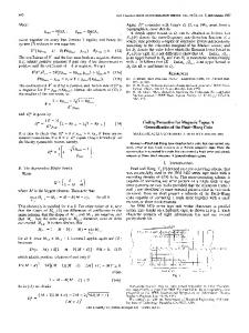
such that {Ξ(x, x0 ) ≥ 0} is the set of visible regions and {Ξ(x, x0 ) < 0} is the set of invisible regions from x0 . Enumerate all the points yi ∈ P . Define a projection operator πx0 : Rd → S d−1 , mapping a point onto a unit sphere centered at x0 . Then define a piecewise constant approximation to ρx0 by ρ˜x0 (z) := min{ρx0 (z), |x0 −yi |}, for every yi ∈ πx0 B(yi , ǫ), (3) where ǫ > 0 is chosen as in [1]. Analytically, ρ is piecewise continuous with jumps corresponding to the location of horizons, i.e. points where ν(x, x0 ) · n(x) = 0, n(x) is outer normal vector to the occluder’s boundary. Smoothness of ρ in each its continuous piece corresponds to smoothness of visible portion of the occluding surface. We use discontinuity preserving Essentially Non-oscillatory (ENO) interpolation introduced by Harten et al. [2] to construct a piecewise p-th order EN O(p) polynomial approximation ρx0 to ρx0 from ρ˜x0 . Our EN O(p) approximation ρx0 is then used to compute derivatives on the occluding surfaces (away from the edges) and easily extract various geometric quantities, such as curvature. Fig. 1 depicts visibility map obtained via (2) and Fig. 2 illustrates corresponding ρEN O(4) , its derivatives, and curvature.
III. V ISIBILITY I NTERPOLATION The visibility formulation from [1] is described below. It is then applied to the problem of environment exploration by single and multiple observers. The range-sensor attached to an autonomous vehicle is used to sample data from opaque objects in the environment. The obtained point cloud is then sampled onto a sphere centered at the observing location and interpolated to accurately represent visible boundaries of occluding objects. The following construction of visibility was introduced in [1]. Assume a point cloud P is uniformly sampled from the occluding surfaces in the bounded domain Ω by the range sensing device. Given a vantage point x0 and a point x in Ω, let ν(x0 , x) := (x − x0 )/|x − x0 | be the view direction from x0 to x. For any direction defined by a unit vector p construct a piecewise continuous function on a unit sphere: ½ minx∈Ω {|x − x0 | : ν (x0 , x) = p}, if exists ρx0 (p) := ∞, otherwise (1)
Fig. 1. Visibility map generated from artificial data: dark regions - invisible, light regions - visible, red star - vantage point (−0.2, 0.4), magenta circles - visible boundary, yellow circles - horizon points.
IV. A PPLICATION OF V ISIBILITY I NTERPOLATION TO NAVIGATION P ROBLEM In this paper we consider application of Visibility Interpolation to the problem of exploration of an unknown bounded two-dimensional region which may contain obstacles. Similarly to [16], we navigate in the environment by approaching one of the edges corresponding to horizons of the visibility function ρ defined on a unit circle. The shape of obstacles may be arbitrary. During exploration we construct a map of “seen” environment, i.e. boundaries of obstacles. We set the following restrictions on the path traveled by the observer: the path should be continuous and consist of
5426
FrB15.6 infinity
ρENO(4)
1
0
−3
−2
−1
0 1 θ (radians)
2
3
−2
−1
0 1 θ (radians)
2
3
−2
−1
0 1 θ (radians)
2
3
−2
−1
0 1 θ (radians)
2
3
dρENO(4) / dθ
1 0 −1 −2 −3 −4 −3
d2ρENO(4) / dθ2
10 8 6 4 2 0
Curvature of ρENO(4), κ
−3
0 −5 −10 −15 −20 −3
Fig. 2. ENO interpolated visibility function ρENO(4) (θ) corresponding to Fig. 1 with edges marked by red circles; first and second derivatives of ρENO(4) (θ), and the curvature.
discrete steps; the number of steps should be finite, and the total distance traveled must be finite. Below we first introduce the basic algorithm for a single observer. Then we describe its extension to multiple observers. Algorithm 1 (Single observer). 1) For the given x0 outside the occluding objects construct the visibility function ρx0 (θ); 2) Find all the discontinuities (edges) on the (θ, ρx0 (θ)) map and choose the edge to approach, say, in the direction of θe (store unexplored edges in a list). The choice of an edge depends on particular aspects of the problem and will be discussed below. If ρx0 (θe ) < ρx0 (θe + δ), choose the direction θe + δ; Else choose the direction θe − δ; here δ is chosen so that the observer does not approach the obstacle closer then some fixed distance parameter λ. 3) Move x0 ¡along ¢ the chosen direction by amount r = min{tan π3 κ1 , d}, where κ is the curvature of an edge and d is a parameter controlling the maximum stepsize. If κ = 0, shift x0 by small amount to see the next edge.
4) Finish when all the edges are “removed” from the list; otherwise proceed to Step 1 with current location of x0 . The above algorithm always converges. Its optimality depends on the choice of edge in Step 2. In [1], the nearest edge to the observer at x0 is chosen, as opposed to the random edge in [16]. Another alternative would be to approach the edge with corresponding largest curvature κ, which maximizes the area revealed. In our experiments, the choice of the next edge to approach in Step 2 is dictated by the specifics of the sensor design described in section V. We prefer to move around the obstacles in the counter-clockwise fashion to minimize the effects of errors produced by the sensors. Thus, in Step 2 of Algorithm 1 we choose the right-most edge of the object. Consider the following extension for multiple observers. Let {xj }nj=1 be a set of observing locations. Also, let Ξj be a visibility indicator map defined by (2) corresponding to xj . In addition, let Θj = {θj,1 , . . . , θj,k } be a set of edges visible from the vantage point at xj . The algorithm for multiple observers is as follows. Algorithm 2 (Multiple observers). 1) For each xj outside the occluding objects construct the visibility function ρxj (θ); 2) Compute Ξ = maxj {Ξj }; 3) Find the set of edges Θj corresponding to each xj . For each j, exclude those θj,k for which Ξ ≥ 0; 4) If there remain edges for observer at xj to approach, do so as in Algorithm 1, Steps 2 and 3; Else move observer at xj in the direction perpendicular to the direction of the nearest xi to see new edges; 5) Finish when all the edges are “explored”; otherwise go to Step 1 with current locations xj . Note that in Step 3 of the above algorithm we are excluding those edges corresponding to xj , which are visible by another observer xi and thus do not need to be further explored. The perpendicular move in Step 4 is chosen to maximize chance of “seeing” more new area. We would like to remark on different modes of execution of Algorithm 2. In concurrent mode all observers process sensor data simultaneously. This way, the next vantage point of each observer depends only on their previous positions. In sequential mode the observers are ordered as a sequence, and only one may move at a time. In this situation, position of the next observer depends on new positions of previous observers. The ordering may change according to decision to optimize joint visibility. Further details on these algorithms will be reported in a forthcoming paper [20]. In our experiments, we implement the concurrent mode. Results of implementation of Algorithm 2 will be discussed in detail in section VI. V. T EST- BED AND R ANGE S ENSORS The results in this paper were obtained using the second generation [3] of an economical micro car test-bed developed
5427
FrB15.6 The sensor must be mounted so that the line between LED output and receiver is parallel to the ground (see Fig. 3) to minimize the effect of sensor sensitivities to the boundaries, i.e. sharp differences in texture or color of the object. For simplicity, we have idealized our environment by covering the occluding objects with white paper for uniformity in color, texture, and reflected ambient light. Here we describe the process of sensor data calibration. The sensor takes readings at a rate 25 Hz. Sensor readings are produced by Analog Digital Converter (ADC), which outputs values proportional to voltage output (V×204.8). The raw data obtained from the sensor over a period of several seconds is depicted in Fig. 5. We use the most frequent reading as the value at current position. In Fig. 6 we plot values at given distances from the object measured along the normal to the surface of an object. 290 ADC output (V×204.8)
in [21]. The purpose of the test-bed is to design a cost effective platform to study cooperative control strategies. The dimensions of the test-bed floor are 200×160 cm. The second generation vehicles communicate at 30 Hz and possess onboard processing and onboard range sensing. Tank-based vehicles with caterpillar-style drive are used to allow for a zero turning radius. The tank has dimensions 7 × 3.8 × 4.6 cm and weighs 65 g with batteries. Such a tank is depicted in Fig. 3. The position of the vehicles is tracked by overhead cameras. An off-board computer is used for communication with the overhead cameras and for processing sensor data from the vehicles. All the basic motion maneuver, sensor acquisition, and communication routine is processed onboard by a 16 MHz Atmel (Atmega 8) microprocessor. The tank drives two belts independently, resulting in turns of arbitrary radius, while moving forward and backward. One can obtain more details about the test-bed and the vehicles in [3].
270
250
230
210 50
100
150 Sample number
200
250
300
Fig. 5. Sensor ADC output 60 cm away from the object; green line corresponds to the most frequent value.
Fig. 3.
Tank with the attached sensor.
Now we shall describe the range sensors used in our experiments. We work with sensors manufactured by Sharp (model 2YOAO2 F58) of range 20 − 150 cm. The sensors are equipped with a PSD onto which the light is focused. IR EM radiation is emitted via LED at the front of the sensor. The wavelength range in use is 850 nm ± 70 nm. The halfintensity angle of the device is 1.5◦ . See Fig. 4 for schematic sensor layout.
Fig. 4.
Schematic sensor layout and ray patterns.
ADC output (V×204.8)
500 400 300 200 100 20
40
60 80 100 120 Distance to reflective object (cm)
140
160
Fig. 6. Sensor ADC output corresponding to distance to reflective object measured along the normal to the surface; green vertical lines mark working sensor range.
In Fig. 7 we show several range curves constructed from different angles to the surface of the object. As one can see from Fig. 7, the range calibration curves are shifted with respect to one another for different viewing angles (upward, when the object is viewed from the right, downward, when object is viewed from the left). This results in the same sensor output value for two different sensor positions. For example, sensor output at a distance of 90 cm from the object at an angle −85◦ to the normal to the surface is the same as the sensor output at a distance of 45 cm at an angle +75◦ and yet the same as the output at a distance of 60 cm along the normal to the surface. If we take as a reference the range curve measured along the normal to the surface of reflective object, we obtain
5428
FrB15.6
ADC output (V×204.8)
600 85 +75 0
500 400 300 200 100 0 0
20
40
60 80 100 120 140 Distance to reflective object (cm)
160
180
Fig. 7. Sensor ADC output corresponding to distance to reflective object measured along different angles to the normal to the surface; red marks correspond to points on the range curves with similar sensor output.
inaccuracies when looking at an object from a different angle. For example, one can see from Fig. 8 the tilt in the measured surface position with respect to the actual one. The results may be improved by taking several measurements along a given direction. This way we can find a matching range curve from which we can deduce the distance to the object and the incident angle. However, this solution is too expensive and thus we did not implement it. In addition, we note that the shift is only significant when looking at an object from the right. Thus, a path-planning algorithm is modified with a bias towards moving in a counter-clockwise manner. See Fig. 8 for an example.
after each step. The red lines mark the path of each vehicle up until its current location. Dark regions are invisible at current step and lighter regions are visible. Magenta circles represent shadow boundary obtained via ENO high order interpolation of the obtained range data. Black circles represent horizon points which will be approached in the next step. The complete visibility map is depicted in Fig. 9. It is constructed by taking the union of visibility maps of all observers at all steps. From this map, one can estimate the quantity, size, and locations of the obstacles. However, the boundaries are not accurately represented due to low sensor accuracy and small number of samples. As was mentioned above, the results may be improved by correcting for the angle of incidence of the IR beam. Overall, the quality of the results is satisfactory taking into account hardware limitations.
VI. R ESULTS AND C ONCLUSION In summary, we implement a multi-vehicle environment mapping algorithm based on a Visibility Interpolation formulation introduced in [1]. The algorithm does not require any shape priors for the occluding objects. We use two boxes as our sample obstacles for easy representation. The positions, shapes, and quantities of obstacles are unknowns. Two tank-based vehicles equipped with the range sensors are initially positioned on the test-bed floor outside the obstacles. Each tank makes a 360◦ sweep to gather range data from its surrounding environment. About 80 samples are taken in one sweep. Each sweep takes less then a minute to complete. Then, a visibility map and next position of each vehicle is computed off-board based on sensor output. The next observer’s position is transmitted to the robots and they proceed to collect data from new vantage point. This process is repeated until the whole region has been explored as in Algorithm 2 above. In the example, exploration took two steps by each observer. The obtained range data is fit to the range calibration curve in Fig. 6 via cubic interpolation. Then the data is processed in the following way. Whenever we get a hit which is outside of the range of the sensor or its x, y position is outside the test-bed floor, we assign the value of “infinity”, which is set to be at 120 cm. Joint visibility maps after each step are depicted in Fig. 8. Actual obstacle boundaries are represented by yellow lines on each figure. Red stars represent positions of the robots
Fig. 8. Exploration of environment with 2 observers. Red stars are observers’ positions; magenta circles are the sensor output converted to range data; big dark circles are the next edges to be approached; yellow boxes are the actual obstacle outlines; dark regions are currently invisible; light regions are currently visible.
5429
FrB15.6 160 140 120
y (cm)
100 80 60 40 20 0 0
20
40
60
80
100 120 x (cm)
140
160
180
200
Fig. 9. Map resulting from the environment exploration. Dark regions are invisible and light regions are visible. Yellow boxes are the actual outlines of obstacles.
VII. ACKNOWLEDGEMENTS This research was supported as part of the Research in Industrial Projects for Students (RIPS) program at the Institute for Pure and Applied Mathematics (IPAM), and funded by NSF grant DMS-0439872 and NSA grant H9823006-1-0057. We would like to thank Matthew Sottile who was a RIPS industrial mentor from Los Alamos National Laboratory. Additionally, this research was supported by NSF grant DMS-0601395, ARO MURI grant 50363-MAMUR, ONR grant N000140610059, ARO grant W911NF05-1-0112, and NSF grant DMS-0513394. R EFERENCES [1] Y. Landa, R. Tsai, and L.-T. Cheng, “Visibility of point clouds and mapping of unknown environments”, Advanced Concepts for Intelligent Vision Systems, ACIVS 2006, Sept 18-21, 2006, University of Antwerp, Belgium (preprint available as UCLA CAM report 06-16). [2] A. Harten, B. Engquist, S. Osher, S.R. Chakravarthy, “Uniformly high order accurate essentially nonoscillatory schemes, III,” Journal of Computational Physics, 71, (1987), 231-303. [3] K. K. Leung, C. H. Hsieh, Y. R. Huang, A. Joshi, V. Voroninski, and A. L. Bertozzi, “A second generation microvehicle testbed for cooperative control and sensing strategies”, submitted to ACC (2007). [4] W.-P. Chin and S. Ntafos, “Shortest watchman routes in simple polygons”, Discrete Comput. Geom., 6 (1991), 9-31.
[5] J. E. Goodman, J. O’Rourke, editors “Handbook of discrete and computational geometry”, CRC Press LLC, Boca Raton, FL; Second Edition, April (2004). [6] J. Urrutia. “Art gallery and illumination problems”, in J. R. Sack and J. Urrutia, editors, “Handbook of Computational Geometry”, 973-1027, (2000). [7] Y.-H. R. Tsai, L.-T. Cheng, S. Osher, P. Burchard, G. Sapiro, “Visibility and its dynamics in a PDE based implicit framework” Journal of Computational Physics, 199, 260-290, (2004). [8] S. Osher, J. A. Sethian, “Fronts propagating with curvature-dependent speed: algorithms based on HamiltonJacobi formulations”, Journal of Computational Physics 79 (1) 12-49, (1988). [9] L.-T. Cheng and R. Tsai, “Visibility optimizations using variational approaches”, Communications of Mathematical Sciences, 3, (3) (2005). [10] F. Wolf, A. Howard, and G. S. Sukhatme. “Towards geometric 3D mapping of outdoor environments using mobile robots”, IEEE/RSJ International Conference on Intelligent Robots and Systems (IROS),1258-1263, (2005). [11] D. Murray and C. Jennings. “Stereo vision based mapping for a mobile robot”, Proc. IEEE Conf. on Robotics and Automation, (1997). [12] B. Tovar, L. Guilamo, and S.M. LaValle, “Gap navigation trees: minimal representation for visibility-based tasks”, Proc. Workshop on the Algorithmic Foundations of Robotics, (2004). [13] B. Tovar, S. M. LaValle, and R. Murrieta, “Optimal navigation and object finding without geometric maps or localization”, Proc. IEEE International Conference on Intelligent Robots and Systems, (2003). [14] B. Tovar, S. M. LaValle, and R. Murrieta, “Locally-optimal navigation in multiply-connected environments without geometric maps”, IEEE/RSJ International Conference on Intelligent Robots and Systems, (2003). [15] B. Tovar, S. M. LaValle, and R. Murrieta, “Optimal navigation and object finding without geometric maps or localization”, IEEE International Conference on Robotics and Automation, (2003). [16] B. Tovar, R. Murrieta-Cid, and S. M. LaValle “Distance-optimal navigation in an unknown environment without sensing distances”, IEEE Transactions on Robotics, (2006). Under review. [17] F. Zhang, A. O’Connor, D. Luebke, and P. S. Krishnaprasad, “Experimental study of curvature-based control laws for obstacle avoidance”, Proceedings of the 2004 IEEE International Conference on Robotics and Automation, New Orleans, LA, April (2004). [18] F. Zhang, E. Justh, and P. S. Krishnaprasad, “Steering control, curvature and Lyapunov navigation”, preprint, (2003). [19] A. Ganguli, J. Cortes, F. Bullo, “Distributed deployment of asynchronous guards in art galleries”, Proceedings of the 2006 American Control Conference, Minneapolis, MN, June 14-16, (2006). [20] Y. Landa, R. Tsai, “Mapping unknown environments from range data using multiple observers”, (2006). [21] C. H. Hsieh, Y.-L. Chuang, Y. Huang, K. K. Leung, A. L. Bertozzi, and E. Frazzoli, “An economical micro-car testbed for validation of cooperative control strategies”, Proceedings of the 2006 American Control Conference, Minneapolis, MN, June 14-16, 1446-1451, (2006).
5430