Robotized Task Time Scheduling and Optimization Based on Genetic Algorithms for non Redundant Industrial Manipulators Khelifa Baizid, Amal Meddahi,
Ryad Chellali, Hamza Khan,
DIEI, University of Cassino and Southern Lazio, Cassino, Italy (
[email protected]) Ali Yousnadj EMP, Polytechnics Military School, Algiers, Algeria, (
[email protected])
PAVIS, ADVR, Istituto Italiano di Technologia Genova, Italy, (
[email protected],
[email protected]) Jamshed Iqbal, COMSATS Institute of Information Technology Pakistan, (
[email protected])
Abstract—Industrial robot manipulators must work as fast as possible in order to increase the productivity. This goal could be achieved by increasing robots speed or/and optimizing the trajectories followed by robots while performing assembly, welding or similar tasks. In our contribution, we focus on the second aspect and we target the shortening of paths between task-points. In other words, the goal is to find the shorter traveled distance between different configurations in the coordinate space. In addition to the short distance goal, we aim as well to impose both IKM (Inverse Kinematic Model) and the relative position and orientation of the manipulator regarding the task-points. To this end, we propose an optimization method based on Genetics Algorithms. The method is validated via numerical and graphical simulation, where, results show that the total cycle time required to perform a spot-welding task of an industrial car-body by a 6-DOFs (Degree Of Freedoms) industrial manipulator was drastically reduced. Keywords—Industrial optimization
I.
manipulator,
genetic
algorithms,
INTRODUCTION (HEADING 1)
Nowadays, robot manipulators integrated into manufacturing systems must work as fast as possible in order to increase the productivity and decrease the production costs. The need of proper methods to define robotized tasks leads to develop various tools and methods to improve the quality of the final product. Moreover, several features such as manipulators flexibility, versatility and adaptability help to achieve many tasks within large environment variations [1][2]. Taking into consideration the complexity of the manipulators kinematics and the manufacturing system, a better exploitation may be achieved by involving optimization techniques and offline programming procedures [2]-[4], that drives the end product to have high quality and low cost. Usually, researches on robot manipulators trajectory optimization focus on repetitive tasks such as spot-welding, laser and water cutting handling parts, and many other applications [5]-[9], where the order of the task points’ does not affect the achievement of the task. However, to visit all these points, the total cycle time can be affected by the order of achievement, especially when the robot manipulator must return to its initial configuration. Namely, the task points order
978-1-4799-4926-7/14/$31.00 ©2014 IEEE
has an important effect on the cycle time execution; because the minimum cycle time is related to the minimum traveled displacement of the manipulator joints. Indeed, this problem is very similar to the Traveling Salesman Problem (TSP) [10], where a salesman has to visit a defined number of cities starting and ending by the same location. TSP’s objective is to find the minimum traveling tour varying the inter cities distances to reach all cities. For robotics tasks, the problem is more complex. Indeed, the traveling tour has to be performed in coordinate space rather than operational space with higher dimensionality (6 instead of 2 for the TSP planar case). Furthermore, many other factors can affect the task achievement and the cycle time such as the robot manipulator placement and orientation [11]. Lots of researches have inspired from TSP by implementing Genetic Algorithms (GAs) [8][12]. The weakness of these methods is the non-consideration of the multiplicity of the IKM configurations (Inverse Kinematic Model) of the manipulator: the fitness function is calculated according to the path traveled by the robot manipulator and the average speed of its joints. Authors argued that these methods have a good impact even with a large number of the taskpoints. However, only 2-DOF (Degree Of Freedoms) or 3-DOF manipulators were considered. Considering point-to-point tasks, authors in [8] generalized existing methods to cover robots with more than 3 DOF. In addition, they included the order of the task-points and the multiplicity of the IKM configurations. Moreover, they added obstacle avoidance aspects in [13]. Another method using TSP considering continues trajectories were addressed in [14]. Nevertheless, for most of these methods, the robot manipulator placement and orientation was missing. In [15], authors tackled the problem of the task-point order and the multiplicity of IKM configurations by considering also the manipulator placement and achieved important results in line with the findings in [16][11] about that the influence of robot manipulator placement and orientation on the total cycle time. In this work we propose a method based on GAs that takes advantage of both CAD SolidWorks system to simulate and optimize the cycle time and the effectiveness of GAs based methods in solving TSP-like optimization problems [8][13][14]. Our method is dedicated to non-redundant
industrial robot manipulators and considers all the parameters mentioned previously. Thus, the developed algorithm handles a more challenging optimization problem in a high dimension space including four parts: 1) the chain of N task-points that the end-effector of the robot manipulator has to visit, 2) the robot’s IKM configurations, 3) the relative placement between the manipulator and the task-points, 4) the relative orientation between the manipulator and the task-points. Furthermore, we provide the statistics of the cross effects of parts (one by one, two by two, three by three and the last that combines all parameters together). This analysis allows showing the importance and the influence of each part on the algorithm's performances. It is worth to noting that the issues of obstacle avoidance in out method is resolved by intermediate points. The paper is organized as follows: the problem statement is given in the second section; the third section describes the proposed optimization approach; the fourth and the fifth sections present the simulation setup and discuss the obtained results respectively; the sixth section gives our conclusions. II.
point of the task with m different IKM configurations, and it can be located into a certain position and orientation zones (a set of positions and orientations). Consequently, the purpose is to find the tour (traveled distance) to visit all task-points that correspond to the smallest time; considering the multiplicity sequences of the task-points order, IKM configurations, the manipulator placement and the orientation. At a given position and orientation of the manipulator ( x, y, z , , , ) ( used to calculate the transformation from the task-points frame FT to the manipulator fixed frame FM ) the time ti needed by the manipulator to travel from the point i 1using the k th IKM configuration to the point i using the l th IKM configuration is defined by the equation (2): ti
ql max
ji
qk
j ( i 1)
qj
j 1,2,..., n
(2)
PROBLEM STATEMENT
In robotized manufacturing plants, the time required to perform a given task (cycle time) depends on the traveled distance by the manipulator, which is related to the sequence of the task-points visited by the end-effector (task-points order). On the other hand, the manipulator executes the task in the operational space and performs the motion in the coordinate space, which makes the traveled distance depending from the manipulator’s IKM. Thus, the optimization problem is concerned with finding the minimum distance between each two consecutive ordered task-points. Moreover, the IKM is strongly affected by the placement and the orientation of the manipulator. Hence, the cycle time needed by the manipulator to perform a given task is a function of the order of achievement of the task-points, the IKM at each task-point, the manipulator placement and orientation. Some previous works considered, only, the order of visiting and the multiplicity of the IKM such as in [8], while, in [15] authors considered the manipulator placement, in addition. In this work, our objective function incorporates the orientation of the manipulator, in addition to these tree parameters. Similarly to [15] and [8] we compute the cycle time based on the displacement of the manipulator joints between each consecutive pair of points and the average velocity of the corresponding joint. Let us consider a 6-DOFs manipulator (Fig.1); that has to visit N points, which represent the required task in 6 dimensional space (3 positions and 3 orientations) and return back to its initial configuration. The relation between the coordinate space and the operational space is given bellow: (1) P(t) f q(t) Where q (t ) R n is the vector of joint coordinates in the coordinate space, n is the number of DOFs of the manipulator, P(t ) R N is the path to be performed in the operational space, and f denotes the IKM of the manipulator [17]. It is worth to mention that the solution of the IKM at a given task-point i exists if P , where represents the workspace of the manipulator. The manipulator can reach each
Fig. 1.
A schema of a manipulator with n-DOFs and visit N points
Where, k 1,2,..., m is the IKM configuration used at the task-point i and l 1,2,..., m is the IKM configuration at the task-point i 1. Consequently, q kji is the displacement of the joint j at the task-point i , that is associated to the position and the orientation of the manipulator . Whereas q is the
j th
j
manipulator average joint's velocity. It is worth mentioning that the maximum used in equation (2) is over the time spent by njoints to travel between the points i-1 and i. The total cycle time of a given task tc is defined by the equation (3): t c
N 1
t i 1
i
(3)
Where N 1 represents the number of distances traveled between each two successive configurations plus the return to the initial configuration. To this end, the overall formulation function of the optimized task's time can be written as follows: N 1 . top min ti j, i, k , l, q j , N , ( x, y, z, , , ) i1
(4)
In order to find the minimum cycle time, we must probe all the possible solutions given by (4), which is an intractable issue compared to the problem tackled in [8] and [17]. For instance, the number of IKM configurations of a manipulator of 6 DOFs is 28 [18]; and this number can be reduced to 24 in the case the manipulator has the last three axes intersected. Therefore, the number of the possible IKM configurations at each point of the task can be expressed as 2d where d 1,2,3,4 ; and (2d)N for the total task-points number. Additionally, the possible number of the task-points order is defined by N!, this number can be reduced to the half because of the symmetry (e.g., the visiting order of a given points 1-2-3 in this sequence is the same as 3-2-1). While, the
number of placements and orientations of the manipulator, with respect to the task-points, is related to the number of grids that construct the placement and orientation zones , which are calculated using the 3D models of the task-points and the manipulator as described in [11]. Let us define 1 and 2 positive numbers related to the placement and the orientation zone respectively. The possible placement number is: (5) 1 xnode ynode znode where xnode, ynode and znode are the integer placements' number on x, y and z axes respectively. Similarly, the number of orientation is: 2 node node node (6) The whole number of possible solutions is related to all cited parameters, including the placement (5) and the orientations (6), which can be summarized as: N sol
1 * 2 * N! * 2d 2
N
Fig. 2.
Chromosome of n-DOF manipulator visiting N points in 3D space.
(7)
The search space is significantly high. Taking an example of 6-DOFs manipulator that has to perform 10 points with d=3 and ɛ1= 10e3, time to probe all solutions is 2.8002e+09min. III.
Fig. 2 shows the chromosome form of the problem tackled in section 2. As shown, the manipulator performs the task starting by visiting the point number 22 using the configuration coded by the binary digits “10…1” , then visits the point 3 using the configuration coded by the binary digits “01...0” and it finishes by visiting the point number 6 using the configuration coded by the binary digits “11…1”; the relative placement of the manipulator and the task-points is on the nodes of “01...0”, ”10...0” and “00...1” corresponding to the three coordinate axis x, y, z respectively; relative orientation of the manipulator and placement are situated on nodes “01...1”, “10...0” and “01...1” around x, y, z axes respectively.
GAS OPTIMIZATION APPROACH
Genetic algorithms are stochastic optimization methods introduced by John Holland based on the Darwinian evolution theory [19]. A genetic algorithm is a sort of artificial evolution of a population of chromosomes, which represent the possible solutions to the concrete problem. First, the initial population is generated randomly, and then it is evolved through several operations within a number of generations. At every generation, the fitness (objective function) of each chromosome is evaluated with respect to specific conditions, and then the best chromosomes are selected in order to be reproduced within the next generation. The reproduction procedure generates new offspring based on the genetic material of two parent chromosomes, by applying the crossover and mutation operations with a certain selection probability. Each chromosome is composed of four parts: the visiting order of the task-points (first part), the manipulator IKM configurations in each point (second part), the manipulator relative placements (third part) and the manipulator relative orientations (fourth part). The best solution is selected based on the fitness function, which is calculated based on (4). A. Coding Process The first issue of any method based on genetic algorithm is the proposition of an adequate representation to encode the objective function of the optimization problem. This encoding can be implemented either by natural or by binary alphabets on which originally the theoretical foundation of GAs are implemented. In our case, the first part of the chromosome must be encoded by integer values, since the random selection process (in the crossover and mutation operations) may provide the same alphabet, which creates serious conflict phenomena in the case of binary encoding. Consequently, we developed a specific algorithm to correct bits that lead to the same genes; in order to avoid the redundancy of the visited point part. For the second, third and forth parts we implemente binary encoding.
B. Optimization Process In our approach, a population of 50 chromosomes is generated randomly and reproduced over 3250 generation. The evaluation process is applied according to the objective function described earlier, which is based on the cycle time that each solution can produce; where solutions with minimum time (high fitness value) are selected for reproduction. The selection constraint is a rank based selection where an elitist fraction of 10% is preserved unchanged (no mutation or crossover) from the current generation to the next, to guarantee that the best solutions will not be lost. The remaining population’s chromosomes are reproduced through a mutation and crossover probability of 0.1 and 0.98 respectively. The applied crossover is the uniform crossover because it performs well compared to the two-point crossover, because this last leads to generate non-homogeneous chromosomes in our optimization. IV.
SIMULATION SETUP
A. 3D modeling and task definition of the robotized site To evaluate the proposed approach we have selected a real world industrial example of an automation plant with a 6DOFs industrial manipulator (Staubli RX-130 XL). The task of spot-welding has been chosen because of its obvious importance for many industrial plants, especially in cars body assembly field. To this end, it is necessary to develop the whole 3D model of the robotized site, including the manipulator and its workspace, the working environment, the desired task-points and the pieces to be assembled (Fig. 3). The coordinates of the task-points are distributed on the whole body of the car. The definition of these points is done by using CAD-learning technique illustrated in [20]. The size of the occupied task zone is: 1695.75mm, 286.18mm and 479.98mm on x, y and z axes respectively. After the definition of the 3D model of the task, we calculate the placement and the orientation zone as discussed in [11]. Their values are respectively: 290.46[mm], 290.50[mm], 302.12[mm], 119.89°, 223.94° and 246.59 for x, y, z, α, β, δ respectively.
B. Case of study To examine the effectiveness of the proposed approach, we evaluate the time of the task in five stages to quantify the influence of each part in the optimization process, separately and with different possible combinations (one by one, two by two, three by three and all parameters together) (Table 1). The simulations are for objective to optimize the cycle time of the task needed by the manipulator to perform the spot-welding at all task points and return back to the initial configuration. To seek precise results, the optimization process of each combination is performed within 10 trials.
not due to a local minima because the nature of the algorithm does not allow these issues to happen [19]. This indicates that this part is dominating in the optimization process. However, the variance value of the other parts (respectively: 3.88s, 31.97s and 15.23s) illustrates their ability to improve the solution. It is very worth to notify that the given time by each part is, strongly, related to the fixed values of the other parts.
Fig. 4.
Fig. 3.
3D model of the robotized site.
TABLE I. POSSIBLE COMBINATIONS OF THE CHROMOSOME (T: TASK POINTS ORDER, C: IKM CONFIGURATIONS, P: PLACEMENT, O: ORIENTATION). 1st stage 2nd stage 3rd stage 4th stage 5th stage
T T-C T-C-P
V.
C T-P T-C-O
P O T-O C-P T-P-O C-P-O T-C-P-O Overview of all stages
C-O
P-O
RESULTS AND DISCUSSION
In this section we assess the proposed optimization approach by calculating the time of the task according to the plan detailed in the previous section. For the GAs operators such crossover and mutation rates are chosen 0.9% and 0.05%, respectively. In order to have precise analyses, we used ANOVA (analyze of the variance) technique for our comparison at all stages except at the fourth and the fifth ones. Since the GAs are stochastic algorithms we use term of "near optimal" instead of term "lower bound" of the task's time, which indicates the best time found by the algorithm. First stage: As mentioned in Table 1the, this evaluation test consists of the optimization the cycle time according to each part separately (see), starting from a random population. Fig. 4 shows the mean of cycle time that each part reaches. In details the T part reaches the value of 39.17s, while the C part reaches better value of 29.01s (best time in this scope). P and O parts got very closer with times of 46.54s and 47.95s, respectively. The p-value or the significance of the difference is very small (3.07e-011) which indicates a considerable difference among these parts. Moreover, this can be observed, simply, from the cycle time difference among these combinations, which attains the maximum value of 18.94s. The variance of the C part looks smaller because during most of trials, the optimization process has reached a close value sets (best possible solution for a given combination), where the best solution can't be improved further. It is worth noting that this is
Comparison among parts separately.
Second stage: In this stage we present the time of the task based3.0729e-011---39.17--------29.01------------46.54--------------47.95 on the combination of different parts two by two, where var: 34.756=.......== 3.8851==.......==31.9733==......==15.2394= the level of complexity is augmented comparing to the previous stage. Considering the first combination that includes T and C, we set the P and O parts (which are generated randomly at the first generation) to fixed values. Successively, we combine the T with the P and then with the O, where we fix the C and the P parts, respectively. We do the same with the C, P and O parts, later (Fig.5 shows all combinations). The p-value (i.e., the significance of the test) of 8.31e-025 clearly shows the meaning of the difference between these combinations. The first observation is that the combinations of the T part with the C part and this last with the P give best solutions. Values of the best cycle time that have been found are respectively 24.96s and 25.85s. This indicates that the T-C performs better, however, C-P's variance ( 7.87sec) is bigger compared to the ones of T-C, which indicates the diversity of the found solutions. Some of these solutions reach values less than the one given by T-C, which indicates the possibility of finding solutions better compared to the combination of T-C. The variance of T-C is smaller which indicates that this combination always converges to near optimal solutions. However, when we consider the one outlier of 22.79s (which is less than T-C's mean value) seems there are some exceptions that can appear due to the chosen values of P and O parts. Moreover, the C part seems to be more dominating by giving the third best time of 26.75s in this series, combined with the O part. The T part combined with the P part gives better results with comparison to the same part combined with O. Respectively values of the found mean cycle times are 34.91s and 37.82s. However, with regarding to the possibility of finding best solutions, seems that the T-O performs better by having an interval of solutions varies from 31.36s to 39.82s (with variance of 7.08s) over the 10 trials. This may tell us about the complexity of convergence (does not converge to the best possible solution at all trials) and the huge space of solutions, which is increased by the fact of considering the O. Comparing this to T-P, the found solutions are very diverse from each other, and this may allows the algorithm to find best solutions by playing on the GAs parameters [15].
Finally the combination of the part T and the part O seems to give less performances, this is due to the reduced space of solutions affected by the fixation of the T and the C parts. However, by considering the variance value of 14.73s (the largest in this scope), the algorithm can reach best cycle time than the given mean value. Generally, P and O increase the performances of the T and C during the optimization process. For instance, with respect to the First stage, the part T reduces the cycle time from 39.17s to 34.91s and 37.82s, combined with P and O parts, respectively. Similarly for the C part, it improves the cycle time from 29.01s to 25.85s and 26.75s when it is combined with P and O parts, respectively. These improvements are without considering essential parts such as the part T for C-P and C-O, and the part C for the combinations of T-P and T-O.
Fig. 5.
Fourth stage: In the fourth stage we combine all parts together in order to benefit from all of them at ones. to find a best near optimum cycle time. The chromosome size becomes even longer. Effectively, this increases the chance of finding best results; however, it may takes more computational time in term of generations (after how many generations the algorithm converge). Unlike previous stages, without using ANOVA technique, we present in Fig. 7 the worst and the best cycle time at each generation, at one of the best trials. By launching all parts at the same time, we get impressive results, where the 10 trials mean of the cycle time reaches 17.61s, while the worst time value is 82.92s. These is appreciated results with comparing to previous combinations (separately, two by two and three by three).
Task time evaluation by combining parts two by two.
Third stage: In this stage, we combine different parts three by three. In this stage we increase the level of complexity (related to the search space) by considering more parts. The chromosome size becomes much longer. In this stage the optimization process performs well for finding the best solution compared with the previous stages as it is shown in Fig. 6. The best mean value of the cycle time is given by the combination of T with C and P parts, where, the cycle time is reduced to 21.93s. While, the second best time, in this stage, is given by the combination of T with C and O by reaching the value of 25.45s; the third best time found in this scope is 25.75s, from the combination of C with P and O parts. While the worst time is given by the combination of T with P and O parts by value of 31.68s.
Fig. 6.
Especially, by playing on the number of the generation, which is limited in our case due to some constraints of VBA. On the other hand, we can see how much the O part improves the results at some trials and makes it worst in others. Also, other combinations (T-P-O and C-P-O) have improved the cycle time with regarding to T-P and C-P respectively. Moreover, the variance increases to reach the value of 4.57s and 6.72s for TP-O and C-P-O, respectively, which also may indicate the possibility of finding best solutions.
Task time evaluation by combining parts three by three.
However, the overall observation on this stage is the improvement of the performances of the algorithm compared to previous two stages. In detail, the T-C improves its solution of the cycle time from 24.96s to 21.93s. When adding the O part to T-C the mean time seems worst, however, by considering the T-C-O's variance of 4.40s, definitely, we expect that the algorithm can reach best values than T-C mean.
Fig. 7.
Maximum and minimum task's time optimization.
Also it is clear that the near optimal time that has been found is a contribution of all parts together, (i.e., separately or with less combinations the algorithm can't reach this value). The cycle time has been reduced, in this stage, from 37.64s to 17.61s with a value of 23.23s. These results seems very promising (considering the number of task-points of 22) compared to the one presented in [15] with a reduced time of 7.66s (with N=12, and without considering the orientation). Let us define a ratio of the reduced time per point, the ratio of the proposed algorithm is 1.0559[s/point] (23.23/22), while the one given in [15] is 0.6383[s/point]. Moreover, this explicitly indicates that the proposed algorithm performs very well, even considering, relatively, high number of task-points, which also increase the level of complexity to find near optimal solutions. Fifth stage: In this stage we give an overall view of all combinations, where we compute the mean of the cycle time given by each stage. This may allow us to quantify the combinations themselves and classify which one has more influence on the optimization process. Fig. 9(a) shows the mean of the best time given by each combination and the mean of the best time at each stage. Clearly, we can see that combining different parts of the optimization process brings
important advantages to this last. Consequently, each part is benefiting from the others, and all parts push the optimization process toward the optimal solution, by improving each chromosome of the population. The best cycle time (Fig. 8(a)) compared to the previous stages is very less. Contrary the computational time (represented as the minimum number of generation to find the best solution) is higher, because the search space is increased and even within a high generation number the algorithm is still finding alive solutions. The gain of reducing the time from 37 to 17 is very significant. E.g., considering an automobile plant which produce 1500 vehicles/day (about one car/minute); reducing the cycle time of the robotics chain to the half (17/37) drives to double the production to be 3000/day. This is not negligible given that an eventual cost of a second chain (infrastructures, personals, maintenance, etc.) is dramatically high. It is very worth to not that the algorithm runs around 29min to find a near optimal solution, instead thousands of years to probe all possible solutions.
time are classified as follows: the IKM configurations, the task-point order, the placement and the orientation. Moreover, the placement and the orientation enhance the quality of the solution by increasing the search space solution. Moreover, the computational time has been reduced to a set of minutes instead of thousands of years to probe all possible solutions. REFERENCES [1] [2] [3] [4] [5] [6] [7] [8] [9]
(a)
[10] [11]
[12] [13] [14] (b) Fig. 8. Comparison of all stages, by their mean of : (a) the best near optimal time, (b) the minimum number of generations to fine a best solution.
VI.
CONCLUSION
We proposed in this paper, a novel task scheduling and optimization approach based on Genetics Algorithm (GAs) dedicated for industrial manipulators. The proposed approach takes into consideration the task-points order, the IKM configuration used at each task-point, the manipulator placement, and orientation. All these factors are combined together to participate in finding the best combination that lead to the minimum cycle time. Moreover, we sought to perform a direct comparison between all these factors, using ANOVA (Analysis of variance) that quantify the quality of each factor in reducing the cycle time. Results of these comparisons show that the factors that have the most important effect on the cycle
[15]
[16]
[17] [18] [19] [20]
M. Dissanayake, J. Gal, “Workstation planning for redundant manipulators,” International Journal of Production Research, vol.32, no. 5, pp. 1105–18, 1994. K. Shin, N. Mckay, “Selection of near minimum time geometric paths for robotic manipulators,” IEEE Trans Automat Control, vol.31, no. 6, pp. 501–11, 1986. S. Dubowsky, T. Blubaugh, “Planning time-optimal robotic manipulator motions and work places for point-to-point tasks,” IEEE Conference on Decision and Control, Ft. Lauderdale, FL, 1985. Bobrow, J. E., Dubowsky, S., and Gibson, J. S. 1985. Time-optimal control of robotic manipulators along' specified paths. Int. J. Robotics Res. 4, 3 (Fall), 3-17. L. Abdel-Malek, Z. Li, “The application of inverse kinematics in the optimum sequencing of robot tasks,” International Journal of Production Research, vol. 28, no.1, pp. 75–90, 1990. Y. Edan, T. Flash, U. Peiper, I. Schmulevich, Y. Sarig, “Near minimumtime task planning for fruit-picking Robots,” IEEE Trans Robotic Autom., vol. 7, no. 1, 1991. G.S. Tewolde, W. Sheng, “Robot Path Integration in Manufacturing Processes: Genetic Algorithm Versus Ant Colony Optimization”, IEEE Tran. on Syst. Man and Cyb., vol. 38, no. 2, pp. 278-287, 2002. P. Th. Zacharia, N. A. Aspragathos, “Optimal Robot Task Scheduling based on Genetic Algorithms,” Robotics and Computer-Integrated Manufacturing journal, vol. 21, no.1, pp. 67-79, 2005. H. Chen, W. Sheng, N. Xi, M. Song, Yifan Chen, “CAD-based automated robot trajectory planning for spray painting of free-form surfaces,” Int. Jour. of Ind. Robot, vol.29, no. 5, pp. 426-433, 2002. E. Lawer, J. Lenstra, A. Rinnooy Kan, D. Shmoys, “The travelling salesman problem,” Chichester, UK: Wiley, 1985. K. Baizid, R. Chellali, A. yousnadj, A. Meddahi, B. Toufik and J. Iqbal, “Modelling of Robotized Site and Simulation of Robot’s Optimum Placement and Orientation Zone”, IASTED 21th Modelling and Simulation, 15-17, Jul., 2010, Canada. H-S. Hwang, “An improved model for vehicle routing problem with time-constraint based on genetic algorithm,” Computers & Industrial Engineering, 42(2-4), pp. 361-369, April. 2002. Paraskevi Th. Zacharia, Elias K. Xidias, and Nikos A. Aspragathos. Task scheduling and motion planning for an industrial manipulator. Robot. Comput.-Integr. Manuf. 29, 6 (December 2013), pp. 449-462. Alatartsev, S.; Mersheeva, V.; Augustine, M.; Ortmeier, F., "On optimizing a sequence of robotic tasks," International Conference on Intelligent Robots and Systems, , vol., no., pp.217,223, 3-7 Nov. 2013. Khelifa Baizid, Rryad Chellali, Ali yousnadj, Amal Meddahi and Bentaleb Toufik, “Genetic Algorithms Based Method for Time Optimization in Robotized Site”, IEEE/RSJ International Conference on Intelligent Robots and System (IROS), 18-22, Oct., 2010, Taiwan. K. Baizid, R. Chellali, T. Bentaleb, A. Yousnaj and A. Meddahi, “Virtual Reality Based Tool for Optimal Robot Placement in Robotized Site Based on CAD’s Application Programming Interface,” Proc. of Virtual Reality Int. Conf., Laval, France, April 7-9, 2010. Khalil, Wisama, and Etienne Dombre. Modeling, identification and control of robots. Butterworth-Heinemann, 2004. L. Tsai, A. Morgan, “Solving the kinematics of the most general sixand five-degree-of-freedom manipulators by continuation methods,” ASME Mechanics Conference, Boston, October 7–10, 1984. Holland, J. H. (1992). Adaptation in Natural and Artificial Systems: An Introductory Analysis with Applications to Biology, Control and Artificial Intelligence. MIT Press, Cambridge, MA, USA. A. Meddahi, K. Baizid, A. Yousnadj and J. Iqbal, “API Based Graphical Simulation of Robotized Sites,” IASTED Int. Conf. on Robotics and Applications, Cambridge, USA, pp. 485-492, 2009.