The ASSC estimator combines Random Sample ..... To estimate the gradient of this density we can take the gradient of the kernel density estimate. 1. 1. Ë. Ë( ). ( ).
Robust Adaptive-Scale Parametric Model Estimation for Computer Vision Hanzi Wang and David Suter, Senior Member, IEEE Department of Electrical and Computer Systems Engineering Monash University, Clayton Vic. 3800, Australia. {hanzi.wang ; d.suter}@eng.monash.edu.au Abstract Robust model fitting essentially requires the application of two estimators. The first is an estimator for the values of the model parameters. The second is an estimator for the scale of the noise in the (inlier) data. Indeed, we propose two novel robust techniques: the Two-Step Scale estimator (TSSE) and the Adaptive Scale Sample Consensus (ASSC) estimator. TSSE applies nonparametric density estimation and density gradient estimation techniques, to robustly estimate the scale of the inliers. The ASSC estimator combines Random Sample Consensus (RANSAC) and TSSE: using a modified objective function that depends upon both the number of inliers and the corresponding scale. ASSC is very robust to discontinuous signals and data with multiple structures, being able to tolerate more than 80% outliers. The main advantage of ASSC over RANSAC is that prior knowledge about the scale of inliers is not needed. ASSC can simultaneously estimate the parameters of a model and the scale of the inliers belonging to that model. Experiments on synthetic data show that ASSC has better robustness to heavily corrupted data than Least Median Squares (LMedS), Residual Consensus (RESC), and Adaptive Least K’th order Squares (ALKS). We also apply ASSC to two fundamental computer vision tasks: range image segmentation and robust fundamental matrix estimation. Experiments show very promising results. Index Terms: Robust model fitting, random sample consensus, Least-median-of-squares, residual consensus, adaptive least k’th order squares, kernel density estimation, mean shift, range image segmentation, fundamental matrix estimation. 1
1. Introduction Robust parametric model estimation techniques have been used with increasing frequency in many computer vision tasks such as optical flow calculation [1, 22, 38], range image segmentation [15, 19, 20, 36, 39], estimating the fundamental matrix [33, 34, 40], and tracking [3]. A robust estimation technique is a method that can estimate the parameters of a model from inliers and resist the influence of outliers. Roughly, outliers can be classified into two classes: gross outliers and pseudo outliers [30]. Pseudo outliers contain structural information, i.e., pseudo outliers can be outliers to one structure of interest but inliers to another structure. Ideally, a robust estimation technique should be able to tolerate both types of outliers. Multiple structures occur in most computer vision problems. Estimating information from data with multiple structures remains a challenging task despite the search for highly robust estimators in recent decades [4, 6, 20, 29, 36, 39]. The breakdown point of an estimator may be roughly defined as the smallest percentage of outlier contamination that can cause the estimator to produce arbitrarily large values ([25], pp.9.). Although the least squares (LS) method can achieve optimal results under Gaussian distributed noise, only one single outlier is sufficient to force the LS estimator to produce an arbitrarily large value. Thus, robust estimators have been proposed in the statistics literature [18, 23, 25, 27], and in the computer vision literature [13, 17, 20, 29, 36, 38, 39]. Traditional statistical estimators have breakdown points that are no more than 50%. These robust estimators assume that the inliers occupy the absolute majority of the whole data, which is far from being satisfied for the real tasks faced in computer vision [36]. It frequently happens that outliers occupy the absolute majority of the data. Although Rousseeuw et al. argue that 0.5 is the theoretical maximum breakdown point [25], the proof shows that they require the robust estimator has a unique solution, (more technically, they require affine
2
equivariance) [39]. As Stewart noted [31] [29]: a breakdown point of 0.5 can and must be surpassed. A number of recent estimators claim to have a tolerance to more than 50% outliers. Included in this category of estimators, although no formal proof of high breakdown point exists, are the Hough transform [17] and the RANSAC method [13]. However, they need a user to set certain parameters that essentially relate to the level of noise expected: a priori an estimate of the scale, which is not available in most practical tasks. If the scale is wrongly provided, these methods will fail. RESC [39], MINPRAN [29], MUSE [21], ALKS [20], MSSE [2], etc. all claim to be able to tolerate more than 50% outliers. However, RESC needs the user to tune many parameters in compressing a histogram. MINPRAN assumes that the outliers are randomly distributed within a certain range, which makes MINPRAN less effective in extracting multiple structures. Another problem of MINPRAN is its high computational cost. MUSE and ALKS are limited in their ability to handle extreme outliers. MUSE also needs a lookup table for the scale estimator correction. Although MSSE can handle large percentages of outliers and pseudo-outliers, it does not seem as successful in tolerating extreme cases. The main contributions of this paper can be summarized as follows: •
We investigate robust scale estimation and propose a novel and effective robust scale estimator: Two-Step Scale Estimator (TSSE), based on nonparametric density estimation and density gradient estimation techniques (mean shift).
•
By employing TSSE in a RANSAC like procedure, we propose a highly robust estimator: Adaptive Scale Sample Consensus (ASSC) estimator. ASSC is an important improvement over RANSAC because no priori knowledge concerning the scale of inliers is necessary (the scale estimation is data driven). Empirically, ASSC can tolerate more than 80% outliers.
•
Experiments presented show that both TSSE and ASSC are highly robust to heavily corrupted data with multiple structures and discontinuities, and that they outperform
3
several competing methods. These experiments also include real data from two important tasks: range image segmentation and fundamental matrix estimation. This paper is organized as follows: in section 2, we review previous robust scale techniques. In section 3, density gradient estimation and the mean shift/mean shift valley method are introduced, and a robust scale estimator: TSSE is proposed. TSSE is experimentally compared with five other robust scale estimators, using data with multiple structures, in section 4. The robust ASSC estimator is proposed in section 5 and experimental comparisons, using both 2D and 3D examples, are contained in section 6. We apply ASSC to range image segmentation in section 7 and fundamental matrix estimation in section 8. We conclude in section 9. 2. Robust Scale Estimators Differentiating outliers from inliers usually depends crucially upon whether the scale of the inliers has been correctly estimated. Some robust estimators, such as RANSAC, Hough Transform, etc., put the onus on the "user" - they simply require some user-set parameters that are linked to the scale of inliers. Others, such as LMedS, RESC, MDPE, etc., produce a robust estimate of scale (after finding the parameters of a model) during a post-processing stage, which aims to differentiate inliers from outliers. Recent work of Chen and Meer [4, 5] sidesteps scale estimation per-se by deciding the inlier/outlier threshold based upon the valleys either side of the mode of projected residuals (projected on the direction normal to the hyperplane of best fit). This has some similarity to our approach in that they also use KernelDensity estimators and peak/valley seeking on that kernel density estimate (peak by mean shift, as we do; valley by a form of search as opposed to our mean shift valley method). However, their method is not a direct attempt to estimate scale nor is it as general as the approach here (we are not restricted to finding linear/hyperplane fits). Moreover, we do not have a (potentially) costly search for the normal direction that maximises
4
the concentration of mass about the mode of the kernel density estimate as in Chen and Meer. Given a scale estimate, s, the inliers are usually taken to be those data points that satisfy the following condition: ri /s < T
(2.1)
where ri is the residual of i'th sample, and T is a threshold. For example, if T is 2.5 (1.96), 98% (95%) percent of a Gaussian distribution will be identified as inliers. 2.1 The Median and Median Absolute Deviation (MAD) Scale Estimator Among many robust scale estimators, the sample median is popular. The sample median is bounded when the data include more than 50% inliers. A robust median scale estimator is then given by [25]:
5 ) med ri 2 (2.2) i n− p where n is the number of sample points and p is the dimension of the parameter space (e.g., 2 M = 1.4826(1 +
for a line, 3 for a circle). A variant, MAD, which recognizes that the data points may not be centered, uses the median to center the data [24]: MAD=1.4826medi{|ri-medjrj|}
(2.3)
The median and MAD estimators have breakdown points of 50%. Moreover, both methods are biased for multiple-mode cases even when the data contains less than 50% outliers (see section 4). 2.2 Adaptive Least K-th Squares (ALKS) Estimator A generalization of median and MAD (which both use the median statistic) is to use the k'th order statistic in ALKS [20]. This robust k scale estimate, assuming inliers have a Gaussian distribution, is given by:
sˆk =
dˆ k Φ −1[(1 + k / n) / 2]
(2.4)
5
where dˆ k is the half-width of the shortest window including at least k residuals; Φ −1 [⋅] is the argument of the normal cumulative density function. The optimal value of the k is claimed [20] to be that which corresponds to the minimum of the variance of the normalized error ε k2 : 2
1 k ri , k σˆ k2 ε = (2.5) ∑ = sˆ 2 k − p i =1 sˆk k This assumes that when k is increased so that the first outlier is included, the increase of sˆk is 2 k
much less than that of σˆ k . 2.3 Modified Selective Statistical Estimator (MSSE) Bab-Hadiashar and Suter [2] also use the least k-th order (rather than median) residuals and have a heuristic way of determining inliers that relies on finding the last "reliable" unbiased scale estimate as residuals of larger and larger value are included. That is, after finding a candidate fit to the data, they try to recognize the first outlier, corresponding to where the k-th residual "jumps", by looking for a jump in the unbiased scale estimate formed by using the first k-th residuals in an ascending order: k
σˆ k2 =
∑r i =1
2
i
(2.6)
k−p
Essentially, the emphasis is shifted from using a good scale estimate for defining the outliers, to finding the point of breakdown in the unbiased scale estimate (thereby signaling the inclusion of an outlier). This breakdown is signaled by the first k that satisfies the following inequality:
σ k2+1 T 2 −1 > 1 + σ k2 k − p +1
(2.7)
2.4 Residual Consensus (RESC) Method In RESC [39], after finding a fit, one estimates the scale of the inliers by directly calculating:
σ =α(
1
∑
v
c i =1 i
h
v
∑ (ih δ − h −1 i =1
c i
c 2 1/ 2
) )
(2.8)
6
where h c is the mean of all residuals included in the Compressed Histogram (CH) ; α is a correction factor for the approximation introduced by rounding the residuals in a bin of the histogram to i δ ( δ is the bin size of the CH); v is the number of bins of the CH. However, we find that the estimated scale is overestimated because, instead of summing up the squares of the differences between all individual residuals and the mean residual in the CH, equation (2.8) sums up the squares of the differences between residuals in each bin of CH and the mean residual in the CH. To reduce this problem, we propose an alternative form: nc 1 σ = ( v c ∑ ( ri − h c ) 2 )1/ 2 ∑ i =1 hi − 1 i =1
(2.9)
where nc is the number of data points in the CH. We compare our proposed improvement in experiments reported later in this paper. 3. A Robust Scale Estimator: TSSE In this section, we propose a highly robust scale estimator (TSSE), which is derived from kernel density estimation techniques and the mean shift method. We review these foundations first. 3.1 Density Gradient Estimation and Mean Shift Method When one has samples drawn from a distribution, there are several nonparametric methods available for estimating that density of those samples: the histogram method, the naive method, the nearest neighbour method, and kernel density estimation [28]. The multivariate kernel density estimator with kernel K and window radius (band-width) h is defined as follows ([28], p.76) 1 fˆ ( x ) = d nh
n
∑ K( i =1
x − Xi ) h
(3.1)
7
for a set of n data points {Xi}i=1,…,n in a d-dimensional Euclidian space Rd and K(x) satisfying some conditions ( [35], p.95). The Epanechnikov kernel ([28], p.76) is often used as it yields the minimum mean integrated square error (MISE): 1 −1 T if ΧT Χ < 1 cd (d + 2)(1 − Χ Χ ) (3.2) K e ( Χ) = 2 0 otherwise where cd is the volume of the unit d-dimensional sphere, e.g., c1=2, c2=π, c3=4π/3. (Note:
there are other possible criteria for optimality, suggesting alternative kernels – an issue we will not explore here). To estimate the gradient of this density we can take the gradient of the kernel density estimate
ˆ f ( x) ≡ ∇fˆ ( x) = 1 ∇ nhd
n
∑ ∇K ( i =1
x − Xi ) h
(3.3)
According to (3.3), the density gradient estimate of the Epanechnikov kernel can be written as d +2 1 ˆ f ( x ) = nx X x ∇ [ − ] (3.4) ∑ i d 2 n( h cd ) h nx X i ∈Sh ( x ) where the region Sh(x) is a hypersphere of the radius h, having the volume h d c d , centered at
x, and containing nx data points. It is useful to define the mean shift vector Mh(x) [14] as: 1 1 M h (x) ≡ [ X i − x] = ∑ n x X i ∈S h ( x ) nx Thus, equation (3.4) can be rewritten as: ˆ f ( x) h2 ∇ M h (x) ≡ d + 2 fˆ ( x)
∑X
X i ∈S h ( x )
i
−x
(3.5)
(3.6)
Fukunaga and Hostetler [14] observed that the mean shift vector points towards the direction of the maximum increase in the density: thereby suggesting a mean shift method for locating the peak of a density distribution. This idea has recently been extensively exploited in low level computer vision tasks [7, 9, 10, 8]. 3.2 Mean Shift Valley Algorithm Sometimes it is very important to find the valleys of distributions. Based upon the Gaussian kernel, a saddle-point seeking method was published in [11]. Here, we describe a more simple
8
method, based upon the Epanechnikov kernel [37]. We define the mean shift valley vector to point in the opposite direction to the peak: MVh (x) = -M h (x) = x −
1 nx
∑
X i ∈S h ( x )
Xi
(3.7)
In practice, we find that the step-size given by the above equation may lead to oscillation. Let {yk}k=1,2… be the sequence of successive locations of the mean shift valley procedure, then we take a modified step by: yk+1=yk+ p ⋅ MVh ( y k )
(3.8)
where 0 < p ≤ 1 . To avoid oscillation, we adjust p so that MVh(yk)T MVh(yk+1)>0. Note: when there are no local valleys (e.g., uni-mode), the mean shift valley method is divergent. This can be easily detected and avoided by terminating when no data samples fall within the window. 3.3 Bandwidth Choice One crucial issue in non-parametric density estimation, and thereby in the mean shift method, and in the mean shift valley method, is how to choose the bandwidth h [10, 12, 35]. Since we work in one-dimensional residual space, a simple over-smoothed bandwidth selector is employed [32]: 243 R ( K ) hˆ = 2 35u 2 ( K ) n
where
R(K ) =
∫
1
−1
K (ζ ) 2 d ζ
1/ 5
S
(3.9)
1
and u2 ( K ) = ∫−1ζ 2 K (ζ )dζ . S is the sample standard deviation. 0.12
P0'
V1 V0
P1'
Probability Density
0.1
0.08
P1
0.06
V0'
V1'
0.04
P0
0.02
0 -4
-2
0
2
4
6
8
10
12
Three Normal Distributions
Fig. 1. An example of applying the mean shift method to find local peaks and applying the mean shift valley method to find local valleys.
9
The median, the MAD, or the robust k scale estimator can be used to yield an initial scale estimate. hˆ will provide an upper bound on the AMISE (asymptotic mean integrated squared error) optimal bandwidth hˆ AMISE . The median, MAD, and robust scale estimator may be biased for data with multi-modes. This is because these estimators are proposed assuming the whole data have a Gaussian distribution. Because the bandwidth in equation (3.9) is proportional to the estimated scale, the bandwidth can be set as c hˆ , (0