Robust ASR using neural network based speech ... - HAL-Inria

Robust ASR using neural network based speech enhancement and feature simulation Sunit Sivasankaran, Aditya Arie Nugraha, Emmanuel Vincent, Juan Andr´es Morales Cordovilla, Siddharth Dalmia, Irina Illina, Antoine Liutkus

To cite this version: Sunit Sivasankaran, Aditya Arie Nugraha, Emmanuel Vincent, Juan Andr´es Morales Cordovilla, Siddharth Dalmia, et al.. Robust ASR using neural network based speech enhancement and feature simulation. 2015 IEEE Automatic Speech Recognition and Understanding Workshop (ASRU 2015), Dec 2015, Arizona, United States.

HAL Id: hal-01204553 https://hal.inria.fr/hal-01204553 Submitted on 24 Sep 2015

HAL is a multi-disciplinary open access archive for the deposit and dissemination of scientific research documents, whether they are published or not. The documents may come from teaching and research institutions in France or abroad, or from public or private research centers.

L’archive ouverte pluridisciplinaire HAL, est destin´ee au d´epˆot et `a la diffusion de documents scientifiques de niveau recherche, publi´es ou non, ´emanant des ´etablissements d’enseignement et de recherche fran¸cais ou ´etrangers, des laboratoires publics ou priv´es.

ROBUST ASR USING NEURAL NETWORK BASED SPEECH ENHANCEMENT AND FEATURE SIMULATION Sunit Sivasankaran1,2,3 , Aditya Arie Nugraha1,2,3 , Emmanuel Vincent1,2,3 , Juan A. Morales-Cordovilla1,2,3 , Siddharth Dalmia1,2,3 , Irina Illina1,2,3 , Antoine Liutkus1,2,3 1

2

Inria, Villers-l`es-Nancy, F-54600, France Universit´e de Lorraine, LORIA, UMR 7503, Vandœuvre-l`es-Nancy, F-54506, France 3 CNRS, LORIA, UMR 7503, Vandœuvre-l`es-Nancy, F-54506, France ABSTRACT

We consider the problem of robust automatic speech recognition (ASR) in the context of the CHiME-3 Challenge. The proposed system combines three contributions. First, we propose a deep neural network (DNN) based multichannel speech enhancement technique, where the speech and noise spectra are estimated using a DNN based regressor and the spatial parameters are derived in an expectation-maximization (EM) like fashion. Second, a conditional restricted Boltzmann machine (CRBM) model is trained using the obtained enhanced speech and used to generate simulated training and development datasets. The goal is to increase the similarity between simulated and real data, so as to increase the benefit of multicondition training. Finally, we make some changes to the ASR backend. Our system ranked 4th among 25 entries. Index Terms— ASR, speech enhancement, feature simulation, DNN, CRBM, CHiME-3. 1. INTRODUCTION Robust automatic speech recognition (ASR) in everyday nonstationary noise environments remains a challenging goal [1, 2]. Past research has shown that noise robustness requires a combination of techniques along three axes: speech enhancement, improved acoustic features, and robust ASR backend [3]. Compared to previous evaluation challenges, the CHiME-3 Challenge [4] emphasizes a fourth research axis that is the simulation of data mimicking real acoustic conditions as closely as possible so as to compensate for the limited availability of real data. Concerning speech enhancement, robust ASR research has long relied on beamforming [5] and source separation [6]. More recently, deep neural networks (DNNs) [7] have been applied to single-channel speech enhancement and source separation and shown to provide a significant increase in ASR performance compared to these earlier approaches [8]. The DNNs typically operate on magnitude or log-magnitude spectra in the Mel domain or the short time Fourier transform (STFT) domain. They can be used either to predict the source

spectrograms [9–11] whose ratio yields a time-frequency mask or directly to predict a time-frequency mask [12, 13]. The estimated speech signal is then obtained as the product of the noisy input signal and the estimated time-frequency mask. Various DNN architectures and training criteria have been investigated and compared in [13]. All these approaches focused on single-channel enhancement, where the input signal is either one of the channels of the original multichannel noisy speech signal or the result of delay-and-sum (DS) beamforming [13]. As a result, they do not fully exploit the benefits of multichannel processing [5]. Concerning data simulation, it is known that ASR systems perform best when they are trained on audio data involving different noise conditions. This training approach is referred to as multicondition training. Ideally, the distribution of noise conditions in the training data must match that in the test data. Recording the data under varied noise conditions is not practically feasible. An alternative is to simulate noisy audio data. Early simulated datasets such as Aurora 2 [14] were created by adding single-channel speech and noise signals at various signal-to-noise ratios (SNRs). More recent simulated datasets such as CHiME-2 [15] and DIRHA [16] considered a multichannel setting and increased the realism of the noise signals, the reverberation, and the SNRs compared to a real environment. The CHiME-3 challenge further increases realism by filtering speech with time-varying impulse responses following the movements of a real speaker [4]. Yet, it does not reflect all aspects of real data, including microphone mismatches, microphone failures, and the Lombard effect, as illustrated by the fact that the provided speech enhancement baseline performs better on simulated data than on real data [4]. In this work, we bring two theoretical contributions. First, we propose a DNN-based multichannel speech enhancement technique, where the speech and noise spectra are estimated using a DNN and used to derive a multichannel enhancement filter. Second, we circumvent the limitations of data simulation in the signal domain by simulating data directly in the feature domain after speech enhancement. We use a conditional restricted Boltzmann machine (CRBM) [17] to learn the distribution of real speech feature sequences and gener-

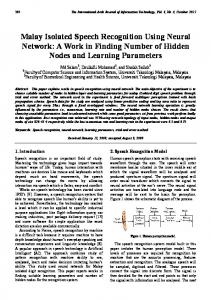
Fig. 1: Proposed DNN-based speech enhancement system. Both the single-channel and the multichannel versions are shown. ate simulated feature sequences according to this distribution. In addition, we evaluate the benefit of feature transforms [18– 20] and recurrent neural network (RNN) based language modeling [21] in combination with context-dependent deep neural network hidden Markov model (CD-DNN-HMM) acoustic modeling [22] in the context of the CHiME-3 Challenge. The rest of this paper is organized as follows. Sections 2 and 3 describe the speech enhancement system and the feature simulation method, respectively. Section 4 presents the experimental setups and results. Finally, Section 5 concludes the paper. 2. DNN-BASED MULTICHANNEL SPEECH ENHANCEMENT 2.1. Problem formulation Following classical source separation terminology [6], let us denote by I the number of channels, J the number of sources, x(t) the observed multichannel mixture signal, and cj (t) the multichannel spatial image of the j-th source. In the context of the CHiME-3 Challenge, the mixture is a noisy speech signal with I = 6 channels and J = 2 sources, namely speech and noise. This mixture signal can be expressed as x(t) =

J X

cj (t).

(1)

j=1

The I × 1 vector cj (f, n) of complex STFT coefficients of cj (t) in time frame n and frequency bin f is assumed to follow a multivariate zero-mean Gaussian distribution [23,24] cj (f, n) ∼ N (0, vj (f, n)Rj (f ))

(2)

where vj (f, n) is the power spectral density (PSD) of the j-th source for time-frequency bin (f, n) and Rj (f ) is its I × I spatial covariance matrix for frequency bin f .

Given this model, source separation can be addressed by estimating the PSDs vbj (f, n) and the spatial covariance mab j (f ) of all sources and deriving the estimated source trices R images b cj (f, n) in the minimum mean square error (MMSE) sense using multichannel Wiener filtering [6]. Finally, b cj (t) is recovered from b cj (f, n) by inverse STFT. 2.2. Proposed framework The proposed DNN-based separation framework is depicted in Fig. 1. It consists of three main successive steps. First, the channels of the input noisy signal are aligned according to the estimated time difference of arrival (TDOA). Second, the PSDs of speech and noise are estimated using a DNN. Third, the spatial covariance matrices of speech and noise are estimated and used to derive the multichannel spatial image of speech which is finally downmixed into a single channel signal. A single-channel variant of this framework which boils down to the approach in [13] is also depicted for comparison. We describe each step in detail in the following.

2.2.1. Channel alignment In the first step, we measure the time-varying TDOAs between the speaker’s mouth and each of the microphones using the provided baseline speaker localization tool [4], which relies on a nonlinear variant of SRP-PHAT [25,26]. All channels are then aligned with each other by shifting the phase of the STFT x(f, n) of the input noisy signal x(t) in all timefrequency bins (f, n) by the opposite of the measured delays. This preprocessing is required to satisfy the model in (2) which assumes that the sources do not move over time. In addition, we obtain a single-channel signal by averaging the realigned channels together. The combination of time alignment and channel averaging is known as DS beamforming in the microphone array literature [5].

2.2.2. Estimation of the source spectra In the second step, we estimate the PSDs vbj (f, n) of speech and noise using a DNN. This usage of DNNs is similar to the one in [9–11] with a few improvements detailed below. DNN architecture The DNN follows a multilayer perceptron architecture. The activation functions of the hidden layers and the output layer are rectified linear unit (ReLU) [27] and linear activation functions, respectively. DNN input and output The DNN maps input noisy speech spectra into output speech and noise spectra. Following [13], these spectra are magnitude STFT spectra aj (f, n) computed from single-channel signals after DS beamforming. They are related to the PSDs by the equation vj (f, n) = a2j (f, n). The input frames are concatenated into supervectors consisting of a center frame, left context frames, and right context frames. In choosing the context frames, we use every second frame relative to the center frame in order to reduce the redundancies caused by the windowing of STFT. Although this causes some information loss, this enables the supervectors to represent a longer context [28, 29]. In addition, we do not use the feature values of context frames directly, but the difference between the values of the context frames and the center frame. These values act as complementary features similar to delta features in the Mel frequency cepstral coefficient (MFCC) domain. The dimension of the supervectors is reduced by principal component analysis (PCA) to the dimension of the DNN input. Standardization (zero mean, unit variance) is done element-wise before and after PCA over the training data as in [30]. The output is also standardized element-wise over the training data1 . The standardization factors and the PCA transformation matrix are then kept for pre-processing and postprocessing for any input and output. In addition, a flooring function is employed at the end of post-processing so that the final output is nonnegative. DNN training The loss function used for training is the sum of the mean square error (MSE) and an L2 regularization term X λX 2 1 (b aj (f, n) − aj (f, n))2 + wk L= 2JF N 2 j,f,n

(3)

The DNNs are trained by greedy layer-wise supervised training [31] where the hidden layers are added incrementally. Training is done by backpropagation with adaptive learning rate and minibatch. The learning rate is updated following the algorithm in [32], which is driven by the validation error of previous epochs. When several training iterations have failed to get better parameters, the algorithm reverts to the last best parameters (weights and biases). While the original algorithm uses only the maximum number of epochs as the stopping criterion, we added the maximum number of reversions called patience as an early-stopping criterion. Nesterov’s accelerated gradient (NAG) is used for updating the weights instead of standard stochastic gradient descent with classical momentum (SGD-CM) as NAG behaves more stably in many situations [33]. 2.2.3. Multichannel filtering and downmixing In the third step, given the estimated PSDs of speech and noise, the spatial covariance matrices of speech and noise are estimated using the iterative procedure in [34] that is a computational simplification of the exact expectation-maximization (EM) algorithm in [35]. This iterative procedure can be divided into separation and fitting steps. In the separation step, given the estimated parameters b j (f ) of all sources, the source spatial image vbj (f, n) and R estimates b cj (f, n) are obtained by multichannel Wiener filtering. We use the following regularized variant of multichannel Wiener filtering:  −1 b c (f, n) R b x (f, n) + δII b cj (f, n) = R x(f, n) j

(4)

b c (f, n) = vbj (f, n)R b j (f ) is the source covariance where R j P J b x (f, n) = b matrix, R j=1 Rcj (f, n) is the mixture covariance matrix, II is the I × I identity matrix and δ is the regularization coefficient. b j (f ) In the fitting step, the spatial covariance matrices R are updated given the source spatial image estimates b cj (f, n) as follows: b j (f ) ← R

N X n=1

!−1 vbj (f, n)

N X

b cj (f, n)b cj (f, n)H .

(5)

n=1

k

where F is the number of frequency bins, N is the total number of time frames, b aj (f, n) are the estimated outputs, aj (f, n) are the training targets, λ is the regularization parameter, and wk are the DNN weights. No regularization is applied to the biases. 1 Properly speaking, the standardization of the output is not element-wise but frequency-bin-wise, because the computation of standardization factors for frequency bin f considers all data of frequency bin f from the two target sources (speech and noise). This was done to maintain the ratio between each source in the standardized feature space.

These two steps are repeated for L iterations after initialb j (f ) to the identity matrix. Finally, the average of izing R the channels of b cj (t) is computed, so as to achieve further enhancement and obtain a single-channel signal. Interestingly, the conventional EM approach [34, 35] upb j (f ) but also vbj (f, n) so that its estimation is dates not only R refined at every iteration. We tried this idea using additional DNNs in place of the EM updates but the preliminary experiments showed that it did not provide any improvement in the context of CHiME-3.

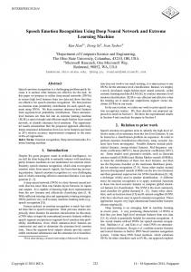
Fig. 2: CRBM topology 3. CRBM-BASED DATA SIMULATION After replacing the provided baseline enhancement technique by the provided technique, the difference in ASR performance between simulated and real data decreased but remained significant, as we shall see in Section 4. This motivated us to improve the data simulation baseline so as to increase the match between real and simulated data after enhancement. Given the large dimensionality of time domain signals and the limitations of time-domain simulation outlined in Section 1, we conduct this simulation in the feature domain. Our approach is based on the concept of CRBM, which was previously employed for, e.g., human motion modeling [17], speech synthesis [36], and voice conversion [37]. More precisely, we employ a CRBM to learn the distribution of enhanced speech features given ground truth speech and noise features. 3.1. CRBM Restricted Boltzmann machines (RBMs) [38] are generative models that learn the probabilistic distribution of input data in an unsupervised manner. In our work, the objective is to learn a conditional distribution. CRBMs achieve this goal by adding two directed connections in addition to the undirected connections in the RBM, as illustrated in Fig. 2. The first directed connection links the condition data to the visible layer and the second directed connection links the condition data to the hidden layer. Given the condition data, the visible layer and the hidden layer form an RBM whose parameters depend on the condition data. Denoting by x ∈ RΓ the condition data, y ∈ RV the data whose conditional distribution needs to be modeled and h ∈ {0, 1}H the vector of hidden neuron values, the energy function of the CRBM can be written as [36] P V X (yi − ai − k Aki xk )2 ψ(y, h, x; λ) = − 2σi2 i=1 −

H V X H X X X yi (bj + Bkj xk )hj − wij hj . (6) σ i j=1 i=1 j=1 k

Here σi are standard deviation parameters which are commonly fixed to a predetermined value, A ∈ RΓ ×V and a ∈ RV are the weights and biases of the visible layer, B ∈ RΓ ×H

Fig. 3: Training the CRBM.

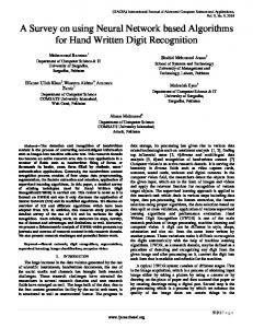
Fig. 4: Obtaining simulated feature vectors using CRBM. and b ∈ RH are the weights and biases of the hidden layer, and λ = {A, B, a, b}. The conditional distribution of y given x can be seen as a Gaussian mixture model (GMM) with 2H components X p(y|x, λ) = p(y, h|x, λ) (7) h

=

1 X exp{−ψ(y, h, x; λ)} Zλ

(8)

h

where Zλ =

Z X

exp{−ψ(y, h, x; λ)}dy.

(9)

h

CRBMs are trained using the contrastive divergence (CD) algorithm in a similar way as RBMs. 3.2. Using CRBM to simulate feature sequences We train a CRBM on the real training and development sets after applying the speech enhancement algorithm in Section 2 and use it to generate simulated training and development sets. Following CHiME-3 rules, each speech signal is associated with the corresponding original noise instance. The obtained simulated sets and the original simulated sets are then jointly used to train the ASR backend. The training and generation steps are illustrated in Fig. 3 and 4, respectively. The features consist of 13 MFCCs for each frame of clean speech (c), noise (n), and enhanced speech (e)2 . The condi2 For

clean speech and noise, channel 5 only is used.

tion data are spliced using 5 left and 5 right context frames to form supervectors n and c. These vectors along with the enhanced feature history of 5 frames (e) are concatenated to form the condition data. The distortion d = e − c of enhanced speech w.r.t. clean speech is considered as visible data. The CRBM therefore models the conditional distribution p(d|n, c, e). The simulated enhanced features are computed by adding the simulated speech distortion back to the MFCCs of clean speech. 4. EXPERIMENTS 4.1. Task and dataset We evaluated our approach in the context of the CHiME-3 Challenge in which 6-channel microphone array data in 4 varied noise settings (cafe, street junction, public transport and pedestrian area) are available. The provided data include training, development, and test sets. Each set consists of real and simulated data. The training set consists of 1,600 real and 7,138 simulated utterances, the development set consists of 1,640 real and 1,640 simulated utterances, while the test set consists of 1,320 real and 1,320 simulated utterances. The utterances are taken from the 5k vocabulary subset of the Wall Street Journal corpus [39]. All data are sampled at 16 kHz. For further details, please refer to [4]. 4.2. Algorithm settings The ground truth speech and noise signals, which are employed as training targets for DNN-based speech enhancement and as condition data for CRBM-based training and development data simulation, were extracted using the provided baseline simulation tool [4]. Note that the ground truths for real data are not perfect because they are extracted based on an estimation of the impulse responses. 4.2.1. Speech enhancement For speech enhancement, the STFT coefficients were extracted using a Hamming window of length 1024 and hopsize 512. The supervectors were built from 5 frames (2 left context, 1 center, and 2 right context frames). The DNN has an input layer size of 513, three hidden layers with a size of 1026, and an output layer size of 1026. It was trained either on the real training set only or on both the real and simulated training sets. The weights for the hidden layers were initialized randomly from apzero-mean Gaussian distribution with standard deviation of 2/nl , where nl is the number of layer inputs [40]. The weights for the output layer were initialized randomly from a zero-mean Gaussian distribution with standard deviation of 0.01. Finally, the biases were initialized to zero. The key hyper-parameters of training include the regularization coefficient λ, the minibatch size, the initial learning rate,

the decrement rate of the learning rate, the increment rate of the learning rate, the momentum, the maximum number of iterations, the maximum number of iterations before reversion, and the patience, which were set to 10−5 , 100, 10−3 , 0.7, 1.1, 0.9, 250, 5, and 3, respectively. Two variants of the algorithm were considered: the multichannel (MC) version described in Section 2 and a singlechannel (SC) version where the PSDs of speech and noise are used to compute a single-channel Wiener filter which is applied to the DS beamforming output, as shown in Fig. 1. The same DNN was used in either case. The regularization coefficient δ and the number of iterations L were set to 10−9 and 3, respectively. 4.2.2. Data simulation For data simulation, MFCCs were computed using a window size of 25 ms with a window shift of 10 ms. The visible layer of the CRBM is of dimension 13. The dimension of the condition data is 13×11×2+13×5 = 351. The number of units in the hidden layer is 2048. Each unit in the hidden layer has a sigmoid activation function. 30 iterations of Gibbs sampling were used for training and for sample generation. 4.2.3. ASR Features For ASR, MFCCs were computed as above. The 13 dimensional MFCC features were spliced with a context size of 3 frames on either side. The spliced features were decorrelated using linear discriminant analysis (LDA) [18] followed by maximum likelihood linear transform (MLLT) [19]. The transformed features were speaker normalized using feature-space maximum likelihood regression (fMLLR) [20]. The resulting feature vectors has a dimension of 40. These 40-dimensional fMLLR features along with 5 left and 5 right context frames were concatenated to form 440 dimensional supervectors, which were given as inputs to the acoustic model. Similar feature computation methods have been shown to yield best performance while training CD-DNNHMM acoustic models [41]. These features differ from the provided ASR baseline, which used spliced 40 dimensional filterbank coefficients as input features instead. Acoustic and language models The acoustic model is an 8-layer CD-DNN-HMM [22]. The 7 hidden layers have sigmoid activation functions, while the output layer uses softmax. Each hidden layer contains 2048 neurons. The total number of output senones is 1981. The total number of parameters amounts to 3.0 × 107 . To train the CD-DNN-HMM, GMM-HMM acoustic models were first trained in order to obtain state level alignments of the training data and decide the total number of senones. The CD-DNN-HMM was then trained using the cross entropy (CE) criterion followed by 4 iterations of the state-level minimum Bayes risk (sMBR) criterion [42].

Table 1: Baseline average WERs (%) on noisy data. Acoustic model GMM-HMM CD-DNN-HMM+sMBR

Dev Real Simu 18.70 18.71 16.13 14.30

Test Real Simu 33.23 21.59 33.43 21.51

The provided baseline trigram language model was used for decoding. The resulting lattices were rescored using an RNN-based language model [21] trained on the official WSJ0 data only. 4.3. Results Table 1 recalls the word error rate (WER) achieved using the CHiME-3 baseline tools. The enhancement tool is not used since it degrades results on real data. The performance of various speech enhancement techniques is compared in Table 2 using the GMM-HMM backend retrained on enhanced data. The proposed DNN-based multichannel speech enhancement technique trained on real data decreases the WER on the real test set by 39% relative compared to the baseline enhancement tool and by 23% relative compared to DS beamforming. Interestingly, single-channel enhancement (after DS beamforming) did not improve performance compared to DS beamforming alone, which indicates that proper exploitation of multichannel information is crucial. Also, the use of both real and simulated training data decreases the performance quite significantly compared to the use of real training data only, which further confirms the fact that the characteristics of simulated data do not match those of real data, even after DS beamforming. The effects of the ASR backend, CRBM-based data simulation, and RNN-based rescoring are reported in Table 3. In the first line, the CD-DNN-HMM backend trained using LDA, MLLT, and fMLLR is shown to further reduce the WER by 34% relative compared to the GMM-HMM backend. Finally, in the last line, RNN-based rescoring reduces the WER by 15% relative down to a final WER of 11.33% absolute on the real test set. The total WER reduction w.r.t. the challenge baseline amounts to 66% relative. Interestingly, CRBM data simulation slightly improves performance before RNN-based rescoring but it does not make any difference afterwards. Therefore, although we did not employ in our final challenge submission, we see it as a promising technique which deserves further investigation. The ASR performance of our best setup is detailed in Table 4 for different environments.

Table 2: Average WERs (%) for various speech enhancement methods trained on different data (GMM-HMM backend). Method and training data SC (real+simu) SC (real) DS beamforming MC (real+simu) MC (real)

Dev Real Simu 15.71 14.23 13.79 13.44 13.92 13.62 12.61 10.55 11.25 9.59

Test Real Simu 30.43 21.79 26.54 20.21 26.30 21.14 25.82 13.85 20.17 12.36

Table 3: Average WERs (%) for CRBM-based data simulation and/or RNN-based rescoring (MC (real) enhancement + fMLLR features + CD-DNN-HMM+sMBR backend). CRBM-based data simulation is used in conjunction with the simulated data provided by the CHiME3 dataset. CRBM simulation No Yes Yes No

RNN rescoring No No Yes Yes

Dev Real Simu 7.23 6.06 6.75 5.76 5.63 4.73 5.58 4.69

Test Real Simu 13.38 7.62 12.82 7.56 11.39 6.13 11.33 6.19

Table 4: Final WERs (%) for each noise condition (MC (real) enhancement + fMLLR features + CD-DNN-HMM+sMBR backend + RNN-based rescoring). Environment BUS CAF PED STR

Dev Real Simu 6.83 3.81 5.56 5.88 3.89 3.98 6.25 5.27

Test Real Simu 15.91 4.69 9.38 6.82 12.78 6.28 7.49 6.72

channel source separation approach; (2) using CRBM to generate additional training data which are similar to the acoustic conditions of real noisy data; (3) training a CD-DNNHMM by minimizing the state-sequence Bayesian risk using speaker normalized features; and finally (4) rescoring the decoded lattices using a RNN-based language model. These methods yielded an overall WER improvement of 66% relative compared to the baseline. Our system ranked 4th among 25 entries. Future work will focus on improving the proposed speech enhancement and data simulation approaches. It would also be interesting to have an integrated global optimization scheme for the iterative procedure and the DNNbased PSD estimation.

5. CONCLUSION 6. ACKNOWLEDGMENTS In this work, the following methods were used to enhance the performance of ASR in the context of the CHiME3 Challenge: (1) speech enhancement using a DNN-based multi-

We acknowledge the support of Bpifrance (FUI voiceHome), the Region Lorraine, and the CPER MISN TALC project.

7. REFERENCES [1] M. W¨olfel and J. McDonough, Distant Speech Recognition. Wiley, 2009. [2] T. Virtanen, R. Singh, and B. Raj, Eds., Techniques for Noise Robustness in Automatic Speech Recognition. Wiley, 2012. [3] L. Deng, “Front-end, back-end, and hybrid techniques for noise-robust speech recognition,” in Robust Speech Recognition of Uncertain or Missing Data - Theory and Applications. Springer, 2011, pp. 67–99. [4] J. Barker, R. Marxer, E. Vincent, and S. Watanabe, “The third ’CHiME’ speech separation and recognition challenge: Dataset, task and baselines,” in Proc. IEEE Automat. Speech Recognition and Understanding Workshop (ASRU), Scottsdale, USA, Dec. 2015, to appear. [5] K. Kumatani, J. McDonough, and B. Raj, “Microphone array processing for distant speech recognition: From close-talking microphones to far-field sensors,” IEEE Signal Process. Mag., vol. 29, no. 6, pp. 127–140, 2012. [6] E. Vincent, N. Bertin, R. Gribonval, and F. Bimbot, “From blind to guided audio source separation: How models and side information can improve the separation of sound,” IEEE Signal Process. Mag., vol. 31, no. 3, pp. 107–115, 2014. [7] L. Deng and D. Yu, “Deep learning: Methods and applications,” Found. Trends Signal Process., vol. 7, no. 3-4, pp. 197–387, Jun. 2014. [8] F. Weninger, H. Erdogan, S. Watanabe, E. Vincent, J. Le Roux, J. R. Hershey, and B. Schuller, “Speech enhancement with LSTM recurrent neural networks and its application to noise-robust ASR,” in Proc. 12th Int’l Conf. on Latent Variable Analysis and Signal Separation (LVA/ICA), Liberec, Czech Republic, Aug. 2015. [9] Y. Tu, J. Du, Y. Xu, L. Dai, and C.-H. Lee, “Speech separation based on improved deep neural networks with dual outputs of speech features for both target and interfering speakers,” in Proc. Int’l. Symp. Chinese Spoken Language Process. (ISCSLP), Sept 2014, pp. 250–254. [10] P.-S. Huang, M. Kim, M. Hasegawa-Johnson, and P. Smaragdis, “Deep learning for monaural speech separation,” in Proc. IEEE Int’l Conf. Acoust. Speech Signal Process. (ICASSP), Florence, Italy, May 2014, pp. 1562–1566. [11] ——, “Joint optimization of masks and deep recurrent neural networks for monaural source separation,” IEEE Trans. Audio, Speech, Lang. Process., vol. 23, no. 12, pp. 2136–2147, Dec. 2015.

[12] A. Narayanan and D. Wang, “Ideal ratio mask estimation using deep neural networks for robust speech recognition,” in Proc. IEEE Int’l Conf. Acoust. Speech Signal Process. (ICASSP), Vancouver, Canada, May 2013, pp. 7092–7096. [13] F. Weninger, J. Le Roux, J. R. Hershey, and B. Schuller, “Discriminatively trained recurrent neural networks for single-channel speech separation,” in Proc. IEEE Global Conf. Signal and Information Process. (GlobalSIP), Dec. 2014, pp. 577–581. [14] H.-G. Hirsch and D. Pearce, “The Aurora experimental framework for the performance evaluation of speech recognition systems under noisy conditions,” in Proc. ISCA Tutorial and Research Workshop ASR2000 — Automatic Speech Recognition: Challenges for the new Millenium, Paris, France, Aug. 2000. [15] E. Vincent, J. Barker, S. Watanabe, J. Le Roux, F. Nesta, and M. Matassoni, “The second ‘CHiME’ speech separation and recognition challenge: Datasets, tasks and baselines,” in Proc. IEEE Int’l Conf. Acoust. Speech Signal Process. (ICASSP), Vancouver, Canada, 2013, pp. 126–130. [16] L. Cristoforetti, M. Ravanelli, M. Omologo, A. Sosi, A. Abad, M. Hagm¨uller, and P. Maragos, “The DIRHA simulated corpus,” in Proc. Language Resources and Evaluation Conf. (LREC), 2014, pp. 2629–2634. [17] G. W. Taylor, G. E. Hinton, and S. T. Roweis, “Modeling human motion using binary latent variables,” in Proc. Conf. on Neural Information Processing Systems (NIPS), Vancouver, Canada, Dec. 2006, pp. 1345–1352. [18] R. O. Duda, P. E. Hart, and D. G. Stork, Pattern classification. John Wiley & Sons, 2012. [19] R. A. Gopinath, “Maximum likelihood modeling with Gaussian distributions for classification,” in Proc. IEEE Int’l Conf. Acoust. Speech Signal Process. (ICASSP), vol. 2, Seattle, USA, 1998, pp. 661–664. [20] M. J. Gales, “Maximum likelihood linear transformations for HMM-based speech recognition,” Computer Speech & Language, vol. 12, no. 2, pp. 75–98, 1998. [21] T. Mikolov, M. Karafi´at, L. Burget, J. Cernock´y, and S. Khudanpur, “Recurrent neural network based language model.” in Proc. ISCA INTERSPEECH, Makuhari, Japan, Sep. 2010, pp. 1045–1048. [22] G. Hinton, L. Deng, D. Yu, G. Dahl, A. Mohamed, N. Jaitly, A. Senior, V. Vanhoucke, P. Nguyen, T. Sainath, and B. Kingsbury, “Deep neural networks for acoustic modeling in speech recognition: The shared views of four research groups,” IEEE Signal Process. Mag., vol. 29, no. 6, pp. 82–97, Nov. 2012.

[23] N. Q. K. Duong, E. Vincent, and R. Gribonval, “Underdetermined reverberant audio source separation using a full-rank spatial covariance model,” IEEE Trans. Audio, Speech, Lang. Process., vol. 18, no. 7, pp. 1830–1840, Jul. 2010. [24] A. Liutkus, D. Fitzgerald, Z. Rafii, B. Pardo, and L. Daudet, “Kernel additive models for source separation,” IEEE Trans. Signal Process., vol. 62, no. 16, pp. 4298–4310, Aug. 2014. [25] B. Loesch and B. Yang, “Adaptive segmentation and separation of determined convolutive mixtures under dynamic conditions,” in Proc. 9th Int’l Conf. on Latent Variable Analysis and Signal Separation (LVA/ICA), 2010, pp. 41–48. [26] C. Blandin, A. Ozerov, and E. Vincent, “Multi-source TDOA estimation in reverberant audio using angular spectra and clustering,” Signal Processing, vol. 92, no. 8, pp. 1950–1960, 2012. [27] X. Glorot, A. Bordes, and Y. Bengio, “Deep sparse rectifier networks,” in Proc. Int’l. Conf. Artificial Intelligence and Statistics (AISTATS), vol. 15, Fort Lauderdale, USA, Apr. 2011, pp. 315–323. [28] A. A. Nugraha, K. Yamamoto, and S. Nakagawa, “Single-channel dereverberation by feature mapping using cascade neural networks for robust distant speaker identification and speech recognition,” EURASIP J. Audio, Speech and Music Process., vol. 2014, no. 13, 2014. [29] S. Uhlich, F. Giron, and Y. Mitsufuji, “Deep neural network based instrument extraction from music,” in Proc. IEEE Int’l Conf. Acoust. Speech Signal Process. (ICASSP), Brisbane, Australia, Apr. 2015, pp. 2135– 2139. [30] X. Jaureguiberry, E. Vincent, and G. Richard, “Fusion methods for audio source separation,” Dec. 2014. [Online]. Available: https://hal.archives-ouvertes.fr/ hal-01120685 [31] Y. Bengio, P. Lamblin, D. Popovici, and H. Larochelle, “Greedy layer-wise training of deep networks,” in Proc. Conf. on Neural Information Processing Systems (NIPS), Vancouver, Canada, Dec. 2006, pp. 153–160. [32] S. Duffner and C. Garcia, “An online backpropagation algorithm with validation error-based adaptive learning rate,” in Proc. Int’l. Conf. Artificial Neural Networks (ICANN), Porto, Portugal, Sep. 2007, pp. 249–258. [33] I. Sutskever, J. Martens, G. E. Dahl, and G. E. Hinton, “On the importance of initialization and momentum in deep learning,” in Proc. Int’l. Conf. Machine Learning (ICML), Atlanta, USA, Jun. 2013, pp. 1139–1147.

[34] A. Liutkus, D. Fitzgerald, and Z. Rafii, “Scalable audio separation with light kernel additive modelling,” in Proc. IEEE Int’l Conf. Acoust. Speech Signal Process. (ICASSP), Brisbane, Australia, Apr. 2015, pp. 76–80. [35] A. Ozerov, E. Vincent, and F. Bimbot, “A general flexible framework for the handling of prior information in audio source separation,” IEEE Trans. Audio, Speech, Lang. Process., vol. 20, no. 4, pp. 1118–1133, May 2012. [36] Z.-H. Ling, S.-Y. Kang, H. Zen, A. Senior, M. Schuster, X.-J. Qian, H. Meng, and L. Deng, “Deep learning for acoustic modeling in parametric speech generation: A systematic review of existing techniques and future trends,” IEEE Signal Process. Mag., vol. 32, no. 3, pp. 35–52, May 2015. [37] T. Nakashika, T. Takiguchi, and Y. Ariki, “Voice conversion in time-invariant speaker-independent space,” in Proc. IEEE Int’l Conf. Acoust. Speech Signal Process. (ICASSP), May 2014, pp. 7889–7893. [38] A. Fischer and C. Igel, “An introduction to restricted Boltzmann machines,” in Progress in Pattern Recognition, Image Analysis, Computer Vision, and Applications. Springer, 2012, pp. 14–36. [39] J. Garofalo, D. Graff, D. Paul, and D. Pallett, “CSR-I (WSJ0) Complete,” 2007, Linguistic Data Consortium, Philadelphia. [40] K. He, X. Zhang, S. Ren, and J. Sun, “Delving deep into rectifiers: Surpassing human-level performance on imagenet classification,” in Proc. Int’l. Conf. Computer Vision (ICCV), Santiago, Chile, Dec. 2015. [41] S. P. Rath, D. Povey, and K. Vesel´y, “Improved feature processing for deep neural networks.” in Proc. ISCA INTERSPEECH, Lyon, France, Aug. 2013, pp. 109–113. [42] K. Vesel´y, A. Ghoshal, L. Burget, and D. Povey, “Sequence-discriminative training of deep neural networks.” in Proc. ISCA INTERSPEECH, Lyon, France, Aug. 2013, pp. 2345–2349.