This bias can be reduced by decor- relating the incoming ...... [71] M. G. Siqueira, R. Speece, E. Petsalis, A. Alwan, S. Soli, and S. Gao, âSubband adaptive ..... [124] C. R. C. Nakagawa, S. Nordholm, and W.-Y. Yan, âDual microphone solution.
ROBUST FEEDBACK SUPPRESSION ALGORITHMS FOR SINGLE- AND M U LT I - M I C R O P H O N E H E A R I N G A I D S
Von der Fakultät für Medizin und Gesundheitswissenschaften der Carl von Ossietzky Universität Oldenburg zur Erlangung des Grades und Titels eines Doktor der Ingenieurwissenschaften (Dr.-Ing.) angenommene Dissertation
von henning schepker geboren am 04.07.1986 in Bremen (Deutschland)
Henning Schepker: Robust feedback suppression algorithms for single- and multimicrophone hearing aids erstgutachter: Prof. Dr. ir. Simon Doclo, University of Oldenburg, Germany weitere gutachter: Prof. Dr. Sven Nordholm, Curtin University, Australia Prof. Dr. Jesper Jensen, Aalborg University, Denmark
tag der disputation: 19. Dezember 2017
Never lose the child-like wonder. It’s just too important. It’s what drives us. — Randy Pausch, Sep. 2007 Dedicated to my parents. Thank you for your continuous support.
ACKNOWLEDGMENTS
This thesis has been written at the Signal Processing Group in the Department of Medical Physics and Acoustics of the Carl von Ossietzky Universität Oldenburg in Oldenburg, Germany. I would like to take the opportunity to thank the many people who contributed in several ways to the completion of this work. First, I want to thank my supervisor Prof. Simon Doclo for providing me with the opportunity to write this thesis and his continuous support, his numerous ideas and suggestions. By creating an open and friendly work environment he provided the basis and the freedom to pursue my scientific interests, while still providing invaluable guidance, which can not be appreciated enough. Furthermore, I would like to thank Prof. Sven Nordholm for interesting discussion during my stays in his lab in Perth and during his visits in Oldenburg as well as reviewing this thesis. I am thankful to Prof. Jesper Jensen for reviewing my thesis participating in my thesis committee and for showing much interest in my work. Furthermore, I would like to thank Steven van de Par for participating in the thesis committee. I am grateful to Dr. Jan Rennies-Hochmuth whose early guidance in my Bachelor’s and Master’s thesis lead to my increased interest in research and an ongoing fruitful and successful collaboration on topics beyond the scope of this thesis. A special thanks also to all current and past members of the Signal Processing group. Not only did they provide a friendly and relaxed work environment, but we also made some memorable evenings with watching football, Playstation gaming, several BBQs and after conference activities like renting a house in Australia and almost getting lost in China. I want to thank all of my colleagues at the Department of Medical Physics and Acoustics, the Institute of Hearing Technology and Audiology at Jade Hochschule Oldenburg and Fraunhofer Institute of Digital Media Technology for numerous discussions and collaborations. Many thanks as well to the members of the Department of Electrical and Computer Engineering at Curtin University for the enjoyable time during my stays in Perth. I am thankful to all my friends who supported me along the path that lead to this thesis. Before missing out on someone, I keep it simple. Thank you for helping to distract and refocus, joining for numerous coffee breaks in the past years, enjoyable evenings with playstation, BBQ, beer, and whisky, climbing and bouldering, or just easy chats when things were getting tough. And to those of you who proof-read parts of this thesis, thank you!
v
Last but not least I want to thank my parents and my sister for their continuous support and encouragement. Oldenburg, June 2018 Henning Schepker
vi
ABSTRACT
When providing the necessary amplification in hearing aids, the risk of acoustic feedback is increased due to the coupling between the hearing aid loudspeaker and the hearing aid microphone(s). This acoustic feedback is often perceived as an annoying whistling or howling. Thus, to reduce the occurrence of acoustic feedback, robust and fast-acting feedback suppression algorithms are required. The main objective of this thesis is to develop and evaluate algorithms for robust and fast-acting feedback suppression in hearing aids. Specifically, we focus on enhancing the performance of adaptive filtering algorithms that estimate the feedback component in the hearing aid microphone by reducing the number of required adaptive filter coefficients and by improving the trade-off between fast convergence and good steady-state performance. Additionally, we develop fixed spatial filter design methods that can be applied in a multi-microphone earpiece. The main contributions of this thesis are threefold. First, we propose several optimization procedures that allow to compute a fixed common pole-zero filter from multiple measured acoustic feedback paths, effectively allowing to reduce the number of adaptive filter coefficients. Second, we propose an affine combination of two adaptive filters with different step-sizes to overcome the limitations associated with a single fixed step-size. Third, we propose several optimization procedures to design a robust fixed null-steering beamformer that can be used for acoustic feedback suppression in a multi-microphone earpiece and can be combined with an adaptive filter to reduce the residual feedback component in the beamformer output. In order to reduce the number of adaptive filter coefficients in adaptive feedback cancellation, we propose several optimization procedures to estimate a common pole-zero filter from multiple measured acoustic feedback paths. The proposed optimization procedures aim either at minimizing the misalignment or at maximizing the maximum stable gain. To ensure the stability of the common pole-zero filter, we propose to use two different constraints. The first constraint is based on the positive realness of the frequency-response of the all-pole component of the common pole-zero filter, while the second constraint is based on Lyapunov theory. The resulting constrained optimization problems to estimate the common pole-zero filter can either be formulated as a linear programming problem, a quadratic programming problem or a semidefinite programming problem. Simulation results using measured acoustic feedback paths from a two-microphone behind-the-ear hearing aid show that the proposed common pole-zero filter outperforms the existing common all-pole and common all-zero filter. Furthermore, results show that for a desired misalignment or maximum stable gain the number of adaptive filter coefficients can be robustly reduced. When implemented in a state-of-the-art adaptive feedback
vii
cancellation algorithm, using the common pole-zero filter allows to increase the convergence speed. In order to improve the trade-off between fast convergence and good steady-state performance, we propose to use an affine combination of two adaptive filters with different step-sizes. The first adaptive filter uses a large step-size, leading to a fast convergence but large steady-state misalignment, while the second adaptive filter uses a small step-size, leading to a slow convergence but low steady-state misalignment. The proposed affine combination of these two filters then exhibits the fast convergence properties of the first filter and the low steady-state misalignment of the second filter. We theoretically show that the optimal combination parameter is biased when the loudspeaker signal and the incoming signal are correlated. In order to reduce this bias, we propose to use the prediction-error-method and present a time-domain and a frequency-domain implementation. Simulations using measured acoustic feedback paths show the improved convergence speed and low steady-state misalignment of the proposed affine combination compared to a system utilizing only a single fixed step-size. Finally, we propose different optimization procedures to obtain a fixed null-steering beamformer for a multi-microphone earpiece. The proposed optimization procedures aim either at minimizing the residual feedback power or maximizing the maximum stable gain. In order to avoid the trivial solution, we propose two different constraints. The first constraint sets the beamformer coefficients in a reference microphone to be a delay, while the second constraint aims at preserving the relative transfer function of the incoming signal. In order to allow for a trade-off between distortions of the incoming signal and acoustic feedback cancellation performance, we further propose to incorporate the relative transfer function constraint as a soft constraint. To improve the robustness of the null-steering beamformer to variations of the acoustic feedback paths, we propose to incorporate multiple sets of acoustic feedback path measurements. The resulting constrained optimization problems to compute the null-steering beamformer can be formulated as a least-squares problem with closed-form solution, a linear programming problem, a quadratic programming problem with quadratic constraints or a semidefinite programming problem. Results using measured acoustic feedback paths from a custom multi-microphone earpiece show that the fixed null-steering beamformer allows to robustly increase the added stable gain of the multi-microphone earpiece by more than 50 dB without significantly distorting the incoming signal. Furthermore, when combined with an adaptive filter to cancel the residual feedback component in the beamformer output, the performance can be further increased, where the performance of the null-steering beamformer and the adaptive filter are approximately complementary.
viii
ZUSAMMENFASSUNG
Nach aktuellen Schätzungen steigt die Anzahl an hörgeschädigten Personen stetig an. Häufig führt die Hörschädigung zu einem verringerten Sprachverstehen in herausfordernden akustischen Situation wie z. B. in Besprechungen und der sozialen Interaktion in lauten Umgebungen. Dies macht die Nutzung von Hörgeräten unumgänglich. Um ein normales Hörvermögen wieder herzustellen ist häufig eine hohe Verstärkung notwendig. Diese erhöht das Auftreten von Rückkopplungen durch die akustische Kopplung zwischen Hörgerätelautsprecher und Hörgerätemikrofon. Diese akustischen Rückkopplungen werden häufig als störendes Pfeifen oder Heulen wahrgenommen. Um die akustischen Rückkopplungen zu unterdrücken sind daher robuste und schnell agierende Rückkopplungsunterdrückungsalgorithmen notwendig. Das Hauptziel dieser Arbeit ist es daher robuste und schnell agierende Algorithmen zur akustischen Rückkopplungsunterdrückung in Hörgeräten zu entwickeln und zu untersuchen. Im speziellen liegt der Fokus auf der Verbesserung von Algorithmen basierend auf adaptiven Filtern welche die Rückkopplungskomponente im Hörgerätemikrofon schätzen. Das Ziel ist hierbei die Reduktion der notwendigen Anzahl an adaptiven Filterkoeffizienten und die Verbesserung des Kompromisses zwischen schneller Konvergenz und guter Leistung während des stationären Verhaltens. Ein weiteres Ziel ist die Entwicklung von Optimierungsverfahren zum Entwurf von festen räumlichen Filtern zur akustischen Rückkopplungsunterdrückung in einem Ohrstück mit mehreren Mikrofonen. Diese Arbeit hat drei Hauptbeiträge. Als erstes werden mehrere Optimierungsverfahren vorgeschlagen, um ein festes gemeinsames Pol-Nulstellen Filter aus mehreren gemessenen akustischen Rückkopplungspfaden zu schätzen, welches es erlaubt die Anzahl der adaptiven Filterkoeffizienten zu reduzieren. Als zweites wird die affine Kombination von zwei adaptiven Filtern mit unterschiedlichen Schrittweiten vorgeschlagen, um die Limitierung einer einzelnen festen Schrittweite zu umgehen. Als drittes werden mehrere Optimierungsverfahren vorgeschlagen, um ein festes robustes räumliches Nullstellenfilter zur akustischen Rückkopplungensunterdrückung zu entwerfen. Dieses räumliche Filter wird weiterhin mit einem adaptiven Filter kombiniert, welches die residuale Rückkopplungskomponente im Ausgang des räumlichen Filters reduziert. Um die Anzahl der adaptiven Filterkoeffizienten bei der adaptiven Rückkopplungsunterdrückung zu reduzieren, werden mehrere Optimierungsverfahren vorgeschlagen, um ein festes gemeinsames Pol-Nullstellenfilter aus mehreren gemessenen akustischen Rückkopplungspfaden zu schätzen. Die vorgeschlagenen Optimierungsverfahren minimieren entweder die quadratische Abweichung des PolNullstellenfilters vom akustischen Rückkopplungspfad oder die maximale stabile
ix
Verstärkung des Hörgeräts. Um die Stabilität des gemeinsamen Pol-Nullstellenfilters zu gewährleisten, werden zwei unterschiedliche Nebenbedingungen für die Optimierung vorgeschlagen. Die erste Nebenbedingung basiert auf der positiven Reellwertigkeit der Frequenzantwort des All-Pol Anteils des Pol-Nullstellenfilters, während die zweite Nebenbedingung auf der Lyapunovtheorie basiert. Bei der Nutzung der ersten Nebenbedingung, basierend auf der positiven Reellwertigkeit der Frequenzantwort des All-Pol Anteils, wird das Optimierungsproblem zur Schätzung des gemeinsamen Pol-Nullstellenfilters entweder als quadratisches Programm zur Minimierung der quadratischen Abweichung oder als lineares Programm unter Benutzung des Reellen-Rotationstheorems zur Maximierung der maximalen stabilen Verstärkung formuliert. Bei der Nutzung der zweiten Nebenbedingung, basierend auf der Lyapunovtheorie, wird in beiden Fällen das Optimierungsproblem als semidefinites Programm formuliert. Simulationen mit gemessenen akustischen Rückkopplungspfaden von einem zwei-Mikrofon hinter-dem-Ohr Hörgerät zeigen, dass das gemeinsame PolNullstellenfilter eine bessere Leistung erzielt als das existierenden gemeinsame Polstellenfilter und das gemeinsame Nullstellenfilter. Weiterhin erlaubt das gemeinsame Pol-Nullstellenfilter die robuste Reduktion der Anzahl an adaptiven Parametern des adaptiven Filters. Bei der Anwendung des gemeinsamen Pol-Nullstellenfilters in einem adaptiven Rückkopplungsunterdrückungsalgorithmus zeigt sich im Vergleich zu einem adaptiven Algorithmus, welcher kein festes gemeinsames Filter benutzt, eine erhöhte Konvergenzgeschwindigkeit. Um den Kompromiss zwischen schneller Konvergenz und guter Leistung während des stationären Verhaltens von adaptiven Filtern zu vereinfachen, wird die affine Kombination von zwei adaptiven Filtern mit unterschiedlichen Schrittweiten vorgeschlagen. Während das erste Filter eine große Schrittweite nutzt und zu einer schnellen Konvergenz, aber eine schlechtere stationäre Leistung aufweist, nutzt das zweite Filter eine kleinere Schrittweite und hat somit eine langsamere Konvergenz, aber eine bessere stationäre Leistung. Die affine Kombination dieser beiden Filter übernimmt schließlich die schnelle Konvergenz des ersten Filters und die gute stationäre Leistung des zweiten Filters. Simulationen mit gemessenen akustischen Rückkopplungspfaden zeigen die Verbesserung bei der Nutzung der affinen Kombination gegenüber einem System mit nur einer festen Schrittweite. Schließlich werden verschiedene Optimierungsverfahren vorgeschlagen, um ein robustes festes räumliches Nullstellenfilter für ein Ohrstück mit zwei Mikrofonen und einem Lautsprecher in der Belüftungsbohrung und einem dritten Mikrofon in der Concha zu entwerfen. Die Optimierungsverfahren minimieren entweder die quadratische Leistung am Ausgang des räumlichen Filters oder die maximale stabile Verstärkung des Ohrstücks. Um die Triviallösung zu vermeiden werden zwei unterschiedliche Nebenbedingungen für die Optimierung vorgeschlagen und untersucht. Bei der ersten Nebenbedingung werden die Koeffizienten in einem Referenzmikrofon als Verzögerung angenommen. Bei der zweiten Nebenbedingung wird die relative Übertragungsfunktion für das eintreffende Signal bewahrt. Um einen Kompromiss zwischen Verzerrungen im eintreffenden Signal und der Rückkopplungsunterdrückung zu erlauben, wird weiterhin vorgeschlagen die Nebenbedingung basierend auf
x
der relativen Übertragungsfunktion als zusätzlichen Term in die Kostenfunktion zu übernehmen. Ergebnisse basierend auf Simulationen mit gemessenen akustischen Rückkopplungspfaden des Ohrstücks mit mehreren Mikrofonen zeigen, dass die maximale stabile Verstärkung robust um mehr als 50 dB erhöht werden kann ohne das eintreffende Signal signifikant zu verzerren. Weiterhin zeigen Ergebnisse mit der zusätzlichen Nutzung eines adaptiven Filters zur Unterdrückung der residualen Rückkopplungskomponente im Ausgang des räumlichen Filters, dass die Leistungsfähigkeit mit der Kombination weiter erhöht werden kann und die Leistung des räumlichen Filters und des adaptiven Filters komplementär sind.
xi
GLOSSARY
Acronyms AFC
adaptive feedback cancellation
ALS
alternating least-squares
ASG
added stable gain
ATF
acoustic transfer function
BTE
behind-the-ear
CAPZ
common-acoustical-pole and zero
ECLG
effective closed-loop gain
DFT
discrete Fourier transform
FIR
finite impulse response
IIR
infinite impulse response
IR
impulse response
LMI
linear matrix inequality
LMS
least mean squares
LP
linear programming
MOS
mean opinion score
MSG
maximum stable gain
NLMS
normalized least mean squares
PBFDAF
partitioned block frequency-domain adaptive filter
PEM
prediction-error-method
PESQ
perceptual evaluation of speech quality
QP
quadratic programming
QPQC
quadratic program with quadratric constraints
RTF
relative transfer function
xiii
SDP
semidefinite programming
SIMO
single-input-multiple-output
SISO
single-input-single-output
SLMM
single-loudspeaker multi-microphone
SLSM
single-loudspeaker single-microphone
SR-LMS
sign-regressor least mean squares
sSSN
stationary speech-shaped noise
Mathematical Notation a
scalar a
a
vector a
LA
length of a vector vector a
A
matrix A
a ˆ
estimate of scalar a
ˆ a
estimate of vector a
ˆ A
estimate of matrix A
aT A
T
aH A
H
transpose of vector a transpose of matrix A conjugate transpose (hermitian) of vector a conjugate transpose (hermitian) of matrix A
A−1
inverse of matrix A
ai
ith element of vector a
x[k]
discrete-time sequence at discrete-time index k
X(ω)
discrete-time Fourier transform of x[k] at continuous normalized frequency ω
X(ωn )
discrete-time Fourier transform of x[k] at discrete normalized frequency ωn
Rxx [k]
auto-correlation matrix of vector x[k]
Rxy [k]
cross-correlation matrix of vectors x[k] and y[k]
E
expectation operator
xiv
FNF F T
discrete-time Fourier transform matrix of size NF F T × NF F T
|·|
absolute value
k · k2
l2 -norm
Fixed Symbols k
discrete-time index
l
discrete block index
m
microphone index
p
partition index
q
discrete-time delay operator
ω
continuous normalized frequency
ωn
discrete normalized frequency
dG
delay in the hearing aid forward path transfer function
Ds
decimation factor of subband filterbank
LH
length of acoustic feedback path H(q, k)
LHˆ
ˆ k) length of the adaptive filter H(q,
Ls
length of subband adaptive filter
LW
number of beamformer coefficients
M
number of microphones
Ms
number of subbands
NA
order of linear prediction filter ALP (q, k)
Npc
order of all-pole part of common pole-zero filter
Nzc
order of all-zero part of common pole-zero filter
Nzh
order of acoustic feedback path
Nzv
order of variable part all-zero filter
NF F T
DFT size
Nφ
number of rotation angles
P
length of partition
e[k]
error signal
xv
ef [k]
prewhitened error signal
e˜[k]
beamformer output signal
f [k]
feedback component
ff [k]
prewhitened feedback component
fm [k]
feedback component in the mth microphone
fˆ[k]
estimated (residual) feedback component
u[k]
loudspeaker signal
uf [k]
prewhitened loudspeaker signal
w[k]
white noise sequence
x[k]
incoming signal
xf [k]
prewhitened incoming signal
xm [k]
incoming signal in the mth microphone
y[k]
microphone signal
yf [k]
prewhitened microphone signal
ym [k]
microphone signal in the mth microphone
α
regularization parameter of adaptive filter
δ
stability margin parameter
ε
threshold parameter affine combination parameter
η[k] η
opt
[k]
optimal affine combination parameter
γm
weighting parameter in the m-th microphone
λ
trade-off parameter
µ[k]
step-size parameter
τ
stability margin parameter
ξi [k]
normalized misalignment for the ith acoustic feedback path measurement
ξm
normalized misalignment in the m-th microphone
ξ¯
average normalized misalignment
Ac (·) A
LP
xvi
(q, k)
common part all-pole filter time-varying all-pole filter transfer function of linear prediction
Ai [k]
time-varying added stable gain for the ith acoustic feedback path measurement
B c (·)
common part all-zero filter
v Bm (·)
variable part all-zero filter in the mth microphone
C(·, k)
closed-loop transfer function
Dm (·, k)
acoustic transfer function of incoming signal in the mth microphone
˜ m (·, k) D
relative transfer function of incoming signal in the mth microphone
Ei [k]
effective closed-loop gain for the ith acoustic feedback path measurement
EE Em (·)
equation-error in the mth microphone
OE (·) Em
output-error in the mth microphone
W EE (·) Em
weighted equation-error in the mth microphone
G(·, k)
hearing aid forward path
H(·, k)
acoustic feedback path
Hi (·, k)
acoustic feedback path of the ith measurement
Hm (·, k)
acoustic feedback path for the mth microphone
Hm,i (·, k)
acoustic feedback path in the mth microphone of the ith measurement
ˆ c (·) H
common part filter of acoustic feedback paths
ˆ v (·) H m
variable part filter of acoustic feedback paths in the m-th microphone
JCAP Z
CAPZ least-squares cost function
JEE
equation-error-based least-squares cost function
c JEE
equation-error-based least-squares cost function of common part
v JEE
equation-error-based least-squares cost function of variable parts
JM M
output-error-based min-max cost function
JOE
output-error-based least-squares cost function
JW EE
weighted equation-error-based least-squares cost function
c JW EE
weighted equation-error-based least-squares cost function of common part
xvii
v JW EE
weighted equation-error-based least-squares cost function of variable parts
JW M M
weighted equation-error-based min-max cost function
JP EM
cost function of the PEM
JW F
cost function of the Wiener filter estimate
Mi [k]
maximum stable gain for the ith acoustic feedback path measurement
Mm
maximum stable gain in the mth microphone
¯ M
overall maximum stable gain
O(q, k)
time-varying open-loop transfer function
Wm (·, k)
spatial filter/beamformer weighting function in the mth microphone
¯ aLP [k]
coefficient vector of linear prediction filter
c
¯ a
coefficient vector of common part all-pole filter
bc
coefficient vector of common part all-zero filter
˜c
b
zero-padded coefficient vector bc
bvm
coefficient vector of variable part all-zero filter in the mth microphone
˜ vm b
zero-padded coefficient vector bvm
bv
stacked coefficient vector of variable part all-zero filters
dm
coefficient vector of Dm (q, k)
˜m d
˜ m (q, k) coefficient vector of D
ec
coefficient vector of common part equation-error
ev
coefficient vector of variable part equation-error
f [k]
feedback component vector
f(ωn )
vector of Fourier transform coefficients at frequency ωn
h[k]
coefficient vector of H(q, k)
hi [k]
coefficient vector of Hi (q, k)
hm [k]
coefficient vector of Hm (q, k)
hm,i [k]
coefficient vector of Hm,i (q, k)
ˆ opt [k] h
optimal estimate of h[k]
xviii
˜ m [k] h
zero-padded coefficient vector hm [k]
˜ h
˜m stacked vector of coefficient vectors h
ˆ h[k]
estimate of h[k]
ˆ i [k] h
estimate of hi [k]
q
vector of delay elements q
wm
beamformer coefficient vector in the mth microphone
w
stacked vector of wm
x[k]
incoming signal vector
y[k]
microphone signal vector
∆l
step-size matrix of PBFDAF algorithm
B
positive definite matrix in steepest-descent filter update
˜c B
˜c convolution matrix of coefficient vector b
ˇc B
˜c block-diagonal matrix of convolution matrices vector B
˜ vm B
˜ vm convolution matrix of coefficient vector b
˜v B
˜ vm stacked matrix of convolution matrices B
C(q, k)
time-varying close-loop transfer function vector
D(·, k)
vector of acoustic transfer functions of incoming signal
˜ k) D(·,
vector of relative transfer functions of incoming signal
˜m D
˜m convolution matrix of coefficient vector d
˜ D
˜m stacked matrix of convolution matrices D
H(·, k)
acoustic feedback path vector
Hi (·, k)
acoustic feedback path vector for the ith measurement
˜m H
˜m convolution matrix of coefficient vector h
˜ H
˜m stacked matrix of convolution matrices H
˜ P, P
positive definite matrix
W(·, k)
spatial filter/beamformer weighting function vector
Γ
diagonal weighting matrix
Γstab
stability constraint matrix of Lyapunov constraint
xix
CONTENTS
1 introduction 1 1.1 Acoustic Feedback and Hearing Aids 2 1.2 Overview of Feedback Suppression Methods 4 1.3 Feedforward Feedback Suppression 5 1.4 Adaptive Feedback Cancellation 8 1.5 Spatial Filtering based Feedback Suppression 13 1.6 Thesis Outline and Main Contributions 13 2 acoustic setup and performance measures 17 2.1 Acoustic Systems and Notation 17 2.2 Instrumental Performance Measures 24 2.3 Summary 27 3 adaptive feedback cancellation 29 3.1 Adaptive Filtering 29 3.2 Bias Analysis 32 3.3 Bias Reduction Methods 32 3.4 Summary 39 4 common part optimization for afc in hearing aids 41 4.1 Problem Formulation 44 4.2 Review of Instrumental Measures of Feedback Cancellation Performance 46 4.3 Least-squares Optimization 47 4.4 Min-max Optimization 58 4.5 Experimental Evaluation 61 4.6 Common Part based Feedback Cancellation 90 4.7 Summary 93 5 affine combination of adaptive filters for afc 97 5.1 Proposed Adaptive Feedback Cancellation Algorithm 98 5.2 Experimental Evaluation 103 5.3 Conclusion 105 6 feedback cancellation based on null-steering 107 6.1 Acoustic Scenario and Notation 109 6.2 Fixed Null-steering Beamformer Design 111 6.3 Experimental Evaluation 120 6.4 Combined Null-Steering and Adaptive Feedback Cancellation 153 6.5 Summary 156 7 conclusion & outlook 159 7.1 Conclusion 159 7.2 Suggestions for Future Research 161
xxi
xxii
contents
a appendix to chapter 4 165 a.1 Time-domain notation of equation-error optimization 165 a.2 Proof of stability of equation-error optimization 165 v a.3 Schur Complement of JW 166 MM b measurement of acoustic feedback paths 169 c real rotation theorem 173 bibliography
177
LIST OF FIGURES
Figure 1.1
Figure 1.2 Figure 1.3 Figure 1.4 Figure 1.5 Figure 1.6 Figure 2.1 Figure 2.2 Figure 3.1 Figure 3.2 Figure 4.1 Figure 4.2 Figure 4.3 Figure 4.4 Figure 4.5
Figure 4.6
Exemplary amplitude responses of two different acoustic feedback paths of a behind-the-ear hearing aid measured in free-field and with a telephone receiver in close distance. 3 Generic single-loudspeaker single-microphone closed-loop system. 3 Generic SLSM closed-loop system with a non-linearity in the forward path. 6 Generic SLSM closed-loop system with an adaptive feedback canceller. 9 Generic SLMM closed-loop system with a fixed beamformer. 13 Schematic overview of this thesis. 15 Generic single-loudspeaker single-microphone hearing aid system with feedback suppression. 20 Generic single-loudspeaker multi-microphone hearing aid system with feedback suppression. 21 Generic single-loudspeaker single-microphone hearing aid closed-loop system with an adaptive filter. 30 Single-loudspeaker single-microphone hearing aid closedloop system using the PEM for AFC. 34 System models: (a) general SIMO system and (b) approximation of the SIMO system using a common part 45 Amplitude response (top) and phase response (bottom) of IRs m = 1, 2, 3, 4 for the first ear canal setting (diameter d1 = 6 mm and length l1 = 15 mm). 65 Amplitude response (top) and phase response (bottom) of IRs m = 5, 6, 7, 8 for the first ear canal setting (diameter d1 = 6 mm and length l1 = 15 mm). 65 Amplitude response (top) and phase response (bottom) of IRs m = 9, 10, 11, 12 for the second ear canal setting (diameter d1 = 7 mm and length l1 = 20 mm). 66 Average normalized misalignment as a function of Nzv and N c = Npc + Nzc for the set of IRs m = 1, 2 when the common part is optimized using the least-squares procedures minimizing the equation-error (cf. Algorithm 3). 68 Average normalized misalignment as a function of Nzv given a fixed N c = 20. 68
xxiii
xxiv
List of Figures
Figure 4.7 Figure 4.8 Figure 4.9 Figure 4.10
Figure 4.11
Figure 4.12
Figure 4.13
Figure 4.14
Figure 4.15
Figure 4.16
Minimum number of parameters Nzv as a function of N c required to achieve an average normalized misalignment of ξ¯ = −20 dB. 69 Average normalized misalignment and overall MSG for different initializations of the common pole-zero filter using the set of feedback paths m = 1, 2 (Npc = 12, Nzc = 4). 71 Amplitude response of H1 (f ) and amplitude responses of the residual output-errors for all three least-squares optimization procedures (Npc = 8, Nzc = 4, Nzv = 12). 73 Average normalized misalignment for the least-squares optimization procedures as a function of Nzv for different choices of Npc and Nzc for two sets of free-field IRs (m = 1, 2 top row; m = 9, 10 bottom row). 74 Overall MSG for the least-squares optimization procedures as a function of Nzv for different choices of Npc and Nzc for two sets of free-field IRs (m = 1, 2 top row; m = 9, 10 bottom row). 75 Location of the poles for Npc = 8, Nzc = 0, Nzv = 12 for the set of IRs m = 1, 2 using the equation-error based optimization procedure (without constraints) and when using the equation-error based optimization procedure with stability constraints on the pole locations (QP: positive realness stability constraint; SDP: Lyapunov stability constraint). 75 Minimum average normalized misalignment for the leastsquares optimization procedure using the Lyapunov stability constraint as a function of Nzv for different choices of N c for the set of IRs m = 1, 2. 76 Maximum overall MSG for the least-squares optimization procedure using the Lyapunov stability constraint as a function of Nzv for different choices of N c for the set of IRs m = 1, 2. 77 Minimum average normalized misalignment for the leastsquares optimization procedure using the Lyapunov stability constraint as a function of Nzv for different unknown acoustic feedback paths and number of common part parameters N c . The common part was estimated from the free-field IRs m = 1, 2. 78 Maximum overall MSG for the least-squares optimization procedure using the Lyapunov stability constraint as a function of Nzv for different unknown acoustic feedback paths and number of common part parameters N c . The common part was estimated from the free-field IRs m = 1, 2. 79
List of Figures
Figure 4.17
Figure 4.18
Figure 4.19
Figure 4.20
Figure 4.21
Figure 4.22
Figure 4.23
Figure 4.24
Figure 4.25
Minimum number of required variable part parameters Nzv for the least-squares optimization procedure using the Lyapunov stability constraint as a function of required common part parameters N c to obtain a desired average normalized misalignment of (left) -30 dB, (middle) -20 dB and (right) -10 dB for different acoustic feedback paths. The common part was estimated from the set of free-field IRs m = 1, 2. 80 Amplitude response of H1 (f ) and H2 (f ) and amplitude responses of the corresponding residual output-errors for both min-max optimization procedures (Npc = 8, Nzc = 4, Nzv = 12). 81 Overall MSG for the min-max optimization procedure as a function of Nzv for different choices of Npc and Nzc for two the set of free-field IRs (m = 1, 2 top row; m = 9, 10 bottom row). 82 Average normalized misalignment for the min-max optimization procedure as a function of Nzv for different choices of Npc and Nzc for two set of free-field IRs (m = 1, 2 top row; m = 9, 10 bottom row). 83 Maximum overall MSG for the min-max optimization procedure using the Lyapunov stability constraint as a function of Nzv for different choices of N c for the set of IRs m = 1, 2. 84 Minimum average normalized misalignment for the min-max optimization procedure using the Lyapunov stability constraint as a function of Nzv for different choices of N c for the set of IRs m = 1, 2. 84 Maximum overall MSG for the min-max optimization procedure using the Lyapunov stability constraint as a function of Nzv for different unknown acoustic feedback paths and number of common part parameters N c . The common part was estimated from the set of free-field IRs m = 1, 2. 86 Minimum average normalized misalignment for the min-max optimization procedure using the Lyapunov stability constraint as a function of Nzv for different unknown acoustic feedback paths and number of common part parameters N c . The common part was estimated from the free-field IRs m = 1, 2. 86 Minimum number of required variable part parameters for the min-max optimization procedure using the Lyapunov stability constraint as a function of required common part parameters N c to obtain a desired overall MSG of (left) 45 dB, (middle) 35 dB and (right) 25 dB for different acoustic feedback paths. The common part was estimated from the free-field IRs m = 1, 2. 88
xxv
xxvi
List of Figures
Figure 4.26
Figure 4.27
Figure 4.28
Figure 4.29 Figure 4.30
Figure 4.31
Figure 5.1 Figure 5.2 Figure 5.3
Figure 5.4
Amplitude response of H1 (f ) and H2 (f ) and amplitude responses of the corresponding residual output-errors E1OE (f ) and E2OE (f ) for the least-squares (LS) and min-max (MM) optimization procedures using the Lyapunov stability con89 straint (Npc = 8, Nzc = 4, Nzv = 12). Average normalized misalignment improvements as a function of Nzv of the least-squares optimization procedure using the Lyapunov stability constraint compared to the min-max optimization procedure using the Lyapunov stability constraint for IRs m = 1, 2. 90 Average overall MSG improvements as a function of Nzv of the min-max optimization procedure using the Lyapunov stability constraint compared to the least-squares optimization procedure using the Lyapunov stability constraint for IRs m = 1, 2. 91 Acoustic feedback cancellation framework using an adaptive feedback canceller using the proposed feedback path decomposition. 92 mean opinion score as obtained by PESQ for N c = 12 as a function of Nzv for both least-squares optimization procedure (LS) and the min-max optimization procedure (MM) using the Lyapunov stability constraint. 92 Misalignment and MSG as a function of time for a the PEM AFC algorithm (without CP) and the PEM AFC algorithm using the proposed feedback path decomposition (with CP) for the least-squares optimization procedure (LS) and the min-max optimization procedure (MM) both using the Lyapunov stability constraint (Npc = 8, Nzc = 4, Nzv = 24). 94 Hearing aid system using the proposed AFC algorithm using an affine combination scheme of two independent adaptive filters. 100 Amplitude and phase responses of the acoustic feedback paths measured on a dummy head used in the experimental evaluation. 104 Normalized misalignment and affine combination parameter η[k] for the sSSN using the time-domain implementation with and without PEM (µ1 = 0.02, µ2 = 0.004, µη = 1, α = 10−6 ). 105 Normalized misalignment and ASG for the speech signal using the time-domain implementation (µ1 = 0.002, µ2 = 0.0004, µη = 1 and α = 10−6 ) and using the PBFDAFbased implementation (µ1 = 0.015, µ2 = 0.001, µη = 2, and α = 10−10 ). 106
List of Figures
Figure 6.1
Figure 6.2 Figure 6.3 Figure 6.4
Figure 6.5
Figure 6.6
Figure 6.7
Custom in-ear earpiece considered in this chapter with three microphones and one receiver. Two microphones are in the vent (only the so-called vent microphone is visible in this picture) and the third microphone is located in the concha. The loudspeaker is located inside the vent. 108 Generic single-loudspeaker multi-microphone hearing aid system. 111 Considered hearing aid setup with a single loudspeaker and three microphones using a fixed beamformer W(q) and an ˆ k). adaptive filter H(q, 122 Amplitude responses of three sets of measured acoustic feedback paths. Continuous lines show a set of acoustic feedback paths measured in free-field, i.e., without any obstruction, dashed-dotted lines show an exemplary set of acoustic feedback paths measured after repositioning of the earpiece, and dashed lines show a set of acoustic feedback paths measured in the presence of a telephone receiver. 123 Average ASG and PESQ MOS scores as a function of the beamformer length LW , showing the optimal performance (Experiment 1) of the least-squares optimization procedures using a single measurement for different constraints and number of microphones. Errorbars indicate minimum and maximum ASG and PESQ MOS scores, respectively. Note that to improve visibility the PESQ MOS scores have been slightly offset. 125 Average ASG and PESQ MOS scores as a function of the beamformer length LW , showing the robust performance for internal variations (Experiment 2) of the least-squares optimization procedures using a single measurement for different constraints and number of microphones. Errorbars indicate minimum and maximum ASG and PESQ MOS scores, respectively. Note that to improve visibility the PESQ MOS scores have been slightly offset. 127 Average ASG and PESQ MOS scores as a function of the beamformer length LW , showing the robust performance for internal and external variations (Experiment 3) of the leastsquares optimization procedures using a single measurement for different constraints and number of microphones. Errorbars indicate minimum and maximum ASG and PESQ MOS scores, respectively. Note that to improve visibility the PESQ MOS scores have been slightly offset. 129
xxvii
xxviii
List of Figures
Figure 6.8
Figure 6.9
Figure 6.10
Figure 6.11
Figure 6.12
Average ASG and PESQ MOS scores as a function of the beamformer length LW , showing the optimal performance (Experiment 1) of the least-squares optimization procedures using a data-dependent regularization for different constraints and number of microphones. Errorbars indicate minimum and maximum ASG and PESQ MOS scores, respectively. Note that to improve visibility the PESQ MOS scores have been slightly offset. 131 Average ASG and PESQ MOS scores as a function of the beamformer length LW , showing the robust performance to internal variations (Experiment 2) of the least-squares optimization procedures using a data-dependent regularization for different constraints and number of microphones. Errorbars indicate minimum and maximum ASG and PESQ mean opinion score (MOS) scores, respectively. Note that to improve visibility the PESQ MOS scores have been slightly offset. 133 Average ASG and PESQ MOS scores as a function of the beamformer length LW , showing the robust performance to internal and external variations (Experiment 3) of the leastsquares optimization procedures using a data-dependent regularization for different constraints and number of microphones. Errorbars indicate minimum and maximum ASG and PESQ MOS scores, respectively. Note that to improve visibility the PESQ MOS scores have been slightly offset. 135 Average ASG and PESQ MOS scores as a function of the beamformer length LW , showing the optimal performance (Experiment 1) of the min-max optimization procedures using a single measurement for different constraints and number of microphones. Errorbars indicate minimum and maximum ASG and PESQ MOS scores, respectively. Note that to improve visibility the PESQ MOS scores have been slightly offset. 137 Average ASG and PESQ MOS scores as a function of the beamformer length LW , showing the robust performance for internal variations (Experiment 2) of the min-max optimization procedures using a single measurement for different constraints and number of microphones. Errorbars indicate minimum and maximum ASG and PESQ MOS scores, respectively. Note that to improve visibility the PESQ MOS scores have been slightly offset. 139
List of Figures
Figure 6.13
Figure 6.14
Figure 6.15
Figure 6.16
Figure 6.17
Figure 6.18
Average ASG and PESQ MOS scores as a function of the beamformer length LW , showing the robust performance for internal and external variations (Experiment 3) of the minmax optimization procedures using a single measurement for different constraints and number of microphones. Errorbars indicate minimum and maximum ASG and PESQ MOS scores, respectively. Note that to improve visibility the PESQ MOS scores have been slightly offset. 141 Average ASG and PESQ MOS scores as a function of the beamformer length LW , showing the optimal performance (Experiment 1) of the min-max optimization procedures using a data-dependent regularization for different constraints and number of microphones. Errorbars indicate minimum and maximum ASG and PESQ MOS scores, respectively. Note that to improve visibility the PESQ MOS scores have been slightly offset. 143 Average ASG and PESQ MOS scores as a function of the beamformer length LW , showing the robust performance to internal variations (Experiment 2) of the min-max optimization procedures using a data-dependent regularization for different constraints and number of microphones. Errorbars indicate minimum and maximum ASG and PESQ MOS scores, respectively. Note that to improve visibility the PESQ MOS scores have been slightly offset. 145 Average ASG and PESQ MOS scores as a function of the beamformer length LW , showing the robust performance to internal and external variations (Experiment 3) of the minmax optimization procedures using a data-dependent regularization for different constraints and number of microphones. Errorbars indicate minimum and maximum ASG and PESQ MOS scores, respectively. Note that to improve visibility the PESQ MOS scores have been slightly offset. 147 Average ASG as a function of the beamformer length LW , showing the optimal performance (Experiment 1) of the least-squares optimization procedures (LS) and min-max optimization procedures (MM) using only single measurement for different constraints and number of microphones. Errorbars indicate minimum and maximum ASG. 149 Average ASG as a function of the beamformer length LW , showing the optimal performance (Experiment 1) of the least-squares optimization procedures (LS) and min-max optimization procedures (MM) using a data-dependent regularization for different constraints and number of microphones. Errorbars indicate minimum and maximum ASG. 151
xxix
xxx
List of Figures
Figure 6.19
Figure 6.20
Figure 6.21 Figure 6.22 Figure B.1
Figure B.2
Figure C.1
Average ASG as a function of the beamformer length LW , showing the robust performance (Experiment 3) of the leastsquares optimization procedures (LS) and min-max optimization procedures (MM) using a data-dependent regularization for different constraints and number of microphones. Errorbars indicate minimum and maximum ASG. 152 ASG results of two adaptive filtering algorithms (FB-PEM and SB) and their combination with the fixed null-steering beamformer (FB-PEM+BF and SB+BF) for an exemplary time-varying broadband gain G(q, k) indicated by the read line. approximately 25 dB overcritical. MSGbf denotes the MSG using only the fixed null-steering beamformer alone. 154 Exemplary ECLG results for different overcritical gains. 155 Median ECLG as a function of the overcritical gain for the fixed null-steering beamformer only, the FB-PEM only, and the FB-PEM+BF combination. 156 Picture of the behind-the-ear hearing aid at the ear with the external receiver. Note that this setup was also used to obtain reciprocal measurements of the acoustic feedback paths, which are not relevant for this thesis and are therefore not described. 170 Amplitude responses from the two-microphone behind-theear hearing aid for different ear canal settings. The left column depicts all 10 sets of free-field measurements for the front (continuous lines) and the rear microphone (dashed lines), where the first set is shown in black and the remaining 9 sets are shown in gray. The right column depicts the first set of free-field measurements as well as measurements with an obstruction close to the dummy head (front microphone: continuous lines; ear microphone: dashed lines). 172 Graphical illustration of the real rotation theorem in the complex plane for two different angles θ1 and θ2 of the complex pointer. The orthogonal projection of the complex number z onto the complex pointer is indicated by dotted lines. 174
LIST OF TABLES
Table 4.1
Overview of the acoustic feedback paths used in the experimental evaluation 64
xxxi
1 INTRODUCTION
The estimated number of hearing-impaired persons is approximately 17 % in several European countries [1] and current studies predict this number to be steadily increasing [2]. The hearing impairment often leads to a decreased speech understanding in challenging acoustic conditions such as meetings with several persons talking simultaneously or in traffic situations. In order to restore the normal hearing abilities, hearing aids are used that comprise several processing stages [3, 4], e.g., speech enhancement (noise reduction and dereverberation), frequency-dependent dynamic range compression and amplification, acoustic scene classification, occlusion effect management, and acoustic feedback suppression. While speech enhancement generally aims at reducing the detrimental effect of noise and reverberation on speech intelligibility, dynamic range compression and amplification aim at restoring the loudness perception, where typically for both approaches the processing is steered by acoustic scene classification algorithms. Furthermore, occlusion effect management aims at reducing the effect of a distorted perception of one’s own voice [5] due to a (partially) occluded ear canal. While this can be done using occlusion effect management processing, a simple alternative is to use open-fitting hearing aids and those are becoming more and more popular [6]. With increasing amplification of the hearing aid the risk for acoustic feedback is increased due to the coupling between the hearing aid loudspeaker and the hearing aid microphone(s). This is often perceived as annoying whistling or howling. Furthermore, especially for open-fitting hearing aids, feedback suppression is a challenging task due to the larger acoustic venting [5, 7, 8] and the resulting increased risk of acoustic feedback. Thus, in order to be able to apply the necessary amplification, robust and fast-acting feedback suppression algorithms are indispensable [9]. Therefore, the main objective of this thesis is to develop and evaluate algorithms for robust and fast-acting acoustic feedback suppression in hearing aids. This chapter is structured as follows. In Section 1.1 we introduce the problem of acoustic feedback and provide a mathematical definition. In Section 1.2 we provide a general overview of different feedback suppression methods. In Section 1.3 we provide an overview of methods to suppress the acoustic feedback by using non-linear processing. In Section 1.4 we provide an overview of methods to estimate the feedback component in the microphone. In Section 1.5 we provide an
1
2
introduction
overview of methods using spatial filtering to cancel the feedback contribution in the microphones. In Section 1.6 we outline this thesis and summarize the main contributions.
1.1
Acoustic Feedback and Hearing Aids
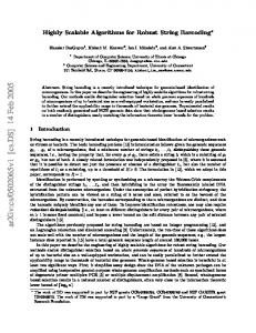
Acoustic feedback is a phenomenon that occurs in sound reinforcement systems, e.g., public-address systems and hearing aids. Since this thesis focuses on hearing aids, in the following the general implications of acoustic feedback are discussed in the context of hearing aids if not mentioned otherwise. Specifically, we consider behindthe-ear (BTE) hearing aids, where one or more microphones are placed behind the ear of the hearing aid wearer, and in-ear hearing aids, where the microphones are placed in the ear of the hearing aid wearer. If only a single microphone is available that is used for acoustic feedback suppression, this constitutes a singleloudspeaker single-microphone (SLSM) system, while if multiple microphones are available and used for feedback suppression, this constitutes a single-loudspeaker multi-microphone (SLMM) system. Acoustic feedback is created when a sound is picked up by a microphone, played back through a loudspeaker, and again picked up by the same microphone after passing through the acoustic feedback path, essentially creating an electro-acoustical closed-loop. In general, the acoustic feedback path contain parts that belong to the hearing aid loudspeaker and microphone as well as the acoustic path between these transducers, including, e.g., the ear canal. Figure 1.1 depicts exemplary amplitude responses of acoustic feedback paths measured in free field and with a telephone receiver in close distance. As can be observed, both acoustic feedback paths have their largest peak around 4 kHz and only little energy is present in frequencies below 1.5 kHz and above 7 kHz. Additionally, a telephone receiver (or other objects) close to the ear can alter the amplitude response significantly. Furthermore, these changes occur quickly when a person uses the telephone. On the contrary, when the hearing aid position is altered slightly or a person is chewing [10] smaller variations are observed that generally occur slowly over time. The acoustic feedback typically becomes a problem when the amplification of the loudspeaker is larger than the dampening of the acoustic propagation between the loudspeaker and the microphone. From Figure 1.1 the maximum stable gain (MSG) of the hearing corresponds to a value of approximately 15 dB for the free field condition. If additional processing is used to suppress the acoustic feedback, the resulting increase in the MSG is called the added stable gain (ASG). When the acoustic feedback occurs, the perceived quality of the signal is degraded and annoying audible artifacts are often perceived as reverberating echoes, howling or whistling. Consider the SLSM acoustic scenario depicted in Figure 1.2, where the microphone signal y[k] at discrete time k consists of the incoming signal x[k] and the feedback component f [k], i.e., y[k] = x[k] + f [k].
(1.1)
1.1 acoustic feedback and hearing aids
0
Free field Telephone close
Magnitude / dB
-10 -20 -30 -40 -50 -60 1000
2000
3000
4000
5000
6000
7000
8000
f / Hz
Figure 1.1: Exemplary amplitude responses of two different acoustic feedback paths of a behind-the-ear hearing aid measured in free-field and with a telephone receiver in close distance.
u[k]
G(q, k)
H(q, k)
f [k]
y[k]
x[k]
Figure 1.2: Generic single-loudspeaker single-microphone closed-loop system.
3
4
introduction
The microphone signal is processed by the hearing aid forward path G(q, k), where q denotes the discrete-time delay operator, forming the loudspeaker signal u[k], i.e., u[k] = G(q, k)y[k].
(1.2)
The loudspeaker signal is then fed back via the acoustic feedback path H(q, k) between the loudspeaker and the microphone, resulting in the feedback component f [k] as f [k] = H(q, k)u[k].
(1.3)
Using (1.1) and (1.3) in (1.2), the closed-loop transfer function C CL (q, k) relates the loudspeaker signal to the incoming signal and is given by C CL (q, k) =
1 u[k] = , CL x[k] 1 − O (q, k)
(1.4)
where OCL (q, k) denotes the open-loop transfer function, i.e., OCL (q, k) = G(q, k)H(q, k).
(1.5)
Assuming time-invariance of the acoustic feedback path and the hearing aid forward path, the Nyquist stability criterion1 [13] states that the closed-loop system is unstable if and only if for any frequency the following two conditions are fulfilled 1. Amplitude condition: the magnitude of the open-loop transfer function is equal or larger than one. 2. Phase condition: the phase response at this frequency is a multiple of 2π, i.e., the signal adds up constructively after passing the closed-loop. Note that even if both conditions are not fulfilled, the perceptual quality of the loudspeaker signal may be reduced, e.g., when the magnitude of the open-loop transfer function is larger than one and its phase is not exactly a multiple of 2π.
1.2
Overview of Feedback Suppression Methods
In this section we provide an overview of different feedback suppression methods, which can be broadly classified into the following three classes [11, 14]: 1. Feedforward algorithms that aim at mitigating the amplitude or phase condition of the Nyquist criterion by using non-linearities in the forward path. 2. Feedback algorithms that aim at obtaining an estimate fˆ[k] of the feedback component and subtracting this estimate from the microphone signal. These algorithms will be briefly reviewed in Section 1.4 and more specifically addressed in Chapter 3. 1 As mentioned in [11] for a time-varying system the so-called circle criterion should actually be used to define stability [12, Ch. 5]. However, the Nyquist criterion is commonly used in the feedback cancellation literature assuming a slowly varying system.
1.3 feedforward feedback suppression
3. Spatial filtering algorithms that rely on the availability of multiple microphones and aim at designing a spatial filter. This spatial filter aims at canceling the feedback contribution of the loudspeaker in the microphone signals by steering a spatial null into the location of the loudspeaker (cf. Section 1.5). While feedforward algorithms, which modify the loudspeaker signal, usually provide a trade-off between a limited feedback suppression performance and perceptually audible distortions, feedback algorithms, which aim at estimating the feedback component in the hearing aid microphone, theoretically allow for perfect feedback suppression performance. At the same time they avoid the introduction of audible distortions. Similarly, spatial filtering algorithms exploiting multiple microphones theoretically allow for perfect feedback suppression and can be designed in such a way that they avoid the introduction of audible distortions. While usually these approaches for feedback suppression are treated independently, a combination of at least two of these approaches is used in a practical application, e.g., [15–19]. Although this thesis considers the hearing aid application, several approaches for feedback suppression have been mainly investigated in the context of public address systems, e.g., feedforward algorithms. However, since the general scenario is very similar, in the remainder of this section we will only make a clear distinction between the hearing aid application and public address systems when necessary.
1.3
Feedforward Feedback Suppression
Feedforward feedback suppression algorithms generally use non-linearities in the hearing aid forward path to reduce the impact of acoustic feedback (cf. Figure 1.3). These include gain reduction methods that aim at mitigating the amplitude condition of the Nyquist criterion (cf. Section 1.3.1) and phase modulation methods that aim at mitigating the phase condition of the Nyquist criterion (cf. Section 1.3.2).
1.3.1 Gain Reduction Gain reduction methods aim at mitigating the amplitude condition of the Nyquist criterion. Accordingly, the gain in the forward path is reduced when instability of the system is detected. In general, these methods consist of a detection stage and a gain reduction stage and are usually inherently reactive, i.e., they require instability or howling to occur before reducing the gain. Only few methods act in a proactive fashion, i.e., they aim at applying a gain reduction before instability or howling occurs. Gain reduction methods can be categorized depending on the bandwidth and whether the detection and gain reduction are performed separately or jointly. Depending on the bandwidth different methods can be applied, e.g., broadband gain reduction, e.g., [20], subband gain reduction, e.g., [21] and notch-filter based gain reduction, e.g., [22–28]. On the one hand, broadband gain reduction and subband
5
6
introduction u[k] NL
G(q, k)
H(q, k)
f [k]
y[k]
x[k]
Figure 1.3: Generic SLSM closed-loop system with a non-linearity in the forward path.
gain reduction are usually two-stage approaches that comprise a separate howling or instability detection and verification stage and a separate bandwidth-dependent gain reduction stage. On the other hand, notch-filter based gain reduction can be performed using a two-stage approach or using a one-stage approach where howling detection and gain reduction is performed jointly. To detect and verify candidate howling components, different howling criteria have been proposed in the literature that include spectral as well as temporal criteria [11, 29]. Usually, the candidate howling components have similar properties as tonal components, e.g., a sustained violin note can be easily confused with a howling component. Therefore, on the one hand, the spectral criteria aim at detecting and discriminating the howling component from a tonal component by means of the entire spectrum, their (sub)harmonics or using the neighboring frequencies around a candidate howling component. On the other hand, temporal features aim at detecting and discriminating the howling component by means of its longer sustain and its exponentially increasing energy compared to a tonal component [20, 30, 31]. Furthermore, spectro-temporal criteria [32] or the combination of spectral and temporal features [29, 33] have been proposed to allow for an improved detection of howling components. Once one or more howling components have been detected, the broadband or subband gain is reduced or one or multiple notch-filters are used to remove these howling components. Here it should be noted that a broadband gain reduction can reduce the howling but obviously does not increase the MSG of the hearing aid. In contrast, based on results from the statistical properties of acoustic feedback path [34] the MSG of the hearing aid may be increased by up to approximately 10 dB [11] when using subband gain reduction or notch-filter based gain reduction. However, this increase in the MSG comes at the cost of a distorted loudspeaker signal, i.e., due to the attenuation of spectral components the loudspeaker signal is modified with undesired spectral changes. Note that these numbers are estimates based on the
1.3 feedforward feedback suppression
statistics of acoustic feedback paths and frequently for real automated systems no specific improvements are reported [11]. Nevertheless, it has been reported in [35, 36] when the tuning of multiple notch-filters is carried out manually for a time-invariant public address system the MSG may be increased by up to 15–20 dB. While broadband and subband gain reduction can be easily implemented when the forward path gain function uses subband processing (which is commonly the case), notch-filters usually are a separate processing stage and hence act independently of the forward path gain function. Different design procedures exist to design notch-filters with different bandwidths and center frequencies. For the one-stage notch-filter based gain reduction usually adaptive notch-filters are used. Due to their easy and stable implementation, the first proposed approaches using adaptive notch filters for feedback cancellation were using finite impulse response (FIR) filters [22, 26, 37]. In order to reduce the large filter order usually required in the FIR filter based adaptive notch filter, later approaches used infinite impulse response (IIR) filters [23, 27, 28, 38]. These IIR filters can be implemented using a so-called biquadratic filter structure [39–43], i.e., a second-order filter, and thus require only a short delay and lower computational cost compared to FIR filters. While biquadratic filters can be designed a priori, adaptive IIR filter based notch filtering aims at adaptively minimizing a least-squares cost function. However, for the problem at hand this cost function is non-convex such that its global optimum may not be obtained. Nevertheless, different approaches have been presented that aim either at obtaining a solution by trying to circumvent the non-convexity or at obtaining a solution close to the global optimum, e.g., [23, 27, 28]. For the two-stage notch filter based gain reduction, similarly to the broadband and subband gain reduction methods, the candidate howling component is first identified and verified. Subsequently, one or multiple biquadratic IIR filter based notch filters with appropriate bandwidths and center frequencies are used. Recently, a pro-active notch-filter based gain reduction has been proposed [16, 44], where an adaptive estimate of the acoustic feedback path (cf. Section 1.4) is used to estimate the most critical frequencies, i.e., those that are expected to lead to howling, and reduce the gain at those frequencies. While usually gain reduction methods are applied in an SLSM scenario, in [45] it has been proposed to apply a binaural coherence-based scheme to the problem of feedback cancellation in hearing aids, i.e., using an SLMM scenario. This method can be considered a one-stage subband gain reduction stage, where based on the coherence between both hearing aids a real-valued gain is applied to the microphone signals. This is motivated by the observation that acoustic feedback usually does not occur in both hearing aids simultaneously at the same frequency. 1.3.2 Phase-Modulation In contrast to gain reduction methods, phase-modulation methods generally aim at mitigating the phase condition of the Nyquist criterion in order to increase the stability of the system. The general class of phase-modulation methods includes methods
7
8
introduction
that perform [46, 47]: frequency shifting, e.g., [34, 48–55], true phase-modulation, e.g., [47, 56], amplitude modulation, frequency modulation, e.g., [57] and delay-modulation [37, 47]. Frequency shifting aims at smoothing the open-loop transfer function such that ideally the MSG depends only on the averaged transfer function instead of its maximum amplitude [34, 49, 51]. Thus, although belonging to the phase-modulation methods, frequency shifting effectively aims at mitigating the amplitude condition of the Nyquist criterion. Early implementations of the frequency shifting were based on analog single-sideband modulation [50, 52] or used the analog Hilbert transform [48, 53–55], while later implementations used the digital Hilbert transform [58, 59]. In [48, 60] it has been reported that by using frequency shifting the MSG can be increased by up to approximately 10–12 dB, depending on the properties of the acoustic feedback path. However, this comes at the expense of notable distortions, mostly perceived as beating. When limiting the gain to 6 dB below the MSG these distortions are claimed to become inaudible [49, 51]. Furthermore, the amount of frequency shifting influences the perceived quality of the signal, where several studies claim that a shift of approximately 5 Hz [34, 48, 49, 51] or even 10 Hz [18, 19, 61] provides a reasonable trade-off between performance and the amount of audible distortions. However, in [46] it has been shown that coloration artifacts are already noticeable for frequency shifts of as small as 2.3–4.2 Hz. Note that frequency shifting does not preserve the harmonic structure of the signal, which is especially audible for music signals. However, in [62] is has been shown that when bandwidth compression is used instead of frequency shifting, the harmonic relation can be preserved and the MSG can be increased by up to 10 dB. In phase-modulation methods the phase of the loudspeaker signal is modulated either in the broadband [47, 56, 63, 64] or in subbands [18, 65, 66]. Different approaches have been proposed using time-varying all-pass filters [63, 64], using singlesideband modulation based on a Hilbert transform [18, 47, 65], using sinusoidal phase modulation [56] or using frequency modulation [57], which can be considered a special case of phase modulation [11]. MSG improvements have been reported in the range from 4 dB [47, 56] to up to 7–8 dB [57, 67]. However, the perceptual quality of the signal is dependent on the modulation frequency and the modulation index, i.e., the magnitude of the modulation [46]. Therefore, in [18] an acoustic feedback suppression approach has been proposed that is based on a perceptually optimized phase modulation function [65] that depends on the ability of the human auditory system to detect phase modulations.
1.4
Adaptive Feedback Cancellation
In adaptive feedback cancellation (AFC) an adaptive filtering algorithm is used to obtain an estimate of the acoustic feedback path between the loudspeaker and the microphone [11, 15, 37] (cf. Figure 1.4). This estimate of the acoustic feedback path is used to compute an estimate of the feedback component in the microphone which is subsequently subtracted from the microphone signal. Note that since usu-
1.4 adaptive feedback cancellation u[k]
ˆ H(q, k)
G(q, k)
H(q, k)
f [k] e[k]
− +
y[k]
x[k]
Figure 1.4: Generic SLSM closed-loop system with an adaptive feedback canceller.
ally linearity of the acoustic feedback path is assumed, non-linear behavior of the loudspeaker and the microphone may influence the performance of the adaptive filtering algorithm [68]. In Section 1.4.1 an overview of different adaptive filter algorithms is given and different ways to improve the performance of AFC algorithms are outlined. In Section 1.4.2 the bias problem of the filter adaptation is briefly outlined and state-of-the-art solutions to reduce the bias are reviewed. 1.4.1 Adaptive Filtering Algorithms Commonly, the adaptation is performed in the time-domain [37, 69, 70]. In order to improve the AFC performance, several approaches have been proposed that use adaptation either in the subband-domain, e.g., [71–74], in the frequency-domain, e.g., [14, 74–78] or in some transform-domain, e.g., [79–81]. The performance of the adaptive filter is influenced by several parameters, including the step-size to update the adaptive filter coefficients, the auto-correlation properties of the filter input signal as well as the number of adaptive filter coefficients [82, 83]. Therefore, not only the choice of the adaptive filtering algorithm itself [84–86], but, in particular, the choice of the number of adaptive filter coefficients and the step-size is a nontrivial task. In general, a large number of filter coefficients allows to accurately estimate the acoustic feedback path at the expense of a reduced convergence speed and tracking capability. Similarly, the choice of a small step-size allows to accurately estimate slowly varying acoustic feedback paths at the expense of a reduced convergence speed and tracking capability for faster changes, while a large step-size allows for an increased convergence speed and tracking capability at the expense of a reduced accuracy for slowly varying acoustic feedback paths.
9
10
introduction
In order to reduce the number of filter coefficients and hence reduce the computational complexity and improve the convergence speed of the AFC algorithm, in [87, 88] it has been proposed to decompose the acoustic feedback path into a slowly time-varying part that could be estimated using a fixed filter and a rapidly timevarying part that could be estimated using an adaptive filter. The fixed filter would account for, e.g., transducer characteristics, microphone characteristics as well as individual ear characteristics, while the rapidly time-varying filter allows to track larger changes, e.g., in the presence of a telephone. In [89] the fixed filter was assumed to be a simple high-pass filter corresponding to the general high-pass characteristic observed in acoustic feedback paths in hearing aids. In a more sophisticated way, in [90] the fixed filter was estimated from multiple measurements of the acoustic feedback path, hence corresponding to parts that are common across a variety of acoustic feedback paths. Previously all-zero [90] and all-pole filters [91] have been used to model the fixed filter. In order to reduce the number of filter coefficients, one goal of this thesis is to extend these approaches to the general pole-zero filter and develop novel optimization procedures to estimate a fixed common pole-zero filter from multiple measured acoustic feedback paths. Different approaches have been proposed to automatically select the step-size of the adaptive filter [19, 92–100]. However, due to the closed-loop system encountered in feedback cancellation, the automatic step-size selection is often challenging [93, 98]. One goal of this thesis is to develop algorithms that provide an automatic selection of the step-size. 1.4.2 Bias and Bias Reduction In theory, AFC allows for a perfect cancellation of the acoustic feedback. However, due to the closed-loop system, the estimate of the acoustic feedback is typically biased [101–105]. Hence, independent of the used adaptive filtering algorithm, the adaptive filter will converge to a biased solution. This bias can be reduced by decorrelating the incoming signal and the loudspeaker signal in the filter adaptation. Furthermore, note that the bias of the acoustic feedback path estimate is small if the gain of the hearing aid is large [106, 107]. However, when the gain is large instability and howling might occur more frequently for fast changing acoustic feedback paths. In order to completely mitigate the bias problem, first attempts have tried using a fixed feedback cancellation filter [10, 108, 109], however, at the expense of a reduced performance for time-varying acoustic feedback paths. Several approaches have been presented in the literature to reduce the impact of the bias or to reduce the bias itself when adaptively estimating the acoustic feedback path. This includes constrained adaptation of the adaptive filter [110], band-limited adaptation [111, 112], probe-noise injection [105, 113–116], using non-linearites and gain reduction in the forward path [18, 61, 64, 117–120], using the prediction-errormethod (PEM) [78, 89, 104, 121–123] or using an auxiliary microphone [124, 125]. In the following we briefly review these state-of-the-art approaches for AFC.
1.4 adaptive feedback cancellation
1. In order to reduce the bias, in [110] it has been proposed to constrain the adaptive filter to only deviate in a predefined margin from an initially obtained unbiased estimate. While this leads to a good estimate when the true acoustic feedback path does not deviate largely from the initial unbiased estimate, the adaptive filter may not be able to model large changes in the acoustic feedback path [126, 127]. Furthermore, when using a constrained adaptation the general solution will still remain biased to some extent. In [111, 112] it has been proposed to constrain the adaptation of the adaptive filter to a specific frequency region by using a band-limited adaptation. Since acoustic feedback typically only occurs in the frequency range above approximately 1.5 kHz, the adaptation is only carried out in this region where acoustic feedback is expected to occur. 2. Using probe-noise injection a probe noise is additionally injected to the loudspeaker signal, where the probe-noise is designed to be uncorrelated with the incoming signal [105, 113–116]. While probe-noise injection allows to improve the feedback cancellation performance and in fact may lead to an unbiased estimation [105], the design of the probe-noise is challenging since, on the one hand, it should be inaudible to avoid perceptual signal distortions while, on the other hand, its power should be maximized. Moreover, in [115] it has been shown that the convergence properties of the adaptive filter are reduced when using a probe-noise at the input of the adaptive filter. To enhance the identification based on the probe-noise in [128, 129] it has been proposed to use a long-term prediction filter, while in [130] it has been proposed to use reshaping filter to improve the convergence properties when using a shaped probe-noise. In [131, 132] it has been proposed to replace the high-frequency components of the incoming signal by a vocoded signal that is perceptually similar to the original incoming signal components, while in [96, 116] the use of two adaptive filters using either a probe-noise or the loudspeaker signal was proposed to increase the performance. In [133] a two-stage approach has been presented that uses two adaptive filters, where the first filter aims at identifying the impulse response of the complete closed-loop system, while the second filter operates on the output of the first filter and aims at identifying the acoustic feedback path. 3. Non-linear functions can be introduced in the hearing aid forward path that allow to reduce the bias in the adaptive filter adaptation [61], e.g., using phase modulation [18], frequency shifting [18, 120], frequency compression [117], half-wave rectification [61] or time-varying all-pass filters [64, 118, 119]. Theoretical analyses for stereophonic echo cancellation have shown that, when appropriately tuned, both frequency shifting [134] and phase modulation [66] or their combination [135] can perfectly decorrelate the loudspeaker signals. Hence, when applied in combination with an adaptive filter (see Section 1.4.1), these methods should theoretically allow for an improved identification of the acoustic feedback path. Other approaches combine AFC and gain reduction methods using either adaptive notch-filtering [25] or psycho-acoustic criteria for gain reduction in subbands [17, 136, 137]. However, similarly as for probe-
11
12
introduction
noise approaches, these non-linear functions and gain reduction methods need to be tuned and provide a trade-off between decorrelation and audible signal distortions. 4. In the prediction-error-method (PEM) it is assumed that the incoming signal can be modeled as an auto-regressive process, e.g., a white noise sequence that is shaped using a stable all-pole filter. The inverse of this all-pole filter can then be used to prewhiten the microphone signal and the loudspeaker signal prior to the adaptation [78, 89, 104, 121–123]. It can be shown that if the all-pole filter is exactly known and the white noise sequence can be recovered, an unbiased estimate of the acoustic feedback path may be obtained [104]. It should be noted that this model of the incoming signal provides a good approximation for unvoiced speech, while for voiced speech and especially music it only provides a rough approximation. Thus, in practice the bias cannot be removed completely but only its impact on the filter adaptation may be reduced. Different variants of the PEM have been proposed using a fixed prewhitening filter [89] and using an adaptive prewhitening filter [78, 104]. Various adaptive filtering algorithms have been investigated in combination with an adaptive prewhitening filter including different time-domain algorithms [95, 104, 138– 148], frequency-domain algorithms [14, 16, 78, 149, 150], subband-domain algorithms [16, 19, 98, 100, 123] as well as other transform-domain algorithms [79]. Furthermore, simplified prewhitening filter updates [151] as well as more advanced models for the incoming signal have been proposed [152] that also account for harmonic excitation signals [153–156]. Additionally, the combination with proactive notch-filters [16, 44], probe-noise injection [157] and noise vocoding [131], single-microphone noise reduction [158, 159] and an inverse gain filter [142] have been proposed. Theoretical analyses of AFC based on prewhitening have been performed in [160–163], showing that the prewhitening approach converges to a stationary point for sinusoidal signals [160], has a reduced performance in case of imperfect modelling of the incoming signal [161], but is not influenced by the incoming signal leaking into the ear canal [163]. 5. To reduce the impact of the incoming signal on the adaptive filter adaptation used to cancel the acoustic feedback in a primary microphone, an auxiliary microphone that contains less acoustic feedback can be employed [124, 125]. In contrast to the previously mentioned approaches that consider a SLSM system, this approach can only be applied in SLMM systems. While this approach heavily relies on a good positioning of the main microphone and the auxiliary microphone, it theoretically allows to reduce the bias such that the performance in terms of feedback cancellation in the main microphone is similar to the performance if only the auxiliary microphone was used. In contrast to prewhitening using, e.g., the PEM, the bias does not rely on the correlation properties of the incoming signal but relies on the positioning of the auxiliary microphone. Extensions of this approach have been proposed using different adaptive filtering algorithms [80, 164–166] and a combination with a prewhitening filter to further reduce the bias [167]. In [168] a similar approach
1.5 spatial filtering based feedback suppression u[k]
G(q, k)
H(q, k) f1 [k] . . . fM [k] e˜[k] W(q)
y1 [k] .. .
x1 [k] .. .
yM [k]
xM [k]
Figure 1.5: Generic SLMM closed-loop system with a fixed beamformer.
was applied to binaural hearing aids, where the signal from the hearing aid on the other ear was used to improve the feedback cancellation performance.
1.5
Spatial Filtering based Feedback Suppression
Spatial filtering methods exploit the availability of multiple microphones to steer a spatial null towards the position of the loudspeaker (cf. Figure 1.5). Similarly, multiple loudspeakers can be used to steer a spatial null towards the position of a microphone [169]. Since in a hearing aid usually only a single loudspeaker is available, multi-microphone spatial filtering has been mainly investigated. While spatial filtering provides the capability of perfectly suppressing the acoustic feedback, its practical applicability in BTE has been limited due to the time-varying nature of the acoustic feedback paths [126, 170] and these approaches have been mainly investigated in combination with noise reduction algorithms [171, 172]. However, for a custom multi-microphone earpiece [173] with two microphones in the vent and a third microphone located in the concha, this approach may prove beneficial since the acoustic feedback paths may be assumed to be rather time-invariant. Therefore, one goal of this thesis is to develop different null-steering beamformer design procedures exploiting multiple microphones for feedback suppression which can be combined with AFC algorithms to cancel the residual feedback component in the beamformer output.
13
14
introduction
1.6
Thesis Outline and Main Contributions
The main objective of this thesis is to develop improved algorithms for acoustic feedback suppression in hearing aids. The main focus is to enhance the performance of adaptive filtering algorithms by reducing the number of the required filter coefficients and improving the trade-off between fast convergence and a good steady-state performance and to develop fixed spatial filter design methods that can be applied in a custom multi-microphone earpiece. The main contributions of this thesis are threefold. First, we propose several optimization procedures that allow to compute a fixed common pole-zero filter from multiple measured acoustic feedback paths, allowing to reduce the number of adaptive filter coefficients. Second, we propose to use an affine combination of two adaptive filters with different step-sizes to overcome the limitations associated with a single fixed step-size. Third, we propose several optimization procedures to design a fixed null-steering beamformer that can be used for acoustic feedback suppression and can be combined with an adaptive filter to cancel the residual feedback component. In the remainder of this section we give a chapter-by-chapter overview of this thesis, summarize the main findings, and provide a list of publications that have been produced in the context of this thesis. Figure 1.6 depicts a schematic overview of this thesis. In Chapter 2 we formally introduce the mathematical notation used in this thesis and present the signal processing framework for acoustic feedback cancellation for the single-loudspeaker single-microphone (SLSM) as well as for the singleloudspeaker multi-microphone (SLMM) system. We derive stability conditions for each of these systems and present instrumental performance measures that are used throughout this thesis to assess the benefit of the proposed algorithms. In Chapter 3 we present a detailed treatment of existing AFC algorithms. We specifically focus on the SLSM scenario and introduce the normalized least mean squares (NLMS) in the time-domain as an adaptive filtering algorithm to identify the acoustic feedback path. Furthermore, we show how the correlation between the loudspeaker signal and the incoming signal leads to a biased solution when estimating the acoustic feedback path. Moreover, we present two different algorithms to reduce this bias in the filter adaptation, i.e., subband adaptive filtering and the PEM, for which we present time-domain and frequency-domain implementations. In Chapter 4 we propose several optimization procedures to compute a common pole-zero filter from multiple acoustic feedback paths. We first derive different leastsquares optimization procedures minimizing the misalignment and subsequently derive different min-max optimization procedures that aim at directly maximizing the MSG. Since the resulting cost functions are non-linear in the parameters, we propose to use an iterative optimization procedure. In order to guarantee the stability of the common pole-zero filter, we propose to incorporate either a constraint based on the positive realness of the frequency response of the all-pole component of
1.6 thesis outline and main contributions
Chapter 2 acoustic setup and performance measures
Chapter 3 adaptive feedback cancellation
Chapter 4 common part optimization for afc in hearing aids
Chapter 5 affine combination of adaptive filters for afc
Chapter 6 feedback cancellation based on null-steering
Chapter 7 conclusion & outlook
Appendix B measurement of acoustic feedback paths Figure 1.6: Schematic overview of this thesis.
15
16
introduction
the common filter or a constraint based on Lyapunov theory. While the constraint based on the positive realness leads to a linear programming (LP) problem or a quadratic programming (QP) problem, the constraint based on Lyapunov theory leads to a semidefinite programming (SDP) problem. We experimentally show that using the proposed common pole-zero filter is favorable compared to using either the existing common all-zero filter or common all-pole filter and demonstrate the MSG improvements that can be obtained by the proposed optimization procedures. Furthermore, we experimentally validate that, when integrated with the state-ofthe-art PEM AFC algorithm, the proposed common pole-zero filter can be used to reduce the number of adaptive filter coefficients and improve the convergence speed. Publications associated with this chapter are [174–178]. In Chapter 5 we propose an AFC algorithm based on an affine combination of two adaptive filters. For correlated loudspeaker and incoming signals we show that not only the adaptive filters themselves lead to a biased solution but also the optimal combination parameter is biased. We show that integrating the PEM leads to an unbiased optimal combination parameter under certain conditions. Finally, we propose to perform the affine combination for the partitioned block frequency-domain adaptive filter (PBFDAF) with a frequency-dependent combination parameter. Experimental results indicate that using the proposed PBFDAF-based affine combination leads to an improved performance compared to using a single PBFDAF filter. A publication associated with this chapter is [179]. In Chapter 6 we propose to use a null-steering beamformer to cancel the acoustic feedback contribution in the microphone(s) of a custom multi-microphone in-ear earpiece. We present different design methods that aim at obtaining the (robust) beamformer coefficients. To obtain the null-steering beamformer coefficients, we first propose different least-squares optimization procedures minimizing the residual feedback power. Second, we propose different min-max optimization procedures that aim at directly maximizing the MSG for the considered SLMM scenario. In order to preserve the incoming signal, we consider two different constraints. In the first constraint we set the beamformer coefficients in the reference microphone to a delay, which, however, does not directly control for distortions of the incoming signal. In the second constraint we propose to directly control the distortions by using a constraint based on the relative transfer function (RTF) of the incoming signal. Experimental results using measured acoustic feedback paths from a custom multimicrophone earpiece show that using the proposed optimization procedures a robust average ASG of more than 50 dB can be achieved without significantly reducing the quality of the incoming signal. Furthermore, combining with an AFC algorithm using the PEM the performance can be further increased, where results indicated that the performance of the AFC algorithm and the fixed null-steering beamformer are complementary. Publications associated with this chapter are [180–183] In Chapter 7 the main findings of this thesis are summarized and suggestions for further research are given.
2 ACOUSTIC SETUP AND PERFORMANCE MEASURES
In this chapter the general notation, the considered hearing aid setups as well as the instrumental performance measures used in the remainder of this thesis are presented. In Section 2.1 the considered SLSM system and SLMM system and the resulting closed-loop systems are discussed. Based on these descriptions, in Section 2.2 several instrumental performance measures are introduced to evaluate the feedback cancellation performance.
2.1
Acoustic Systems and Notation
2.1.1 Notation, Transfer Functions and Frequency Response In this thesis generally we denote scalars as x, vectors using x and matrices using X. Furthermore, for convenience we adopt the notation proposed in [184] and use q −1 to denote the discrete delay operator. The acoustic transfer function (ATF) H(q, k) is defined as H(q, k) =
LX H −1
hi [k]q −i ,
i=0 T
= h [k]q,
(2.1) (2.2)
where [·]T denotes transpose operation, h[k] is the LH -dimensional coefficient vector of H(q, k) and q the vector of integer delays of appropriate size, i.e., h iT h[k] = h0 [k] h1 [k] . . . hLH −1 [k] , h iT q = 1 q −1 . . . q −LH +1 .
(2.3) (2.4)
17
18
acoustic setup and performance measures
Using this notation the output y[k] of a filtering operation of a signal x[k] with the ATF H(q, k) can be written as (2.5)
y[k] = H(q, k)x[k] = hT [k]x[k], where x[k] is the LH -dimensional vector of delayed elements of x[k], i.e., h x[k] = x[k] x[k − 1] . . .
x[k − LH + 1]
iT
.
(2.6)
Furthermore, the frequency response at discrete frequency ωn using an NF F T -point discrete Fourier transform (DFT) is defined as H(ωn , k) =
LX H −1
hi [k]e
−j N2πni
FFT
(2.7)
,
i=0 T
(2.8)
= f (ωn )h[k],
where f(ωn ) is the LH -dimensional vector of the NF F T -point DFT coefficients, i.e., h f(ωn ) = 1
e
−j N2πn
FFT
...
e
−j
2πn(LH −1) NF F T
iT
.
(2.9)
Furthermore, we define the NF F T × NF F T -dimensional DFT matrix 1 1 1 ... 1 2π(NF F T −1) −j 2π −j 4π −j 1 NF F T e NF F T e NF F T ... e 4π(NF F T −1) .. −j −j N 4π −j N 8π . N FNF F T = FFT FFT FFT . e e e 1 . . .. .. .. .. . . . . . 4π(NF F T −1) 2π(NF F T −1)(NF F T −1) 2π(NF F T −1) −j −j −j NF F T NF F T NF F T 1 e e ... e (2.10) 2.1.2 Closed-Loop System without Feedback Suppression Consider the SLSM system depicted in Figure 1.2, where the microphone signal y[k] at discrete time k consists of the incoming signal x[k] and the feedback component f [k], i.e., y[k] = x[k] + f [k].
(2.11)
The microphone signal is processed by the forward path G(q, k), forming the loudspeaker signal u[k], i.e., u[k] = G(q, k)y[k],
(2.12)
2.1 acoustic systems and notation
where G(q, k) is of length LG . The loudspeaker signal is then fed back via the acoustic feedback path H(q, k) of length LH between the loudspeaker and the microphone. The resulting feedback component f [k] is computed as (2.13)
f [k] = H(q, k)u[k].
Using (2.11) and (2.13) in (2.12), the closed-loop transfer function C CL (q, k) without feedback suppression is defined as C CL (q, k) =
1 u[k] = , x[k] 1 − OCL (q, k)
(2.14)
where OCL (q, k) denotes the open-loop transfer function, i.e., OCL (q, k) = G(q, k)H(q, k).
(2.15)
Assuming time-invariance of the acoustic feedback path and the hearing aid forward path, i.e., H(q, k) = H(q) and G(q, k) = G(q), the Nyquist stability criterion1 [13] states that the closed-loop system is unstable if and only if for any discrete frequency ωn the following two conditions are fulfilled: 1) the magnitude of the open-loop transfer function is equal or larger than one and 2) the phase response at this frequency is a multiple of 2π, i.e., the signal adds up constructively after passing the closed-loop. Mathematically the time-invariant closed-loop system C CL (q, k) = C CL (q) is thus unstable if and only if the following two conditions of the time-invariant open-loop transfer function OCL (q, k) = OCL (q) are fulfilled simultaneously (
(2.16a)
|OCL (ωn )| ≥ 1, ∠O
CL
(ωn ) = r2π,
r = Z.
(2.16b)
Note that even if both conditions are not fulfilled, the perceptual quality of the loudspeaker signal may be reduced, e.g., when the magnitude of the open-loop transfer function is larger than one and its phase is not exactly a multiple of 2π. 2.1.3 Single-Loudspeaker Single-Microphone System ˆ k) of Consider the SLSM system depicted in Figure 2.1 where an estimate H(q, ˆ H(q, k) is used to compute an estimate f [k] of the feedback component f [k] in order to reduce the acoustic feedback in the microphone. This estimate can be obtained, e.g., using the AFC algorithms discussed in Section 1.4. The microphone signal y[k] is the sum of the incoming signal x[k] and the feedback component f [k], i.e., y[k] = x[k] + f [k].
(2.17)
1 Note that as metioned in [11] for a time-varying system in fact the so-called circle criterion should be used to define stability [12, Ch. 5], however, the Nyquist criterion is commonly used in the feedback cancellation literature assuming a slowly varying system.
19
20
acoustic setup and performance measures u[k]
ˆ H(q, k)
G(q, k)
H(q, k)
fˆ[k] e[k]
f [k]
− +
y[k]
x[k]
Figure 2.1: Generic single-loudspeaker single-microphone hearing aid system with feedback suppression.
An estimate fˆ[k] of the feedback component f [k] is subtracted from the microphone signal, resulting in the so-called error signal e[k], i.e., e[k] = y[k] − fˆ[k].
(2.18)
The loudspeaker signal u[k] is obtained by processing the error signal using the hearing aid forward path G(q, k), i.e., (2.19)
u[k] = G(q, k)e[k]. The feedback component in the microphone is defined as
(2.20)
f [k] = H(q, k)u[k],
where H(q, k) is the acoustic feedback path of length LH between the loudspeaker and the microphone. The estimated feedback component is defined as ˆ k)u[k], fˆ[k] = H(q,
(2.21)
ˆ k) is an (adaptive) filter estimate of length L ˆ of the acoustic feedback where H(q, H path H(q, k). Using (2.17), (2.18), (2.20), and (2.21) in (2.19), the loudspeaker signal can be rewritten as (2.22)
ˆ k)u[k]), u[k] = G(q, k)(y[k] − H(q, ˆ k)u[k]), = G(q, k)(x[k] + H(q, k)u[k] − H(q, ˆ k))u[k], = G(q, k)x[k] + G(q, k)(H(q, k) − H(q, =
G(q, k) ˆ k)) 1 − G(q, k)(H(q, k) − H(q, | {z } C(q,k)
x[k],
(2.23) (2.24) (2.25)
2.1 acoustic systems and notation u[k]
G(q, k)
ˆ H(q, k)
H(q, k) f1 [k] . . . fM [k]
e[k]
− +
e˜[k] W(q, k)
y1 [k] . . .
x1 [k] . . .
yM [k]
xM [k]
Figure 2.2: Generic single-loudspeaker multi-microphone hearing aid system with feedback suppression.
where C(q, k) denotes the closed-loop transfer function of the SLSM system in Figure 2.1, and the open-loop transfer function is defined as ˆ k)). O(q, k) = G(q, k)(H(q, k) − H(q,
(2.26)
Similarly as for OCL (q, k) in (2.15), the magnitude and phase conditions in (2.16) apply to O(q, k). Note that the system is stable independently of the forward path ˆ k) is able to perfectly estimate the acoustic feedback path, i.e., if the filter H(q, ˆ k) = H(q, k), such that the loudspeaker signal is given by H(q, u[k] = G(q, k)x[k].
(2.27)
Algorithms for the SLSM system will be presented in Chapters 3, 4, and 5 of this thesis. In Chapter 3 we present an overview on relevant adaptive filters for this thesis and in Chapter 4 and 5 we propose two different approaches to improve the performance of adaptive filtering algorithms for AFC. 2.1.4 Single-Loudspeaker Multi-Microphone System Consider the SLMM system depicted in Figure 2.2 with M microphones. Similarly as in (2.17), the mth microphone signal ym [k], m = 1, . . . , M , is the sum of the incoming signal xm [k] and the feedback component fm [k], i.e., ym [k] = xm [k] + fm [k].
(2.28)
21
22
acoustic setup and performance measures
To combine all microphone signals, a filter-and-sum beamformer, acting as a spatial pre-processor, is applied to the microphone signals resulting in the beamformer output signal e˜[k], i.e., e˜[k] =
M X
(2.29)
Wm (q, k)ym [k],
m=1
=
M X
Wm (q, k)xm [k] +
m=1
M X
Wm (q, k)fm [k],
(2.30)
m=1
|
{z
f˜[k]
}
where Wm (q, k) is the weighting function of the beamformer in the mth microphone. An estimate fˆ[k] of the residual feedback component f˜[k] is subtracted from the beamformer output signal, i.e., e[k] = e˜[k] − fˆ[k].
(2.31)
The loudspeaker signal is then obtained by processing the error signal using the hearing aid forward path G(q, k), i.e., u[k] = G(q, k)e[k].
(2.32)
Using the loudspeaker signal u[k], the feedback component fm [k] in the mth microphone is defined as fm [k] = Hm (q, k)u[k],
(2.33)
where Hm (q, k) is the mth acoustic feedback path of length LH between the loudspeaker and the mth microphone. The estimated residual feedback component is defined as ˆ k)u[k], fˆ[k] = H(q,
(2.34)
ˆ k) is an (adaptive) filter estimate of length L ˆ of the residual acoustic where H(q, H PM feedback path transfer function m=1 Wm (q, k)Hm (q, k). Using matrix and vector notation, equations (2.28), (2.31) and (2.33) can be written as y[k] = x[k] + f [k],
(2.35)
e˜[k] = W (q, k)y[k],
(2.36)
f [k] = H(q, k)u[k],
(2.37)
h iT y[k] = y1 [k] . . . yM [k] , h iT x[k] = x1 [k] . . . xM [k] , h iT f [k] = f1 [k] . . . fM [k] ,
(2.38)
T
where
(2.39) (2.40)
2.1 acoustic systems and notation
and h iT W(q, k) = W1 (q, k) . . . WM (q, k) , h iT H(q, k) = H1 (q, k) . . . HM (q, k) ,
(2.41) (2.42)
are the vectors of the beamformer weighting functions and the acoustic feedback path transfer functions, respectively. Using (2.31), (2.34), (2.35), (2.36), (2.37) and yT [k]W(q, k) = WT (q, k)y[k] in (2.32), the loudspeaker signal can be rewritten as (2.43) ˆ = G(q, k)((x [k] + H (q, k)u[k])W(q, k) − H(q, k)u[k]), (2.44) T T ˆ = G(q, k)x [k]W(q, k) + G(q, k)(H (q, k)W(q, k) − H(q, k))u[k], (2.45)
ˆ k)u[k]), u[k] = G(q, k)(yT [k]W(q, k) − H(q, T
= xT [k]
T
G(q, k)W(q, k)
, ˆ k)) 1 − G(q, k)(HT (q, k)W(q, k) − H(q, | {z }
(2.46)
C(q,k)
where C(q, k) denotes the closed-loop transfer function vector of the SLMM system in Figure 2.2. The corresponding open-loop transfer function is defined as ˆ k)). O(q, k) = G(q, k)(HT (q, k)W(q, k) − H(q,
(2.47)
Similarly as for OCL (q, k) in (2.15), the magnitude and phase conditions in (2.16) apply to O(q, k). It should be noted that differently from the SLSM system, in the SLMM system the system is stable independently of the applied forward path G(q, k) if one of the following conditions is fulfilled: 1. The beamformer W(q, k) only partially cancels the contribution of the loudˆ k) is able to perfectly esspeaker in the microphones and the filter H(q, timate the residual feedback component in the beamformer output, i.e., ˆ k) = HT (q, k)W(q, k), such that H(q, ˆ k) = 0. HT (q, k)W(q, k) − H(q,
(2.48)
2. The beamformer W(q, k) is able to perfectly cancel the contribution of the ˆ k) is used, i.e., loudspeaker in the microphones and/or no filter estimate H(q, ˆ H(q, k) = 0, such that HT (q, k)W(q, k) = 0.
(2.49)
If either of these two conditions is fulfilled, the loudspeaker signal is given by u[k] = G(q, k)WT (q, k)x[k].
(2.50)
This implies that depending on the beamformer design, distortions may be introduced to the incoming signal. This is an important aspect which will be taken into
23
24
acoustic setup and performance measures
account when considering algorithms for the SLMM system in Chapter 6 of this thesis. Note that obviously for M = 1 and W1 (q, k) = 1, the SLMM system is equivalent to the SLSM system discussed in Section 2.1.3.
2.2
Instrumental Performance Measures
In order to evaluate the performance of feedback suppression algorithms in hearing aids, several instrumental measures have been proposed in the literature [185–191]. Most of these measures assume that no access to the internal hearing aid signals, e.g., the output of the adaptive filter estimating the feedback component, is available. However, during the development of feedback cancellation algorithms access to all signals is available, enabling the use of intrusive measures. Commonly, the performance of AFC algorithms is evaluated by considering the convergence state of the adaptive filter compared to the true acoustic feedback path. The typical measures used to quantify the performance of an adaptive filter in a closed-loop system are the normalized misalignment and the MSG [190]. Using the MSG, the ASG and the effective closed-loop gain (ECLG) [19], which depends on the hearing aid forward path G(q, k), can be computed. While the normalized misalignment aims at quantifying the performance of the adaptive filter compared to a reference, the MSG is related to the stability of the hearing aid. Similarly, the ASG is used to describe the additional gain that can be applied in the hearing aid forward path when feedback suppression is performed, while the ECLG described the gain margin that is still available until instability will occur depending on the hearing aid forward path. In the following sections we will describe these measures for the SLSM and SLMM systems considered in the thesis. Since the algorithms developed in this thesis may require the availability of multiple measurements of the acoustic feedback path, these instrumental measures will also depend on the measurement. 2.2.1 Normalized Misalignment The normalized misalignment aims at quantifying the performance of an adaptive filter estimate compared to a reference, e.g., the true acoustic feedback path. For the single-loudspeaker single-microphone (SLSM) system (cf. Figure 2.1) the normalized misalignment ξi [k] for the ith measured acoustic feedback path, i = 1, . . . , I, is defined as the normalized squared Euclidean distance between the true acoustic feedback path coefficient vector hi [k] and the estimated acoustic feedback ˆ i [k], i.e., path coefficient vector h ξi [k] =
ˆ i [k]k22 khi [k] − h . khi [k]k22
(2.51)
2.2 instrumental performance measures
The normalized misalignment is similarly defined in the frequency-domain as NF P F T −1
ξi [k] =
ˆ i (ωn , k)|2 |Hi (ωn , k) − H
n=0 NF P F T −1
(2.52)
. |Hi (ωn
, k)|2
n=0
For the single-loudspeaker multi-microphone (SLMM) system (cf. Figure 2.2) the normalized misalignment ξi [k] for the ith measured acoustic feedback paths, i = 1, . . . , I, is computed as the normalized squared Euclidean distance between the residual beamformer transfer function HTi (q, k)W(q, k) and the estimated residual ˆ i (q, k), i.e., beamformer transfer function H
ξi [k] =
� M
2 �
P
ˆ hm,i [k]Wm (q, k) − hi [k]
m=1
2
M P m=1
(2.53)
,
khm,i [k]k22
where hm,i [k] is the LH -dimensional coefficient vector of the mth acoustic feedback path Hm,i (q, k). The normalized misalignment is similarly defined in the frequencydomain as NF P F T −1
ξi [k] =
n=0
2 ˆ |HH i (ωn , k)W(ωn , k) − Hi (ωn , k)|
NF P F T −1 n=0
,
(2.54)
HH i (ωn , k)Hi (ωn , k)
where [·]H denotes complex conjugate transpose (Hermitian). 2.2.2 Maximum Stable Gain and Added Stable Gain For a closed-loop system the maximum stable gain (MSG) is defined as the maximum gain that can be applied in the forward path until the stability conditions in (2.16) are violated. In order to derive a simplified expression, it is usually assumed that the phase condition in (2.16b) is fulfilled for all frequencies (providing a worstcase assumption), such that only the amplitude condition in (2.16a) is considered. Assuming a broadband forward path gain function G(q, k) = |G|q −dG with dG ≥ 1 a delay the MSG is obtained by rearranging and solving |O(ωn , k)| = 1 for the broadband gain |G|, e.g., [88]. For the closed-loop system without feedback suppression the maximum stable gain for the ith acoustic feedback path is defined as MCL i [k] =
1 . maxωn |Hi (ωn , k)|2
(2.55)
25
26
acoustic setup and performance measures
For the single-loudspeaker single-microphone system the maximum stable gain for the ith measured acoustic feedback path is defined as Mi [k] =
1
(2.56)
ˆ i (ωn , k)|2 maxωn |Hi (ωn , k) − H
Similarly, for the single-loudspeaker multi-microphone system the maximum stable gain for the ith measured acoustic feedback paths is defined as Mi [k] =
1 maxωn
|HH i (ωn , k)W(ωn , k)
ˆ i (ωn , k)|2 −H
.
(2.57)
The ASG is defined as the MSG ratio between the condition where the feedback suppression algorithm is applied and the condition where no feedback suppression algorithms is applied, i.e., Ai [k] =
Mi [k] . MCL i [k]
(2.58)
In the logarithmic domain it is hence defined as 10 log10 Ai [k] = 10 log10 Mi [k] − 10 log10 MCL i [k].
(2.59)
2.2.3 Effective Closed-Loop Gain In order to take into the account the forward path function of the hearing aid, the effective closed-loop gain (ECLG) is a measure of the gain margin that is available in the closed-loop system [19]. The ECLG can be computed using the open-loop transfer function and for the closed-loop system without feedback suppression the effective closed-loop gain for the ith measured acoustic feedback path is defined as EiCL [k] = max |OiCL (ωn , k)| ωn
= max |G(ωn )Hi (ωn )|. ωn
(2.60) (2.61)
In view of the magnitude condition of the Nyquist stability criterion a value of Ei < 1 indicates a stable system. Using the definition of the open-loop transfer in (2.26) the effective closed-loop gain for the single-loudspeaker single-microphone system for the ith measured acoustic feedback path is defined as ˆ i (ωn , k))|. Ei [k] = max |G(ωn , k)(Hi (ωn , k) − H ωn
(2.62)
Using the definition of the open-loop transfer in (2.47) the effective closed-loop gain for the single-loudspeaker multi-microphone system for the ith measured acoustic feedback path is defined as ˆ Ei [k] = max |G(ωn , k)(HH i (ωn , k)W(ωn , k) − H(ωn , k))|. ωn
(2.63)
2.3 summary
2.2.4 Speech Quality Measures In order to evaluate the perceived quality of speech signals processed by acoustic feedback cancellation algorithms, we will use the perceptual evaluation of speech quality (PESQ) measure [192]. It has been shown in [107] that for a speech signal the PESQ measure provides a reasonable correlation between estimated quality and subjective evaluated quality for AFC algorithms. The PESQ measure compares a processed signal with an (unprocessed) reference signal, which in the context of feedback cancellation for SLSM system is usually the incoming signal x[k] and for SLMM system is usually the incoming signal xm0 [k] in a reference microphone m0 . First, the processed signal and the reference signal are time-aligned and subsequently compared using a perceptual model that accounts for perceptual aspects of the human auditory system. The output of PESQ is an objective listening quality MOS in the range from -0.5 to 4.5, where the values will typically be similar to subjective MOS scores in the range of 1 to 4.5 [192].
2.3
Summary
In this chapter we formally introduced both considered acoustic systems, i.e., the SLSM system with a single microphone and the SLMM system with multiple microphones, and we presented several instrumental measures to quantify the performance of acoustic feedback cancellation algorithms. These measures include the normalized misalignment, the maximum stable gain (MSG) and added stable gain (ASG), and the effective closed-loop gain (ECLG). Finally, we introduced the perceptual evaluation of speech quality (PESQ) measure that will be used to evaluate the perceptual quality of the processed speech signals.
27
3 ADAPTIVE FEEDBACK CANCELLATION
In this chapter we will present a detailed overview of existing adaptive feedback cancellation (AFC) algorithms relevant for this thesis. In Section 3.1 we first present the continuous adaptive filtering algorithm. Since it is well known that for AFC the optimal solution of the continuous adaptive filtering algorithm is typically biased, in Section 3.2 we analyze this bias for the case of correlated incoming signals. In Section 3.3 we then present different existing AFC algorithms aiming to reduce this bias. In Section 3.3.2 we particularly focus on the prediction-error-method (PEM) which is used in this thesis. For conciseness we only consider the SLSM system described in Section 2.1.3. However, it should be noted that the adaptive feedback cancellation algorithms discussed in this chapter can generally also be applied in the SLMM system described in Section 2.1.4 to cancel the residual feedback component in the beamformer output.
3.1
Adaptive Filtering
Consider the SLSM system with an adaptive filter as depicted in Figure 3.1. The ˆ k) is ˆ opt of the adaptive filter H(q, optimal LHˆ -dimensional filter coefficient vector h minimizing the squared error signal [82, 83], i.e., the following cost function ˆ = E{e2 [k]}, JW F (h[k]) ˆ T [k]Ruu [k]h[k] ˆ − 2h ˆ T [k]Ruu [k]y[k] + y 2 [k] =h
(3.1) (3.2)
where we used (2.17) and (2.21), E{·} denotes mathematical expectation and Ruu [k] = E{u[k]uT [k]} and ruy [k] = E{u[k]y[k]} denote the auto-correlation matrix and the cross-correlation vector, respectively, and u[k] is the LHˆ -dimensional vector of delayed elements of u[k] similarly defined as x[k] in (2.6). The optimal closed-form solution, i.e., the so-called Wiener filter, is given as ˆ opt [k] = R−1 h uu [k]ruy [k].
(3.3)
29
30
adaptive feedback cancellation u[k]
ˆ H(q, k)
G(q, k)
H(q, k)
f [k] e[k]
− +
y[k]
x[k]
Figure 3.1: Generic single-loudspeaker single-microphone hearing aid closed-loop system with an adaptive filter.
Note that the filter is obtained from expectations, i.e., ensemble averages, and thus is optimal in a stochastic sense. Note that obtaining these ensemble averages is not possible in practice and hence they are usually substituted by time averages. In practice the computation of the optimal solution at each time-step k is not possible since the the exact statistical information of the data is unknown and may even change over time. Therfore, usually adaptive algorithms are used to approximate the optimal solution as closely as possible. There are two main classes of adaptive algorithms [83]: 1) steepest-descent type of algorithms and 2) stochastic-gradient type of algorithms. While steepest-descent algorithms update an estimate of the acoustic feedback path using the negative gradient of the Wiener filter cost function in (3.1) with respect to the filter coefficient vector and still require the statistical information of the data to be available, stochastic-gradient type of algorithms substitute the statistical information using instantaneous approximations. In the following we first present how the Wiener filter estimate can be obtained using steepest-descent type algorithms and derive the corresponding stochastic-gradient type of algorithms that are used in practice. ˆ is given by The gradient of (3.1) with respect to h[k] ˆ ˆ ∇h[k] ˆ JW F (h[k]) = −2(ruy [k] − Ruu [k]h[k]), = −2E{u[k]e[k]}.
(3.4) (3.5)
ˆ is then given as [83] The adaptive update equation of the estimate h[k] ˆ + 1] = h[k] ˆ + µ[k]BE{u[k]e[k]}, h[k
(3.6)
3.1 adaptive filtering
with µ[k] a possibly time-varying step-size parameter and B a positive-definite matrix. On the one hand, choosing B = I leads to the well-known steepest descent algorithm, i.e., ˆ + 1] = h[k] ˆ + µ[k]E{u[k]e[k]}. h[k
(3.7)
On the other hand, choosing B = (αI + Ruu [k])−1 leads to the regularized Newton method, also known as the Levenberg-Marquardt method [83], i.e., ˆ + 1] = h[k] ˆ + µ[k](αI + Ruu [k])−1 E{u[k]e[k]}, h[k
(3.8)
with α a positive regularization parameter. In stochastic gradient algorithms, the expectation operator on u[k]e[k] is dropped and instantaneous estimates from the available data are used. The update equation for the stochastic-gradient algorithm that corresponds to the steepest-descent update in (3.7) is then given as ˆ + 1] = h[k] ˆ + µ[k]u[k] (y[k] − h ˆ T [k]u[k]) . h[k | {z }
(3.9)
e[k]
The most widely used algorithms in AFC are the least mean squares (LMS) and normalized least mean squares (NLMS) algorithm due to their stable adaptation and low computational complexity. The LMS algorithm is obtained from (3.9) by using a fixed step-size, i.e., µLM S [k] = µ,
(3.10)
while the NLMS algorithm is obtained from (3.9) by normalizing (3.10) with the (instantaneous) power of the input signal or is similarly obtained from (3.8) by using instantaneous approximations and applying the matrix inversion lemma [83], i.e., µN LM S [k] =
µ , uT [k]u[k] + α
(3.11)
with α a small positive regularization parameter to avoid division by zero. Note that while for the LMS algorithm a stable adaptation of the adaptive filter depends on the instantaneous power of the filter input u[k], for the NLMS algorithm a stable adaptation is guaranteed for values of 0 < µ < 2. However, it should be kept in mind that a stable adaptation of the adaptive filter does not guarantee stability of the closed-loop hearing aid system. Since the step-size µ controls the size of the update, a larger µ generally leads to a faster convergence at the expense of a larger steady-state misalignment of the adaptive filter [83]. Furthermore, on the one hand, using a longer filter length LHˆ generally leads a reduced convergence speed since more filter coefficients need to be updated but allows to model the unknown system H(q, k) more accurately. On the other hand, using a shorter filter length LHˆ leads to an increased convergence speed at the expense of less accurate modeling of the unknown system H(q, k) if LHˆ < LH , which is usually the case since LH is unknown in practice.
31
32
adaptive feedback cancellation
3.2
Bias Analysis
In this section we analyze the optimal solution in (3.3) and conclude that it is usually biased and only in certain conditions an unbiased estimate may be obtained [101, 102, 104, 105]. Assuming a sufficient order, i.e., knowledge of the length of the acoustic feedback path, i.e., LHˆ = LH , the optimal solution given in (3.3) can be rewritten in terms of the incoming signal x[k] and the acoustic feedback component f [k] using (2.17), i.e., −1 hopt [k] = R−1 uu [k]ruf [k] + Ruu [k]rux [k],
= =
−1 R−1 uu [k]Ruu [k]h[k] + Ruu [k]rux [k], h[k] + R−1 uu [k]rux [k],
(3.12) (3.13) (3.14)
where in the second step we made use of the definition of f [k] = uT [k]h[k] in (2.20). From (3.14) we observe that the optimal solution is unbiased if and only if the cross-correlation vector between the loudspeaker signal and the incoming signal rux [k] = 0. However, this is usually not the case as we will show in the following. Assuming that the forward path function is a broadband gain |G| and a delay dG ≥ 1, i.e., G(q, k) = |G|q −dG , and using (2.25), the cross-correlation vector rux [k] can be written as x[k − dG ] x[k − dG − 1] . (3.15) x[k] rux [k] = C(q, k)|G|E ... x[k − dG − LHˆ + 1] As can be observed from (3.15), if the delay dG is longer than the auto-correlation of the incoming signal x[k], an unbiased estimate may be obtained. E.g., if the incoming signal is white noise, then a delay of dG = 1 is sufficient to obtain an unbiased estimate. However, if the delay dG is chosen smaller than the auto-correlation of the incoming signal x[k], the solution will generally be biased. Note that the delay dG cannot be chosen arbitrarily large, as it determines the input-output delay of the hearing aid processing, which should be smaller than 10 ms [193]. However, typical sounds a hearing aid user is exposed to, e.g., speech and music, have longer autocorrelation times in the order of, e.g., 20 ms for speech signal and up to several seconds for sustained tones in music signals.
3.3
Bias Reduction Methods
As pointed out in Section 1.4 several methods exist to reduce the bias in the adaptive filter. These include subband adaptive filtering, constrained adaptation of the adaptive filter, probe-noise injection, non-linear processing of the loudspeaker signal, the PEM using prewhitening filters as well as using an auxiliary microphone. While probe-noise injection and non-linear processing of the loudspeaker signal alter the played back signal and may significantly reduce the quality of the speech
3.3 bias reduction methods
signal, using an auxiliary microphone relies on a good position of that microphone. In contrast, subband adaptive filtering, constrained adaptation and the PEM do not alter the loudspeaker signal and may hence provide a better quality. In this section we review different methods to reduce the bias in the adaptive filter adaptation that are used in the remainder of this thesis. These include the delayless subband adaptive filtering in Section 3.3.1 as well as the prediction-error-method (PEM) in Section 3.3.2. 3.3.1 Using Subband Adaptive Filters Subband adaptive filtering for AFC has been proposed in [71–74] to achieve a decorrelation of the incoming signal and the loudspeaker signal by applying the adaptive filtering in subbands. Different adaptive filterbank structures exist [194], e.g., an open-loop structure, which aims at minimizing the summation of the squared error across all subbands, and a closed-loop structure, which aims at minimizing the squared fullband error signal. In subband adaptive filtering a (decimating) analysis filterbank is used to split the loudspeaker signal and the incoming signal (when using an open-loop structure) or the error signal (when using a closed-loop structure) into subbands. Independent adaptive filters are then used in each subband and finally the fullband signal is reconstructed by applying a synthesis filterbank. Since applying an analysis and synthesis filterbank usually introduces a delay, a delayless subband architecture has been proposed in [195], where the fullband filter is reconstructed from the subband adaptive filters [196] and is applied on a sampleby-sample basis to the fullband signal. Such a delayless subband architecture was applied to AFC in, e.g., [18, 19], and will be used in this thesis in Chapter 6. More specifically, we consider a delayless filterbank using the closed-loop structure as proposed in [195]. The prototype filter used for the design of the analysis filterbank to split the signal into Ms subbands using a decimation factor of Ds = Ms /2 is a Kaiser-window [197], providing a good separation of the subbands [198]. In each of the subbands the adaptive filter of length Ls = LHˆ /Ds is updated using the NLMS update rule similarly as in (3.9) using (3.11). The corresponding fullband filter of length LHˆ is obtained by using the procedure described in [196]. 3.3.2 Prediction-Error-Method The prediction-error-method (PEM) aims at reducing the bias in the filter adaptation by using prewhitening filters to decorrelate the incoming signal x[k] and the loudspeaker signal u[k]. These prewhitening filters can be either fixed, e.g., assuming that the correlation properties of the incoming signal are known, or adaptive, aiming at estimating the correlation properties of the incoming signal. In the PEM it is generally assumed that the incoming signal can be adequately modeled as an auto-regressive model, which is reasonable, e.g., for speech signals. Figure 3.2 depicts the SLSM system where the PEM is used for AFC. The incoming signal is
33
34
adaptive feedback cancellation u[k]
ˆ k) A(q,
copy of ˆ H(q, k)
G(q, k)
H(q, k)
uf [k]
f [k] e[k]
ˆ H(q, k)
ef [k]
− +
y[k]
x[k]
− yf [k] ˆ A(q, k) +
Figure 3.2: Single-loudspeaker single-microphone hearing aid closed-loop system using the PEM for AFC.
then modeled as x[k] =
1 ALP (q, k)
w[k],
(3.16)
where ALP (q, k) is a time-varying monic and inversely stable FIR filter of order NA , i.e., ALP (q, k) = 1 +
NA X
−i aLP i [k]q ,
(3.17)
i=1
and w[k] is a white Gaussian noise signal. For convenience we define the coefficient vector of the auto-regressive model as �T � LP . (3.18) aLP [k] = 1 aLP 1 [k] . . . aNA [k] | {z } (¯ aLP [k])T
ˆ Instead of minimizing JW F (h[k]) in (3.1), the objective of the PEM is to minimize the prewhitened error signal ef [k] = AˆLP (q, k)e[k],
(3.19)
i.e., minimize the following cost function ˆ JP EM (¯ aLP [k], h[k]) = E{e2f [k]}, = E{(AˆLP (q, k)e[k])2 }, ˆ T [k]u[k]))2 }. = E{(AˆLP (q, k)(y[k] − h
(3.20) (3.21) (3.22)
3.3 bias reduction methods
Note that the cost function is non-linear in the parameters of the prewhitening filter ˆ k), and hence, the optimization may AˆLP (q, k) and the acoustic feedback path H(q, ˆ converge to a locally optimal solution. The cost function JP EM (¯ aLP [k], h[k]) can be minimized using, e.g., the Levenberg-Marquardt steepest-descent algorithm, i.e., using the following update rule # # " " ¯ aLP [k] ¯ aLP [k + 1] = ˆ ˆ + 1] h[k] h[k n o −1 ˆ + µ[k](αI − Ra¯h¯ E ∇¯aLP [k],h[k] aLP [k], h[k]) . ˆ ah ˆ [k]) ˆ JP EM (¯ (3.23) with the gradient defined as LP
∇¯a[k],h[k] a ˆ JP EM (¯
ˆ [k], h[k]) =2
" # ∇¯aLP [k] ef [k] ∇h[k] ˆ ef [k]
and the auto-correlation matrix defined as " #T #" LP aLP [k] ¯ a [k] ¯ . Ra¯h¯ ˆ ah ˆ [k] = E ˆ ˆ h[k] h[k]
ef [k],
(3.24)
(3.25)
Note that (3.23) corresponds to a joint update of both the prewhitening filter and the acoustic feedback path estimate. However, this joint update of the prewhitening filter and the feedback path estimate may be disadvantageous since the fluctuations in the feedback path are usually much slower than those of the prewhitening filter [104]. Therefore, it has been proposed to decouple the update such that in the first step the prewhitening filter is updated and in the second step the estimate of the acoustic feedback path is updated [171]. This can be achieved by forcing the offdiagonal entries in the auto-correlation matrix in (3.25) to zero, i.e., setting " # Ra¯a¯ [k] 0 Ra¯h¯ . (3.26) ˆ ah ˆ [k] = 0 Rhˆ hˆ [k] This results in the following set update rules � ¯ aLP [k + 1] = ¯ aLP [k] − µa¯ [k](αI + Ra¯a¯ [k])−1 E (∇¯aLP [k] ef [k])ef [k] , (3.27a) n o ˆ + 1] = h[k] ˆ − µˆ [k](αI + Rˆ ˆ [k])−1 E (∇ˆ ef [k])ef [k] , h[k (3.27b) h[k] h hh additionally allowing to use different adaptation strategies for both estimates. Note that in order to reduce the computational complexity, usually the gradient with respect to the prewhitening filter coefficients and the acoustic feedback path estimate are approximated by [104] h iT (3.28) ∇¯aLP [k] ef [k] ≈ e[k − 1] e[k − 2] . . . e[k − NA ] , ∇h[k] ˆ ef [k] ≈ −uf [k],
(3.29)
35
36
adaptive feedback cancellation
with the prewhitened loudspeaker signal uf [k] and the vector of its delayed elements defined as uf [k] = AˆLP (q, k − 1)u[k], h uf [k] = uf [k] uf [k − 1] . . .
(3.30) uf [k − LHˆ + 1]
iT
.
(3.31)
For the acoustic feedback path estimate in (3.27b) usually the NLMS algorithm is used in the time-domain or frequency-domain implementations used, e.g., using the partitioned block frequency-domain adaptive filter (PBFDAF) algorithm, that will be reviewed in the following sections. In order to estimate the prewhitening filter in (3.27a), similarly the NLMS algorithm could be used. However, since the auto-regressive model is assumed to be inversely stable, typically an estimate is obtained by applying methods to estimate the model from the error signal e[k] that inherently restrict the search space to inversely stable filters [104], e.g., a block-based Levinson-Durbin recursion method [199] (cf. Algorithm 1) or a sample-based Burg Lattice method [200] (cf. Algorithm 2). In Algorithm 1 the NA × NA -dimensional co-identity matrix JNA is defined as 0 0 ... 0 1 0 0 . . . 1 0 JNA = ... ... . . . ... ... . (3.32) 0 1 . . . 0 0 1 0 ... 0 0
Algorithm 1: Levinson-Durbin algorithm to estimate prewhitening filters [199]. 1: input: prediction order NA 2: initialize NA × NA -dimensional co-identity matrix JNA 3: Initialize prediction-error power 4: e0 [k] = ree,0 [k] 5: for i = 1, . . . , NA 6: compute reflection coefficients T 7: κi [k] = ei−11 [k] (ree,i [k] − (aLP i−1 ) [k]Ji−1 ree,i−1 [k]) 8: update prediction filter coefficients " # " # LP ¯ ai−1 [k] 1 LP 9: ¯ ai [k] = + κi [k]Ji 0 ¯ aLP i−1 [k] 10: update prediction-error power 11: ei [k] = ei−1 [k](1 − κi [k])2 12: end
3.3 bias reduction methods
Algorithm 2: Burg-Lattice algorithm to estimate prewhitening filter [200]. 1: input: smoothing constant λA , prediction order NA 2: Initialize forward and backward predictors ˆ T [k]u[k] 3: f0 [k] = e[k] = y[k] − h 4: b0 [k] = e[k] 5: 6: 7: 8: 9: 10: 11: 12: 13: 14:
for i = 1, . . . , NA update smoothed reflection coefficients 2 di [k] = λA di [k − 1] + (1 − λA )(fi−1 [k] + b2i−1 [k − 1]) ni [k] = λA ni [k − 1] + (1 − λA )(−2)fi−1 [k]bi−1 [k − 1] κi [k] = ndii [k] [k] update forward and backward predictors fi [k] = fi−1 [k] + κi [k]bi−1 [k − 1] fi [k] = κi [k]fi−1 [k] + bi−1 [k − 1] end
3.3.2.1 Time-Domain Implementation Commonly, the NLMS algorithm is used to update the acoustic feedback path estimate. The NLMS update when using the PEM is computed similarly as in (3.9) using (3.11) but using the prewhitened error signal and loudspeaker signal, i.e., (3.33)
ˆ + 1] = h[k] ˆ + µf [k]uf [k]ef [k] h[k
with ef [k] defined in (3.19), uf [k] defined in (3.31) and µf [k] a time-varying stepsize, i.e., µf [k] =
µ uTf [k]uf [k]
+α
(3.34)
.
3.3.2.2 Frequency-Domain Implementation In order to increase the performance of the adaptive filter, frequency-domain processing can be used to achieve additional decorrelation when applying frequencydepend processing [78]. In order to reduce the delay introduced by frequency-domain processing, in [78] the use of the partitioned block frequency-domain adaptive filter (PBFDAF) has been proposed when using the PEM. In the PEM-PBFDAF ˆ of the adaptive filter is partitioned into implementation the coefficient vector h[k] ˆ LHˆ /P non-overlapping partitions hp [k], p = 0, . . . , LHˆ /P − 1, of length P each, i.e., h ˆ p [k] = h ˆ pP [k] h ˆ pP +1 [k] . . . h
iT ˆ (p+1)P −1 [k] , h
(3.35)
37
38
adaptive feedback cancellation
and transformed to the frequency-domain using the NF F T -point DFT matrix, i.e., ˆ p (ω0 , k) # " H ˆ p [k] h . ˆ .. , (3.36) Hp (k) = = FNF F T 0 ˆ p (ωN H , k) F F T −1 where 0 is a vector of zeros of appropriate length. For a block of Lu samples of the prefiltered loudspeaker signal at block index l, i.e., h iT uf,l = uf [lLu + 1] uf [lLu + 2] . . . uf [l(Lu + 1)], . (3.37) a filter output signal ˆ fl is produced, i.e., h ˆ fl = 0
I
i
LH ˆ /P −1
F−1 NF F T
X p=0
ˆ p,l , Uf,p,l H | {z }
(3.38)
ˆ f,p,l F
where Uf,p,l is the frequency-domain representation of the prefiltered loudspeaker signal, i.e., u [(l + 1)L − pP − N + 1] f u FFT . .. (3.39) Uf,p,l = diag FNF F T , uf [(l + 1)Lu − pP ] ˆ p,l is the pth partition of the estimated acoustic feedback path at block index and H l. For each partition the adaptive filter is updated for a block of Lu input samples using the following gradient constrained update rule H ˆ p,l+1 = H ˆ p,l + FN H CF−1 FFT NF F T ∆l Uf,p,l Ef,l
where Ef,l is the prefiltered error signal, i.e., " # 0 ˆLP A (q, k − 1)(yl − ˆ fl ), Ef,l = FNF F T I h iT yl = y[lLu + 1] . . . y[(l + 1)Lu ] ,
(3.40)
(3.41) (3.42)
and C is a constraint matrix to avoid circular convolution effects [201], i.e., " # I 0 C= . (3.43) 0 0 The frequency-dependent step-size matrix ∆l is defined as nh io ∆l = diag µl (ω0 ) . . . µl (ωNF F T −1 ) ,
(3.44)
3.4 summary
where for each frequency the modified NLMS update rule according to [202] is used, i.e., µ
µl (ωn ) = |Ef,l (ωn
)|2
+
LH /P −1 ˆP
, |Uf,p,l (ωn
)|2
(3.45)
+α
p=0
where Ef,l (ωn ) and Uf,p,l (ωn ) are the elements of Ef,l and Uf,p,l , respectively.
3.4
Summary
In this section we provided an overview on a selection of AFC algorithms, which will be used in the remainder of this thesis. We first presented the conventional continuous adaptive filter approach and showed that the optimal solution of the continuous adaptive filter is usually biased due to the closed-loop system of the hearing aid. We then presented two different methods that aim at reducing this bias in the adaptive filter adaptation by reducing the correlation between the incoming signal and the loudspeaker signal. The first method is the delayless subband adaptive filtering where the decorrelation is achieved by applying the filtering in subbands. The second method is the PEM where the incoming signal is model as an auto-regressive process and prewhitening filters are used for decorrelation. For the PEM we presented two different adaptive filter implementations, i.e., a time-domain implementation using the NLMS algorithm and a frequency-domain implementation using the PBFDAF framework.
39
4 COMMON PART OPTIMIZATION FOR ACOUSTIC FEEDBACK CANCELLATION IN HEARING AIDS
As mentioned in Section 3.1, in general, the computational complexity and the convergence speed of an adaptive filter is determined by the number of adaptive parameters [82]. In order to reduce the number of adaptive parameters, in [87, 90] it was proposed to decompose the acoustic feedback path into two parts: an invariant or slowly varying part that may remains fixed over time and a variable part that may be time-varying to enable the tracking of fast changes. In this chapter we present different optimization procedures to obtain the fixed part and the variable part(s). Specifically, we propose to model the fixed part as a common pole-zero filter instead of using a common all-zero or common all-pole filter. In order to improve the accuracy of the common pole-zero filter, we propose to use the so-called Steiglitz-McBride procedure [203] and propose two different constraints to guarantee the stability of the common poles. First, we propose to use a constraint based This chapter is based in part on the following publications: [174] H. Schepker and S. Doclo, “Modeling the common part of acoustic feedback paths in hearing aids using a pole-zero model,” in Proc. of IEEE International Conference on Acoustics, Speech and Signal Processing (ICASSP), Florence, Italy,, May 2014, pp. 3693–3697. [175] ——, “Estimation of the common part of acoustic feedback paths in hearing aids using iterative quadratic programming,” in Proc. International Workshop on Acoustic Signal Enhancement (IWAENC), Antibes - Juan les Pins, France, Sep. 2014, pp. 46–50. [176] ——, “Common part estimation of acoustic feedback paths in hearing aids optimizing maximum stable gain,” in Proc. of IEEE International Conference on Acoustics, Speech and Signal Processing (ICASSP), Brisbane, Australia, Apr. 2015, pp. 649–653. [177] ——, “A semidefinite programming approach to min-max estimation of the common part of acoustic feedback paths in hearing aids,” IEEE/ACM Trans. Audio, Speech, Lang. Process., vol. 24, no. 2, pp. 366–377, Feb. 2016. [178] ——, “Least-squares estimation of the common pole-zero model of acoustic feedback paths in hearing aids,” IEEE/ACM Trans. Audio, Speech, Lang. Process., vol. 24, no. 8, pp. 1334– 1347, Aug. 2016.
41
42
common part optimization for afc in hearing aids
on the positive realness of the frequency response of the all-pole component of the common pole-zero filter, which provides sufficient but not necessary conditions for stability. Second, we propose to use a constraint based on Lyapunov theory, which provides both sufficient and necessary conditions for stability. Furthermore, instead of optimizing the least-squares error of the filter, we additionally propose to directly maximize the maximum stable gain (MSG) of the hearing aid by formulating the estimation of the common pole-zero filter as a min-max optimization problem. The fixed common pole-zero filter is typically estimated from multiple measured acoustic feedback paths of a hearing aid and can be thought to account for, e.g., fixed transducer and microphone characteristics and fixed mechanical couplings. Moreover, when estimated from different feedback paths of a hearing aid on the same ear, this fixed filter may also account for similarities due to the individual characteristics of that particular ear. By including a fixed filter, the goal is to reduce the length of the adaptive filter, which is used in practice to estimate the variable part, and thereby increase its convergence speed. The fixed filter may, e.g., be estimated from the impulse responses (IRs) of several microphones, e.g., in SLMM hearing aids, which then usually models parts that are common in all of these IRs. In the remainder of this chapter this fixed filter will therefore be termed common part, while the possibly time-varying filter that is assumed to be different for each IR will be termed variable part. Several methods have been proposed to estimate the common part from multiple IRs, including methods employing QR-decomposition [204], singular value decomposition [205] or least-squares techniques [90, 91, 206]. In [91] the well-known commonacoustical-pole and zero (CAPZ) model was proposed, where for a set of ATFs the common part was modeled as an all-pole filter that physically corresponds to room resonances, while the variable parts were assumed to be all-zero, i.e., FIR, filters. Using these assumptions, a closed-form expression could be derived for all filters. In [206] both the common part as well as the variable part were assumed to be all-zero filters which were estimated by minimizing a non-linear least-squares cost function. In [206] it was noted that the convergence of the iterative optimization procedure depended on the initialization. In [90] the approach proposed in [206] was used to estimate the common part for a set of 10 different acoustic feedback paths. On the one hand, it was found that different types of arbitrary initialization, i.e., all-one sequences, random sequences and truncated average IRs, only had minor effects on the results after convergence. On the other hand, it was observed that an increase in modeling accuracy could be achieved by initializing the common part all-zero filter as the truncated IR of the common part obtained by the common-acoustical-pole and zero (CAPZ) model. Instead of assuming the common part to be an all-pole filter [91] or an all-zero filter [90, 206], in this Chapter we propose to use a pole-zero filter for the common part. The resulting cost function is minimized using an alternating least-squares (ALS) approach similar to [206]. In general it is desirable to minimize the so-called output-error when designing a filter. However, this is not straightforward for IIR filters like the common all-pole filter or the common pole-zero filter. Therefore, for the common all-pole filter in the CAPZ model, in [91] it has been proposed to minimize the so-called equation-
common part optimization for afc in hearing aids
error instead, leading to an easier optimization problem. For the common all-pole filter it could be shown that minimizing the equation-error always yields a stable common all-pole filter. Therefore, we propose to minimize the equation-error in order to obtain the common pole-zero filter. Furthermore, in [207] it has been shown for single-input-single-output (SISO) systems that optimizing the equation-error generally yields a stable pole-zero filter, which makes it appealing also for the singleinput-multiple-output (SIMO) system considered in this chapter. As is shown in this chapter, also for the estimation of a common pole-zero filter in SIMO systems minimizing the equation-error always yields a stable filter. Nevertheless, it is known that pole-zero filters estimated by minimizing the equation-error typically suffer from poor estimation accuracy in the vicinity of prominent spectral regions, e.g., spectral peaks [208]. To approximate the desired output-error minimization, in [203] the so-called Steiglitz-McBride iteration has been proposed. Therefore, we propose to incorporate the Steiglitz-McBride iteration into the optimization of the common pole-zero filter. Since, in general, the stability of pole-zero filters estimated by employing the Steiglitz-McBride iteration cannot be guaranteed [209], the location of the poles needs to be constrained. Different constraints have been proposed in the literature, e.g., [210, 211]. A sufficient condition for the stability of a pole-zero filter is the strict positive realness of the frequency response of its all-pole filter component [210]. However, since this sufficient condition may strongly restrict the solution space of the optimization problem [212], it is desirable to incorporate only constraints that provide a necessary condition for the stability of the pole-zero filter. In [211] a constraint based on Lyapunov theory has been proposed for SISO systems, which can be formulated as a so-called linear matrix inequality (LMI). This leads to a convex optimization problem [213] that can readily be solved using existing semidefinite programming (SDP) software, e.g., CVX [214, 215]. To improve the least-squares estimation of the common pole-zero filter in a SIMO system, in this chapter we propose to either use a constraint based on the positive realness of the frequency response of the all-pole filter component or use a constraint based on Lyapunov theory. Even while simulation results show that the proposed least-squares optimization achieves a good performance in terms of the misalignment, the MSG [88] may be limited (cf. Section 4.5.6). Therefore, we propose another optimization procedure to estimate the common pole-zero filter by directly maximizing the maximum stable gain (MSG) and show that the maximization of the MSG can be formulated as a min-max optimization problem. In order to guarantee the stability of the common pole-zero filter, we again use either the constraint based on positive realness of the frequency response of the all-pole filter component, leading to an linear programming (LP) problem, or the constraint based on Lyapunov theory, leading to an SDP problem. This chapter is organized as follows. Section 4.1 introduces the common part estimation problem and Section 4.2 briefly reviews the instrumental measures (misalignment and MSG) that we aim to optimize. In Section 4.3 the least-squares optimization of the common pole-zero filter is presented which aims at optimizing
43
44
common part optimization for afc in hearing aids
the misalignment. We show how the equation-error can be optimized and subsequently show how the output-error optimization can be approximated by using the Steiglitz-McBride procedure. We show how the constraint based on the positive realness can be incorporated, leading to a quadratic programming (QP) problem, and show how the constraint based on Lyapunov theory can be incorporated, leading to an SDP problem. In Section 4.4 the maximization of the MSG is formulated as a (non-linear) min-max optimization problem. We show that when incorporating the constraint based on the positive realness this optimization can be formulated as an LP problem, while for the Lyapunov-based constraint this optimization problem can be formulated as an SDP problem. In Section 4.5 experimental results using measured acoustic feedback paths from a two-microphone behind-the-ear (BTE) hearing aid first demonstrate the benefit of using a common pole-zero filter compared to using a common all-pole or common all-zero filter. We further show that using the Steiglitz-McBride procedure to approximate the desired output-error approximation leads to an increased performance, where the constraint based on Lyapunov theory outperforms the positive realness constraint. In addition, we show that while the least-squares optimization approach leads to an increased modeling accuracy compared to the min-max optimization approach, the min-max optimization approach leads to an increased MSG compared to the least-squares optimization approach. Evaluations of the perceptual speech quality using a static feedback canceller indicate that both proposed optimization approaches yield a similar speech quality for the same (broadband) hearing aid gain, while the min-max optimization approach allows for a larger MSG. In addition, in Section 4.6 we perform simulations using a state-of-the-art AFC algorithm based on the PEM showing that the convergence speed can be considerably increased when employing the proposed feedback path decomposition.
4.1
Problem Formulation
Consider the SIMO system with M outputs depicted in Figure 4.1a. The mth output signal ym [k], m = 1, . . . , M , is related to the input signal u[k] by the mth ATF Hm (q) as ym [k] = Hm (q)u[k].
(4.1)
Assume that the true (e.g., measured) ATFs Hm (q) can be represented by causal all-zero filters of finite order Nzh = LH − 1 each1 , i.e., h
Hm (q) =
Nz X
hm,j q −j ,
(4.2)
j=0
1 Note that in order to develop the optimization procedures, the acoustic feedback path Hm (q) is also assumed to be time-invariant.
4.1 problem formulation
y1 [k]
H1 (q)
y2 [k]
H2 (q)
u[k]
ˆ v (q) H 1 ˆ v (q) H 2
u[k] ˆ c (q) H
. . .
ˆ v (q) H M Npc ,Nzc
Nzh
(a)
y2 [k]
. . .
yM [k]
HM (q)
y1 [k]
yM [k]
Nzv
(b)
Figure 4.1: System models: (a) general SIMO system and (b) approximation of the SIMO system using a common part
with hm,j the jth coefficient of the polynomial representing Hm (q). To reduce the number of coefficients required to model all M ATFs, the approximation depicted in Figure 4.1b is introduced, i.e.,
ˆ 1 (q) ˆ v (q) H1 (q) H H 1 . . ˆ c (q) .. . ≈ . =H . . . HM (q)
ˆ M (q) H
(4.3)
ˆ v (q) H M
v ˆ c (q) is the common part and H ˆm (q), m = 1, . . . , M , are the variable parts. where H The aim is now to decompose the true ATFs as well as possible into a common part, for which a pole-zero filter model with Npc poles and Nzc zeros is assumed, and M variable parts, for which an all-zero filter model with Nzv zeros each is assumed for each variable part. The transfer functions of the common and variable parts are given by
PNzc c −j B c (q) j=0 bj q H (q) = c = , P Npc A (q) 1 + j=1 acj q −j ˆc
(4.4)
v
v v ˆm H (q) = Bm (q) =
Nz X
bvm,j q −j ,
(4.5)
j=0
where acj , bcj and bvm,j are the coefficients of the polynomials representing the common poles, common zeros and variable zeros, respectively. Note that ac0 = 1, i.e., ˆ m (q) can hence Ac (q) is assumed to be a monic polynomial. The estimated ATF H be written as c v ˆ m (q) = B (q) Bm (q). H c A (q)
(4.6)
45
46
common part optimization for afc in hearing aids
The coefficients in vector notation are defined as hm = [ hm,0
hm,1
T hm,Nzh ] ,
...
(4.7)
¯ ac = [ ac1
ac2
...
acNpc ]T ,
(4.8)
bc = [ bc0
bc1
...
bcNzc ]T ,
(4.9)
bvm = [ bvm,0
bvm,1
...
bvm,Nzv ]T .
(4.10)
We also define the concatenation of the coefficient vectors bvm as bv = [ (bv1 )T
(bv2 )T
...
T (bvM )T ] .
(4.11)
Furthermore, the frequency-domain representation of the so-called output-error in the mth microphone, i.e., the difference between the frequency response Hm (ωn ) ˆ m (ωn ) of the estimated ATF of the true ATF Hm (q) and the frequency response H ˆ m (q) is defined as H OE Em (ωn ) = Hm (ωn ) −
B c (ωn ) v B (ωn ), Ac (ωn ) m | {z }
(4.12)
ˆ m (ωn ) H
where ωn denotes the discrete frequency.
4.2
Review of Instrumental Measures of Feedback Cancellation Performance
As mentioned in Section 2.2, the performance of AFC algorithms is typically assessed using two instrumental measures [78, 90, 107, 125]: the normalized misalignment and the maximum stable gain (MSG). The normalized misalignment in (2.52) can be related to the output-error in (4.12) as NF P F T −1
ξm =
OE |Em (ωn )|2
n=0 NF P F T −1
.
(4.13)
|Hm (ωn )|2
n=0
Furthermore we define the average normalized misalignment by averaging the normalized misalignment over all microphones, i.e., M 1 X ¯ ξm ξ= M m=1
(4.14)
4.3 least-squares optimization
The MSG in (2.56) can be related to the output-error in (4.12) as Mm =
1 OE (ω )|2 maxωn |Em n
(4.15)
Assuming that the worst MSG for a considered set of M IRs dominates the MSG of, e.g., a SLMM system, the overall MSG is defined as (4.16)
¯ = min Mm . M m
4.3
Least-squares Optimization
In this section we present several least-squares optimization procedures to compute the coefficient vectors ¯ ac , bc and bv minimizing the output-error in the least-squares sense and hence minimize the average normalized misalignment in (4.14). The corresponding least-squares cost function is given as J¯OE (¯ ac , bc , bv ) =
M X
NFX F T −1
m=1
n=0
B c (ωn ) v γm | Hm (ωn ) − c B (ωn ) |2 , A (ωn ) m | {z }
(4.17)
OE (ω ) Em n
where γm is a weighting factor for each microphone. For γm = 1 this corresponds to 1 optimizing the average misalignment, while for γm = khm this corresponds to opk22 timizing the average normalized misalignment, which will be used in the remainder OE (ωn ) is non-linear of this section. As can be seen from (4.17), the output-error Em c c v in A (ωn ), B (ωn ), and Bm (ωn ), such that the output-error cost function is difficult to minimize. To overcome this difficulty, often the so-called equation-error is used instead of the output-error [184], i.e., (4.18)
EE OE Em (ωn ) = Ac (ωn )Em (ωn ), c
= A (ωn )Hm (ωn ) − B
c
(4.19)
v (ωn )Bm (ωn ).
The minimization of the equation-error leads to the following least-squares cost function J¯EE (¯ ac , bc , bv ) =
M X
NFX F T −1
m=1
n=0
v γm | Ac (ωn )Hm (ωn ) − B c (ωn )Bm (ωn ) |2 . | {z } EE (ω ) Em n
(4.20)
EE v Since the equation-error Em (ωn ) is non-linear in only B c (ωn ) and Bm (ωn ), the ¯ equation-error cost function JEE can be minimized, e.g., using an ALS procedure (cf. Section 4.3.1). Additionally, the minimization of J¯EE guarantees stability of Ac1(q) (cf. Appendix A.2). However, since minimization of the equation-error in (4.20) esOE sentially corresponds to multiplying the output-error Em (ωn ) with Ac (ωn ), this
47
48
common part optimization for afc in hearing aids
leads to an undesired weighting of the output-error. In fact, it has been noted in [208] for SISO systems that minimization of the equation-error may lead to poor estimation accuracy in the vicinity of prominent spectral regions of the frequency response of Hm (ωn ), e.g., spectral peaks. These spectral peaks are most often modeled by the poles, i.e., Ac1(q) , and hence, by filtering the output-error with Ac (q), i.e., the inverse pole filter, these regions are less weighted (cf. Simulation results in Section 4.5.4.1). Moreover, since the MSG in hearing aids is typically largely determined by the output-error in regions of poor modeling accuracy, minimizing the equation-error in (4.20) to model acoustic feedback paths in hearing aids using a common pole-zero filter model may not lead to the best possible MSG (cf. simulations in Section 4.5.6). One possibility to circumvent this problem is to directly maximize the MSG (cf. Section 4.4). In this section, however, we aim to circumvent this problem in the least-squares optimization associated with the equation-error minimization. Therefore, we first reformulate the output-error in (4.12) as OE Em (ωn ) =
1 v (Ac (ωn )Hm (ωn ) − B c (ωn )Bm (ωn )) . {z } Ac (ωn ) |
(4.21)
EE (ω ) Em n
This formulation motivates an iterative procedure known as the Steiglitz-McBride iteration [203] from SISO system identification to approximate the desired outputerror minimization for the considered approximate SIMO system in (4.17), where at each iteration i the following cost function is minimized, J¯W EE (¯ aci , bci , bvi ) =
M X
NFX F T −1
m=1
n=0
γm |
1 E EE (ωn ) |2 , Aci−1 (ωn ) m,i {z } |
(4.22)
W EE (ω ) Em,i n
W EE with Em,i (ωn ) the weighted equation-error at iteration i. Thus, at iteration i ˆ m,i−1 (q) from the previous iteration, i.e., the all-pole part of the estimated ATFs H 1 EE Aci−1 (q) , is used to filter the equation-error Em,i (q) to counteract the undesired weighting of the output-error in the equation-error minimization. Ideally, at convergence of the iterative procedure limi→∞ (Aci (q) − Aci−1 (q)) = 0, such that
(4.23)
W EE OE lim Em,i (q) = Em (q),
i→∞
i.e., the weighted equation-error is equal to the desired output-error. The weighted equation-error based optimization will be described in more detail in Section 4.3.2. While approximating the minimization of J¯OE in (4.17), the iterative minimization of J¯W EE unfortunately does not guarantee stability of Ac1(q) . This is true even for a stable
1 Aci−1 (q) ,
i
as has been shown for the SISO case in [209]. Hence, in the weighted
equation-error cost function in (4.22) the location of the poles of Ac1(q) needs to i be constrained. Two different procedures for constraining the pole locations will be discussed in more detail in Sections 4.3.2.1 – 4.3.2.3.
4.3 least-squares optimization
4.3.1 Equation-Error based Optimization The goal of the equation-error based optimization is to compute the coefficient vectors ¯ ac , bc and bv minimizing the cost function J¯EE in (4.20). This cost function can be reformulated in the time-domain as (see Appendix A.1)
JEE (¯ a , b , b ) = Γ1/2
c
c
v
h ˜ h
" # ! 2
i 1 v c ˜ b ˜ −B
H
¯ ac 2
(4.24)
˜zh + 1)-dimensional vector of stacked and (possibly) zero˜ denotes the M (N where h padded vectors of the true IRs, i.e., ˜=[ h ˜ T1 h
˜ T2 h
...
(4.25)
˜ T ]T , h M
0T ] ,
(4.26)
˜zh = max{Nzh , Nzc + Nzv } + Npc , N
(4.27)
˜ m = [ hT h m
T
where
˜ h + 1)-dimensional and 0 is a vector of zeros to achieve the desired length of the (N z ˜zh +1)×Npc -dimensional matrix of stacked convolution ˜m . H ˜ denotes the M (N vector h ˜ m , i.e., matrices of the zero-padded true IRs h ˜ =[ H ˜ T1 H
˜m H
˜ T2 H
0 hm,0 .. . hm,Npc −1 .. . = hm,N h z 0 .. . . .. 0
... ... 0 .. . .. . .. . .. . hm,Nzh .. . .. . ...
(4.28)
˜ T ]T , H M
... 0 .. .. . . .. . 0 .. . hm,0 .. .. . . .. . .. . . .. .. . . .. . hm,N h z .. .. . . ...
(4.29)
0
˜ m are delayed by one sample ˜ m in (4.29) the IRs h Note that for the construction of H c v ˜zh + ˜ due to A (q) being a monic polynomial. Similarly, B in (4.24) denotes the M (N c h c ˜ 1) × (Nz + 1)-dimensional matrix of the stacked (Nz + 1) × (Nz + 1)-dimensional
49
50
common part optimization for afc in hearing aids
˜ h + 1)-dimensional zero-padded variable zero ˜ vm of the (N convolution matrices B z v ˜ coefficient vectors bm , i.e., ˜ v = [ (B ˜ v1 )T (B ˜ v2 )T . . . (B ˜ v )T ]T , B M bvm,0 ... 0 . .. . .. .. . . v bm,Nzc +1 . . bvm,0 .. .. . ... . .. .. ˜ vm = v B , . b . m,Nzv . .. . . 0 . .. .. v . bm,N v . z .. .. .. . . . 0
...
˜ vm = [ (bv )T b m The matrix Γ in γ1 I Γ= 0 0
(4.31)
0 T
0T ] .
(4.24) contains the weighting factors γm , i.e., 0 0 .. . 0 , 0
(4.30)
(4.32)
(4.33)
γM I
˜ h + 1) × (N ˜ h + 1)-dimensional identity matrix. where I denotes the (N z z It should be noted that the cost function JEE in (4.24) is non-linear in bv and bc . To minimize (4.24), an ALS optimization procedure can be applied. The objective of the ALS procedure is to separate the non-linear least-squares cost function (4.24) into two linear least-squares cost functions, which are minimized alternatingly until convergence is achieved. This is advantageous since closed-form solutions for the linear least-squares cost functions exist. At each iteration i the aim of the ALS optimization procedure is to minimize the following linear least-squares cost functions for the variable part coefficient vector bvi and for the common part coefficient vectors aci and bci ( v JEE (bvi ) = kΓ1/2 evi k22 c JEE (¯ aci , bci )
=
kΓ1/2 eci k22
(4.34a) (4.34b)
4.3 least-squares optimization
with ev1,i . ˜ ˜ aci−1 − B ˇ ci−1 bvi , evi = .. = h + H¯ evM,i ec1,i . ˜ ˜ aci − B ˜ vi bci , eci = .. = h + H¯ ecM,i
(4.35)
(4.36)
˜ v denotes the matrix B ˜ v defined in (4.30) at iteration i. Furthermore, B ˇc where B i i−1 ˜ h + 1) × M (N v + 1)-dimensional block-diagonal matrix of in (4.35) denotes the M (N z z ˜zh + 1)-dimensional common zero ˜ c of the zero-padded (N convolution matrices B i−1 c ˜ coefficient vector bi−1 , i.e.,
ˇ ci−1 B
˜c B i−1 =
..
.
˜ ci−1 = [ (bc )T b i−1
˜c B i−1
(4.37)
,
(4.38)
T 0T ] ,
˜zh + 1) × (Nzv + 1)-dimensional convolution matrix B ˜ c is constructed and the (N i−1 v ˜ similar to Bm in (4.31), i.e.,
˜ ci−1 B
bci−1,0 .. . c bi−1,Nzv −1 .. . c = b i−1,Nzc 0 .. . .. . 0
... .. . .. . ... .. . .. . .. . .. . ...
0 .. .
bci−1,0 .. . .. . . .. . bci−1,Nzc .. .
(4.39)
0
The closed-form solutions minimizing the cost functions in (4.34) are given as
˜ + H¯ ˇ ci−1 )T ΓB ˇ ci−1 )−1 (ΓB ˇ ci−1 )T (h ˜ aci−1 ), bvi = ((B # �−1 ¯ aci T ˜ (ΓDi )T h, bc = Di ΓDi i
(4.40a)
"
(4.40b)
51
52
common part optimization for afc in hearing aids
where ˜ B ˜ v ]. D i = [ −H i
(4.41)
Note that, similarly as for SISO system, for the considered approximate SIMO system minimization of (4.34) guarantees the stability of the estimated pole-zero filter as we show in Appendix A.2. Due to the convolution of the common zero filter bci and the variable zero filter bvm,i , both filters can be identified only up to a constant scaling factor. To achieve a unique solution and to avoid numerical problems, prior to each iteration the common zero filter coefficient vector bci is scaled to unit-norm. An overview of the ALS equation-error-based optimization procedure of the common pole-zero filter is given in Algorithm 3. Algorithm 3: Optimization procedure to minimize the equation-error (4.24) 1: input Npc , Nzc , Nzv , and hm m = 1, . . . , M 2: initialize ¯ ac0 , bc0 , i = 1 3: repeat 4: Normalize the common zero coefficient vector to resolve scaling ambiguity 5: bci−1 ← bci−1 /kbci−1 k2 6: Estimate the variable zero coefficient vector v 7: bvi ← arg min JEE (bvi ) cf. (4.34a), (4.40a) 8: Estimate the common pole-zero coefficient vectors c (¯ aci , bci ) cf. (4.34b), (4.40b) 9: ¯ aci , bci ← arg min JEE 10: until convergence Note that for the special case Nzc = 0, i.e., a common all-pole filter, a closed-form solution to (4.24) exists [91]. The cost function in (4.24) then simplifies to the CAPZ cost function ˜ + H¯ ˜ ac − bv )k22 , JCAP Z (¯ ac , bv ) = kΓ1/2 (h with closed-form solution " # ¯ ac ˜ = (CT ΓC)−1 (ΓC)T h, bv ˜ C = [ −H
I ],
(4.42)
(4.43) (4.44)
˜ h + 1) × M (N v + 1)-dimensional block-diagonal matrix of (N ˜h + where I is the M (N z z z v 1) × (Nz + 1)-dimensional identity matrices. Note that when minimizing JCAP Z in (4.42) using the ALS optimization procedure described before, the ALS optimization procedure converges to the solution in (4.43). 4.3.2 Weighted Equation-Error based Optimization As mentioned before, to circumvent the problem of poor estimation accuracy in the vicinity of spectral peaks, the objective of the weighted equation-error cost function
4.3 least-squares optimization
in (4.22) is to incorporate the Steiglitz-McBride iteration [203], hence approximating the output-error minimization. This is accomplished by filtering the equation-error at iteration i for each of the M IRs with the estimated common all-pole filter Ac 1 (q) i−1
from the previous iteration. The cost function in (4.22) can be reformulated in the time-domain as JW EE (¯ aci , bci , bvi )
2 M X
1 1/2 ˜ c v c
˜ ˜ = ai − Bm,i bi )
Ac (q) Γm (hm + Hm ¯ i−1 2 m=1
(4.45)
with the weighting matrix Γm = γm I. Since the cost function JW EE is non-linear in the coefficient vectors bci and bvi , similarly as for the equation-error cost function in (4.24), minimizing this non-linear cost function can be performed by using an ALS optimization procedure. Hence, similarly as in (4.34), at each iteration i the following two linear least-squares cost functions are minimized ( v JW EE (bvi ) = kΓ1/2 evf,i k22 (4.46a) (4.46b)
c JW aci , bci ) = kΓ1/2 ecf,i k22 EE (¯
with
evf,i
ecf,i
evf,1,i . ˜ ˜ aci−1 − B ˇ cf,i−1 bvi , = .. = hf,i + Hf,i ¯ evf,M,i ecf,1,i . ˜ ˜ aci − B ˜ vf,i bci , = .. = hf,i + Hf,i ¯ ecf,M,i
(4.47)
(4.48)
where the subscript f indicates filtered quantities with the all-pole filter Ac 1 (q) . i−1 ˜ f,i and the matrices H ˜ f,i , B ˜ v and B ˇc The vector h are constructed similarly f,i f,i−1 ˜ H, ˜ B ˜ v and B ˇ c in (4.25), (4.28), (4.30), and as their non-filtered counterparts h, i−1 ˜ f,m,i , b ˜v ˜c and b , where (4.37), respectively, using the filtered vectors h f,m,i
1 ˜m , h Aci−1 (q) 1 ˜v . = c b Ai−1 (q) m,i 1 ˜c , = c b Ai−1 (q) i−1
f,i−1
˜ f,m,i = h
(4.49)
˜ vf,m,i b
(4.50)
˜ cf,i−1 b
(4.51)
This filtering operation can be written, e.g., for (4.49), as Nc
˜ f,m,i,κ = h ˜ m,κ − h
p X
j=1
˜ f,m,i,κ−j , aci−1,j h
(4.52)
53
54
common part optimization for afc in hearing aids
˜ f,m,i,κ = 0 for κ < 0. The linear least-squares problems in ˜ h and h for κ = 0, . . . , N z (4.46) then have similar closed-form solutions as in (4.40) but based on the filtered quantities, i.e., they are given as
˜ f,i + H ˇ cf,i−1 )T ΓB ˇ cf,i−1 )−1 (ΓB ˇ cf,i−1 )T (h ˜ f,i ¯ bvi = ((B aci−1 ), # �−1 ¯ aci T ˜ f,i , (ΓDf,i )T h c = (Df,i ) ΓDf,i bi
(4.53a)
"
(4.53b)
where ˜ f,i Df,i = [ −H
˜ v ]. B f,i
(4.54)
Similarly to the minimization of the equation-error cost function in (4.34), the filter coefficient vectors bvi and bci can be identified only up to a constant scalar. Therefore, prior to each iteration the common zero filter coefficient vector bci is scaled to unit-norm. Note that, in general, the common pole-zero filter estimated using the presented Steiglitz-McBride procedure in (4.46b) is unfortunately not guaranteed to be stable, such that the location of the poles needs to be constrained. The stability of a causal system is guaranteed when its poles, i.e., the roots of Aci (q), are located strictly inside the unit circle. In the following subsections two different constraints are proposed to guarantee stability, leading to different optimization problems. In Section 4.3.2.1 a sufficient but not necessary constraint based on the positive realness of the frequency response of the all-pole filter [210] is considered, leading to a quadratic programming (QP) problem. In Section 4.3.2.2 a sufficient and necessary linear matrix inequality (LMI) constraint based on Lyapunov theory [211] is considered. To allow for the incorporation of LMI constraints, the optimization problem in (4.46b) is reformulated as a semidefinite programming (SDP) problem in Section 4.3.2.3. 4.3.2.1 Frequency-Domain Stability Constraint In [210] it was shown that a sufficient (but not necessary) condition for the stability of Ac1(q) is that the real part of the frequency response Aci (ω) is strictly positive for i all normalized continuous frequencies ω, i.e., Re{Aci (ω)} > 0 ∀ω,
(4.55)
where Re{·} denotes the real part. To control the stability margin, a small positive constant δ is typically introduced, i.e., Re{Aci (ω)} ≥ δ
∀ω.
(4.56)
4.3 least-squares optimization
Since (4.56) requires the evaluation of Aci (ω) over a continuous frequency range and is hence not realizable in practice, (4.56) is evaluated over a dense grid of Q discrete frequency points, i.e., c A (ω ) 0 i . ≥ δ1, . Re (4.57) . c Ai (ωQ−1 ) where 1 is a Q-dimensional vector of ones. This can be equivalently written as Nc
−
p X
acj cos(jωn ) ≤ 1 − δ
(4.58)
∀ ωn .
j=1
Minimizing (4.46b) subject to the stability constraint in (4.58) corresponds to a QP problem, i.e., min
¯ aci ,bci
(4.59a)
(ecf,i )T Γecf,i Nc
subject to
−
p X
acj cos(jωn ) ≤ 1 − δ
∀ ωn ,
(4.59b)
j=1
The QP in (4.59) can be efficiently solved using interior-point methods [213], e.g., implemented in the convex optimization toolbox CVX [214, 215]. 4.3.2.2 Lyapunov Theory based Stability Constraint Since the constraint in (4.57) provides a sufficient but not necessary condition for the stability of the common pole-zero filter, it may restrict the solution space (cf. Simulation results in Section 4.5.4.2). Furthermore, (4.57) requires the computation of the frequency response Aci (ωn ) using a dense grid of Q frequencies, requiring a careful choice of Q. In the following we propose to use a constraint based on Lyapunov theory [83, 211, 212] that provides a necessary and sufficient condition for the stability of the common pole-zero filter and does not require the computation of the frequency response. Requiring the roots of Aci (q) to be located strictly inside the unit circle is equivalent to requiring the absolute value of all eigenvalues of the canonical matrix −aci,1 −aci,2 . . . −aci,Npc 1 0 c Ai = (4.60) .. .. . . 1 0
55
56
common part optimization for afc in hearing aids
to be strictly smaller than 1. From Lyapunov theory [83] it is known that the canonical matrix Aci corresponds to a stable IIR filter, if and only if there exists a positive definite matrix Pi , such that (4.61)
Pi − (Aci )T Pi Aci � 0,
where � 0 denotes positive definiteness. Although (4.61) is a necessary condition for stability, it is important to realize that it cannot be implemented directly as an LMI constraint since it requires the joint estimation of Pi and Aci . Therefore, at each ˜ i is first computed by solving the Lyapunov iteration i the positive definite matrix P equation using the matrix Aci−1 from the previous iteration [216], i.e., ˜ i − (Aci−1 )T P ˜ i Aci−1 = I subject to P ˜ i � 0. P
(4.62)
˜ i computed from (4.62), the constraint in (4.61) is then reformulated Using P as (4.63)
˜ i − (Aci )T P ˜ i Aci � 0, P
Note that since Aci now appears affinely in (4.63), it can be formulated as an LMI by recognizing the Schur complement [213] in (4.63), i.e., Γstab i
=
" ˜i − τI P
(Aci )T
Aci
˜ −1 − τ I P i
# �0
(4.64)
where τ is a small positive constant to control the stability margin and � 0 denotes positive semi-definiteness. Note that the constraint in (4.64) is no longer a necessary ˜ i has been computed from the previous but a sufficient condition for stability since P Aci−1 . Nevertheless, it has been noted in [216] for the design of SISO pole-zero filters that the constraint will become less strict as the iterative procedure converges, i.e., limi→∞ (Aci − Aci−1 ) = 0. 4.3.2.3 Semi-Definite Programming Formulation of (4.46b) To be able to use the constraint in (4.64) in the Steiglitz-McBride procedure, the c minimization of the cost function JW EE in (4.46b) is also reformulated as an LMI, which can then be solved using SDP [213]. To this end the auxiliary variable t is introduced which provides an upper bound for the cost, i.e., the cost function in (4.46b) can be reformulated as min
t,¯ aci ,bci
subject to
t
(4.65a)
(ecf,i )T Γecf,i ≤ t
(4.65b)
4.3 least-squares optimization
Rewriting (4.65b) as t − (ecf,i )T Γecf,i ≥ 0 and recognizing the Schur complement, minimizing (4.65) subject to the constraint (4.64) can be written as an SDP problem, i.e., min
t,¯ aci ,bci
t "
subject to
(4.66a) t
(Γ1/2 ecf,i )T
Γ1/2 ecf,i
I
# � 0,
Γstab � 0, i
(4.66b) (4.66c)
˜ h + 1) × M (N ˜ h + 1)-dimensional identity matrix. The SDP where I is the M (N z z problem in (4.66) can be efficiently solved using interior-point methods [213], e.g., implemented in the convex optimization toolbox CVX [214, 215]. An overview of the proposed weighted equation-error based optimization procedure of the common pole-zero filter optimizing either the QP problem in (4.59) or the SDP problem in (4.66) is given in Algorithm 4. Algorithm 4: Optimization procedures to minimize the weighted equation-error (4.45) 1: input Npc , Nzc , Nzv , and hm , m = 1, . . . , M 2: initialize ¯ ac0 , bc0 , i = 1 3: repeat 4: Normalize the common zero coefficient vector to resolve scaling ambiguity 5: bci−1 ← bci−1 /kbci−1 k2 6: Filter the IRs and the common zero coefficient vector ˜ ˜ f,m,i ← c 1 h 7: h Ai−1 (q) m , m = 1, . . . , M cf. (4.49) ˜c ˜ c cf. (4.51) ← c1 b 8: b f,i−1
9: 10: 11: 12: 13: 14: 15: 16: 17: 18: 19: 20: 21: 22:
Ai−1 (q)
i−1
Estimate the variable zero coefficient vector v v bvi ← arg min JW EE (bi ), cf. (4.46a), (4.53a) Filter the variable zero coefficient vector c −1 ˜ v ˜v b bm,i , m = 1, . . . , M , cf. (4.32) f,m,i = (Ai−1 (q)) if QP Estimate the common pole-zero coefficient vectors ¯ aci , bci ← solve the QP problem in (4.59) else if SDP Solve the Lyapunov equation ˜ i ← solve P ˜ i − (Ac )T P ˜ i Ac = I s.t. P ˜ i � 0, cf. (4.62) P i−1 i−1 Estimate the common pole-zero coefficient vectors ¯ aci , bci ← solve the SDP problem in (4.66) s.t. Γstab in (4.64) i end until convergence
57
58
common part optimization for afc in hearing aids
4.4
Min-max Optimization
In Section 4.3 different least-squares optimization procedures minimizing the average normalized misalignment in (4.14) have been proposed to estimate the coefficients vectors ¯ ac , bc , bv of the common and variable parts. While this leads to a good performance in terms of the average normalized misalignment, the performance in terms of the MSG may not be the best. Therefore, in this section we propose to estimate the coefficient vectors ¯ ac , bc , bv of the common and variable parts in order ¯ in (4.16) corresponds to minto maximize the overall MSG in (4.16). Maximizing M imizing the worst-case maximum absolute difference of all M frequency responses (cf. the definition of the MSG in (4.15)) of the true and estimated ATFs. Thus, ¯ for the considered approximate SIMO system can be formulated as maximizing M a min-max optimization problem, where we aim to minimize OE Em (ωn ) 2 JM M (¯ ac , bc , bv ) = max ω n
(4.67)
1≤m≤M OE with the output-error Em (ωn ) defined in (4.12). Similarly as for the least-squares cost function in (4.17), the minimization of the output-error in (4.67) is not straight forward. Therefore, to ease the optimization we again consider the formulation of the output-error in (4.21). Similarly as for the least-squares optimization, this formulation suggests an iterative min-max optimization procedure to approximate (4.67), where at iteration i we aim to minimize
1 EE |Em,i (ωn )|2 c 2 |A (ω )| n i−1 1≤m≤M
JW M (¯ aci , bci , bvi ) = max ω n
(4.68)
EE where the equation-error Em,i (ωn ) is weighted by the inverse frequency-response c of Ai−1 (ωn ) from the previous iteration. Note that a similar optimization procedure has been suggested in [216] in the context of SISO digital filter design and is extended here for the considered approximate SIMO system. Similarly as for the least-squares optimization procedure, at convergence ideally Aci (ωn ) ≈ Aci−1 (ωn ) EE OE and hence Aci−1 (ωn )Em,i (ωn ) ≈ Em (ωn ) approximating the desired output-error minimization.
Similarly as for the least-squares cost function in (4.22), the min-max cost function in (4.68) can be split into two separate convex subproblems. In order to minimize (4.68), we thus employ a two-step alternating optimization procedure similar to the ALS optimization procedure Section 4.3. In the alternating min-max optimization at each iteration i, the following two linear min-max cost functions are minimized
1 v |Em,i (ωn )|2 c 2 |A (ω )| n i−1 1≤m≤M
(4.69a)
1 c 2 J (¯ ac , bc ) = max c (ω )|2 |Em,i (ωn )| ωn WM i i |A n i−1 1≤m≤M
(4.69b)
JW M (bvi ) = max ω n
4.4 min-max optimization
with v c v Em,i (ωn ) = Aci−1 (ωn )Hm (ωn ) − Bi−1 (ωn )Bm,i (ωn ),
(4.70)
c Em,i (ωn )
(4.71)
=
Aci (ωn )Hm (ωn )
−
v Bic (ωn )Bm,i (ωn ),
denoting the frequency-domain representation of the prefilted time-domain equationerror in (4.35) and (4.36), respectively. Note that similarly as for the least-squares optimization procedure of the weighted equation-error in Section 4.3.2, the stability of the common pole-zero filter estimated by minimizing (4.69b) is not guaranteed. Hence, the location of the poles, i.e., the roots of Aci (q), needs to be constrained. In the following two subsections we will use the constraints based on the positive realness and the constraint based on Lyapunov theory to guarantee the stability of the common pole-zero filter, leading to different optimization problems. In Section 4.4.1 the constraint based positive realness of the frequency response of the all-pole filter [210] presented in Section 4.3.2.1 is considered, leading to a linear programming (LP) problem. In Section 4.4.2 the sufficient and necessary linear matrix inequality (LMI) constraint based on Lyapunov theory [211] presented in Section 4.3.2.3 is considered, leading to a semidefinite programming (SDP) problem. 4.4.1 Linear Programming Formulation In order to approximate the optimization of the min-max cost function in (4.69a), we use the real rotation theorem [217]. By projecting the complex-valued prefilted c error Em,i onto a rotating complex pointer, the real rotation theorem [217] allows to approximate the optimization problem with arbitrarily small error (cf. Appendix C for a brief introduction and geometrical interpretation of the real rotation theorem [217]). Using a finite number of Nφ rotation angles φl , l = 1, . . . , Nφ and the auxiliary variable t which provides an upper bound for the employed cost function, the minmax optimization problem can be formulated as the following LP problem [213] (4.72a)
min t v t,bi
s.t. t ≥ 0
(4.72b)
pvf,m,i (ωn ) cos φl
+
v qf,m,i (ωn ) sin φl
≤ t ∀ωn , φl , m
(4.72c)
v where pvf,m,i (ωn ) and qf,m,i (ωn ) denote the real and imaginary parts of the prev filtered equation-error Em,i (ωn ), i.e.,
pvf,m,i (ωn )
� = Re
v qf,m,i (ωn ) = Im
�
v Em,i (ωn ) c Ai−1 (ωn )
�
v Em,i (ωn ) c Ai−1 (ωn )
�
,
(4.73)
.
(4.74)
59
60
common part optimization for afc in hearing aids
They can be computed as pvf,m,i (ωn ) = cT (ωn )evf,m,i ,
(4.75a)
v qf,m,i (ωn )
(4.75b)
=s
T
(ωn )evf,m,i ,
with c(ωn ) = [ 1
cos ωn
...
˜zh + Npc )ωn ]T , cos(N
(4.76)
s(ωn ) = [ 0
sin ωn
...
˜ h + N c )ωn ]T , sin(N z p
(4.77)
and evf,m,i defined in (4.47). Similarly, the min-max optimization of the cost function in (4.69b) subject to the additional constraint in (4.58) can be formulated as an LP problem using the realrotation theorem [217], i.e., min
t,¯ aci ,bci
(4.78a)
t
s.t. t ≥ 0
(4.78b)
pcf,m,i (ωn ) cos φl
+
c qf,m,i (ωn ) sin φl
≤ t ∀ωn , φl
(4.78c)
Npc
−
X
acj cos(jωn ) ≤ 1 − δ
∀ ωn
(4.78d)
j=1 c where pcf,m,i (ωn ) and qf,m,i (ωn ) are the real and imaginary part of the prefiltered c equation error Em,i (ωn ), respectively, i.e., � c � Em,i (ωn ) c pf,m,i (ωn ) = Re , (4.79) Aci−1 (ωn ) � c � Em,i (ωn ) c . (4.80) qf,m,i (ωn ) = Im Aci−1 (ωn )
Similarly as in (4.75), they can be computed as pcf,m,i (ωn ) = cT (ωn )ecf,m,i ,
(4.81a)
c qf,m,i (ωn )
(4.81b)
=s
T
(ωn )ecf,m,i ,
with ecf,m,i defined in (4.48). The LP problems in (4.72) and (4.78) are solved alternatingly until some convergence criterion is achieved or a maximum number of iterations is exceeded. Both LP problems can be efficiently solved using interior-point methods [213], e.g., implemented in the convex optimization toolbox CVX [214, 215]. 4.4.2 Semi-Definite Programming Formulation While the LP formulation in Section 4.4.1 allows for an arbitrarily good approximation of the min-max optimization problem in (4.69), the constraint of the positive
4.5 experimental evaluation
realness of the all-pole frequency response may be too restrictive to the solution space (cf. Simulations in Section 4.5.4.2). Therefore, similarly as for the least-squares optimization in Section 4.3.2.3, we can also formulate the min-max optimization problem as an SDP problem. This not only allows to use the constraint based on Lyapunov theory in (4.64) but also allows to exactly solve the min-max optimization problems in (4.69a) and (4.69b). Using the auxiliary variable t, which provides an upper bound for the employed cost function, the minimization of (4.69a) can be reformulated as the following SDP problem for all considered frequencies ωn and IRs m (see Appendix A.3 for a detailed derivation) min t t,bv i subject to
(4.82a) t
pv f,m,i (ωn ) v qf,m,i (ωn )
v pvf,m,i (ωn ) qf,m,i (ωn ) �0 1 0 0 1
(4.82b)
v where pvf,m,i (ωn ) and qf,m,i (ωn ) are defined in (4.75a) and (4.75b), respectively.
Similarly as for the cost function in (4.69a), the minimization of (4.69b) can be reformulated as an SDP problem. However, in this case the stability constraint in (4.64) needs to be added to guarantee stability of the estimated common poles, leading to the following SDP problem for all considered frequencies ωn and IRs m min
t,¯ aci ,bci
subject to
(4.83a)
t
t pc f,m,i (ωn ) c qf,m,i (ωn )
Γstab i
c (ωn ) pcf,m,i (ωn ) qf,m,i
�0
1
0
0
1
�0
(4.83b) (4.83c)
c where pcf,m,i (ωn ) and qf,m,i (ωn ) are defined in (4.81a) and (4.81b), respectively. The SDP problems in (4.82) and (4.83) can be efficiently solved using interiorpoint methods [213], e.g., implemented in the convex optimization toolbox CVX [214, 215].
An overview of the proposed min-max optimization procedures to estimate the common pole-zero filter using the LP or the SDP formulation is given in Algorithm 5.
4.5
Experimental Evaluation
In this section the different proposed optimization procedures to estimate the common pole-zero filter minimizing the average normalized misalignment presented in
61
62
common part optimization for afc in hearing aids
Algorithm 5: Optimization procedures to solve the optimization problem in (4.68). 1: input Npc , Nzc , Nzv , and hm m = 1, . . . , M 2: initialize ¯ ac0 , bc0 , i = 1 3: repeat 4: Normalize the common zero coefficient vector to resolve scaling ambiguity 5: bci−1 ← bci−1 /kbci−1 k2 6: Filter the IRs and the common zero coefficient vector ˜ f,m,i ← c 1 h ˜ 7: h Ai−1 (q) m , m = 1, . . . , M cf. (4.49) ˜ c cf. (4.51) ˜c 8: b ← c1 b f,i−1
9: 10: 11: 12: 13: 14: 15: 16: 17: 18: 19: 20: 21: 22: 23: 24:
Ai−1 (q)
i−1
Estimate the variable zero coefficient vector if LP bvi ← solve the LP in (4.72) else if SDP bvi ← solve the SDP problem in (4.82) end Estimate common pole-zero coefficient vectors if LP ¯ aci , bci ← solve the LP problem in (4.78) else if SDP Solve the Lyapunov equation ˜ i ← solve P ˜ i − (Ac )T P ˜ i Ac = I s.t. P ˜ i � 0, cf. (4.62) P i−1 i−1 Estimate the common pole-zero coefficient vectors ¯ aci , bci ← solve the SDP problem in (4.83) with Γstab in (4.64) i end until convergence
4.5 experimental evaluation
Section 4.3 and maximizing the MSG in Section 4.4 are experimentally evaluated using measured acoustic feedback paths. In Section 4.5.1 the used acoustic setup, the considered performance measures as well as the algorithmic parameters are introduced. In Section 4.5.2 we first show that using the proposed common pole-zero filter an improved performance in terms of the average normalized misalignment can be obtained compared to using a common all-zero filter and common all-pole filter. In Section 4.5.3 we investigate the effect of the initialization of the common polezero filter. In Section 4.5.4 the performance of the least-squares optimization procedures presented in Section 4.3 is compared and in Section 4.5.5 the performance of the min-max optimization procedures presented in Section 4.4 is compared. The results for both the least-squares and the min-max optimization procedures indicate that minimizing the weighted equation-error using the Lyapunov theory based stability constraint lead to the best performance in terms of the average normalized misalignment and the overall MSG. Therefore, in Section 4.5.6 we compare the performance of the SDP formulations using the Lyapunov stability constraint of the least-squares and the min-max optimization procedures. In Section 4.6 the proposed common part decomposition using both SDP formulations is applied in a state-of-the-art AFC algorithm showing that an improved convergence speed can be achieved while maintaining a good steady-state performance compared to not using the proposed decomposition. 4.5.1 Acoustic Setup, Performance Measures and Algorithmic Parameters Several acoustic feedback paths were measured using a two-microphone behindthe-ear hearing aid with open-fitting earmolds (cf. Appendix B). To account for differences in the acoustic feedback paths, e.g., due to different ear canal geometries, a dummy head with adjustable ear canals was used [218]. In total M = 12 acoustic feedback paths were used for the experimental evaluations (cf. Table 4.1), i.e., using two microphones for three different acoustic scenarios for two different ear canal geometries, hence encompassing both variability across acoustics and subjects. The first set of eight IRs, m = 1, 2, . . . , 8, was measured using an ear canal diameter of d1 = 6mm and a length of l1 = 15 mm. The second set of four IRs, m = 9, 10, 11, 12, was measured using d2 = 7mm, l2 = 20 mm. The IRs m = 1, 2, 7, 8, 9, 10 were measured in free-field, i.e., no obstruction was in close distance to the dummy head, while IRs m = 3, 4, 11, 12 were measured with a telephone receiver positioned in close distance to the dummy heads ear and IRs m = 5, 6 were measured with the telephone receiver positioned at a distance of approximately 23 cm. All IRs were sampled using a sampling frequency of fs = 16000 Hz and truncated to order Nzh = 99. Figures 4.2 and 4.3 depict the amplitude and phase responses of the IRs for the first ear canal setting (d1 = 6 mm, l1 = 15 mm), while Figure 4.4 depicts the amplitude and phase responses for the second ear canal setting (d2 = 7 mm, l2 = 20 mm). At first sight, all IRs for the same ear canal setting seem to share a great similarity which could potentially be exploited by means of a common pole-zero filter. Note,
63
64
common part optimization for afc in hearing aids
Table 4.1: Overview of the acoustic feedback paths used in the experimental evaluation
m
d
l
acoustic scenario
microphone
1
6 mm
15 mm
free-field
front
2
6 mm
15 mm
free-field
back
3
6 mm
15 mm
telephone near
front
4
6 mm
15 mm
telephone near
back
5
6 mm
15 mm
telephone far
front
6
6 mm
15 mm
telephone far
back
7
6 mm
15 mm
free-field repetition
front
8
6 mm
15 mm
free-field repetition
back
9
7 mm
20 mm
free-field
front
10
7 mm
20 mm
free-field
back
11
7 mm
20 mm
telephone near
front
12
7 mm
20 mm
telephone near
back
however, that the difference between the IRs measured in free-field and with a telephone receiver in close distance is largest. As performance measures, we use the average normalized misalignment ξ¯ as defined in (4.14) to assess the modeling accuracy, and the overall MSG as defined in (4.16) to assess the feedback cancellation performance. If not mentioned otherwise, the performance was evaluated for the following set of parameters of the common part and the variable parts: Npc , Nzc ∈ {0, 4, . . . , 24} and Nzv ∈ {12, 24, 36, 48}. For conciseness we will denote the number of common part parameters as N c = Npc +Nzc . In order to control the stability margin of the stability constraints, for all experiments we used δ = 10−4 for the positive realness constraint in (4.58) and τ = 10−6 for the Lyapunov theory based constraint in (4.61). To evaluate the frequency responses, for the positive realness constraint we used a DFT-size of Q = 2048 and for the minmax optimization we use a DFT-size of NF F T = 2048. For the LP-based min-max optimization we use Nφ = 16 rotation angles to approximate the absolute value, limiting the approximation error to 0.17 dB [217]. Similarly to the convergence criterion in [216], we assume convergence of the ALS optimization procedures when the sum of the normalized norm of the difference
4.5 experimental evaluation
H1(f)
Magnitude / dB
-5
H2(f)
-15
H3(f) H4(f)
-25 -35 -45 -55 180
Phase / °
90
0
-90
-180 1000
2000
3000
4000
5000
6000
7000
8000
f / Hz
Figure 4.2: Amplitude response (top) and phase response (bottom) of IRs m = 1, 2, 3, 4 for the first ear canal setting (diameter d1 = 6 mm and length l1 = 15 mm). H5(f)
Magnitude / dB
-5
H6(f)
-15
H7(f) H8(f)
-25 -35 -45 -55 180
Phase / °
90
0
-90
-180 1000
2000
3000
4000
5000
6000
7000
8000
f / Hz
Figure 4.3: Amplitude response (top) and phase response (bottom) of IRs m = 5, 6, 7, 8 for the first ear canal setting (diameter d1 = 6 mm and length l1 = 15 mm).
65
common part optimization for afc in hearing aids
H9(f)
Magnitude / dB
-5
H10(f)
-15
H11(f) H12(f)
-25 -35 -45 -55 180
90 Phase / °
66
0
-90
-180 1000
2000
3000
4000
5000
6000
7000
8000
f / Hz
Figure 4.4: Amplitude response (top) and phase response (bottom) of IRs m = 9, 10, 11, 12 for the second ear canal setting (diameter d1 = 7 mm and length l1 = 20 mm).
between successive common part coefficients vectors and successive variable part coefficient vectors is smaller than a given threshold ε, i.e.,
" # " #
c
ai−1 ¯ ac
¯ − i
c
b bc kbv − bv k2
i−1 " # i 2 + i v i−1 < ε, (4.84)
c
kbi−1 k2 ai−1
¯
c
b
i−1 2 where in this study ε = 10−4 was chosen. Since in the min-max optimization the overall MSG is determined only by a single microphone measurement, for the alternating min-max optimization procedures we assume convergence when the normalized norm of the difference between successive common part coefficients vectors is smaller than a given threshold ε, i.e.,
" # " #
c
ai−1 ¯ ac
¯ − i
c
b bc
i−1 " # i 2 < ε, (4.85)
c
ai−1
¯
c
b
i−1
2
where again ε = 10−4 was chosen.
4.5 experimental evaluation
4.5.2 Comparison of Common Filters In this section we compare the performance of the common all-zero, common allpole and the proposed common pole-zero filter in terms of the average normalized misalignment. In order to allow for a fair comparison with existing optimization procedures of the common all-zero filter [90] and the common all-pole filter [91], we only consider the equation-error based least-squares optimization procedure (Alh iT gorithm 3). For all common filters we used the initialization bc0 = 1 0 . . . 0 , h iT ¯ ac0 = 0 . . . 0 . The common part was optimized using the set of acoustic feedback paths m = 1, 2 and the performance was evaluated using the same set of acoustic feedback paths. We used a large set of parameters of Npc , Nzc ∈ {0, 1, . . . 30}, Nzv ∈ {0, 2, . . . , 50}. Note that the common all-zero filter and the common all-pole filter are special cases of the common pole-zero filter with Npc = 0 and Nzc = 0, respectively. Figure 4.5 shows the average normalized misalignment that is obtained for different choices of Nzv and N c = Npc + Nzc . Note that, for most N c different combinations of Npc and Nzc are possible, i.e., for N c = 2 three different combinations of parameters are possible: Npc = 2, Nzc = 0 corresponding to a common all-pole filter, Npc = 0, Nzc = 2 corresponding to a common all-zero filter and Npc = 1, Nzc = 1 corresponding to the proposed common pole-zero filter. For each N c only the combination leading to the lowest average normalized misalignment is shown. In general, it can be observed that by increasing the number of parameters N c of the common part and by increasing the number of parameters Nzv of the variable part the average normalized misalignment is decreased. However, increasing N c does not always lead to a lower average normalized misalignment, especially for low Nzv . To quantify the influence of using a pole-zero filter, in the following two cross sections of Figure 4.5 are considered. First, in order to investigate the influence of Nzv on the modeling accuracy, a cross section for a fixed N c is shown. Second, in order to investigate the influence of N c on the number of parameters of the variable part needed to model the complete acoustic feedback path with a desired accuracy, a cross section for a fixed average normalized misalignment is shown. Figure 4.6 depicts the average normalized misalignment as a function of Nzv for a given number of parameters N c = 20 of the common part. Different symbols indicate three different assumptions for the common part filter, i.e., an all-zero filter (Npc = 0, Nzc = 20), an all-pole filter (Npc = 20, Nzc = 0), and a pole-zero filter (only the combination of Npc and Nzc leading to the lowest average normalized misalignment is shown). When increasing the number of variable part parameters Nzv , all three common part filters show an expected reduction in the average normalized misalignment . Note that by choosing those combinations of Npc and Nzc for the common part that lead to the lowest average normalized misalignment it is obvious that the pole-zero filter will always show lower (or equal) average normalized misalignment compared to either the all-zero or the all-pole filter. For large values of Nzv (> 20) the results for the pole-zero filter and the all-pole filter coincide, while
67
common part optimization for afc in hearing aids
Misalignment / dB
0 -10 -20 -30 -40 0
-50
10 10
20 20
30
30 40
40
50
50
60
Nc
Nvz
Figure 4.5: Average normalized misalignment as a function of Nzv and N c = Npc + Nzc for the set of IRs m = 1, 2 when the common part is optimized using the least-squares procedures minimizing the equation-error (cf. Algorithm 3). 0 Misalignment / dB
68
All-Pole
-10
All-Zero -20
Pole-Zero
-30 -40
Nc=20
-50 0
5
10
15
20
25 Nvz
30
35
40
45
50
Figure 4.6: Average normalized misalignment as a function of Nzv given a fixed N c = 20.
for smaller values of N v the pole-zero filter clearly shows the best performance. While for small Nzv the performance of the common all-zero filter is better than the common all-pole filter but worse than the common pole-zero filter, for larger Nzv the common all-zero filter performs slightly worse than the common all-pole and common pole-zero filter. These results indicate that when maintaining a fixed number of parameters for modeling the common part an increase in modeling accuracy compared to the common all-zero and common all-pole filter can be achieved when a common pole-zero filter is used, especially for lower values of Nzv . Figure 4.7 depicts the influence of the number of parameters N c of the common part on the number of parameters Nzv of the variable part required to model the complete acoustic feedback path for a predefined average normalized misalignment ξ¯ = −20 dB. As expected from the results in Figure 4.5, an increase in N c leads to a reduction in the required number of parameters Nzv . For small values of N c the common pole-zero filter and the common all-pole filter perform equally well, suggesting that using only poles might be sufficient to model the general structure of the common part. For N c > 4 the common pole-zero filter is able to reduce the number of parameters Nzv to a larger extend than the common all-pole filter which seems to saturate for N c > 16. This shows that an additional parameter
4.5 experimental evaluation
30
All-Pole
Nvz
25
All-Zero
20
Pole-Zero
15 10 5
Av. norm. misalignment = -20dB
0 0
5
10
15 Nc
20
25
30
Figure 4.7: Minimum number of parameters Nzv as a function of N c required to achieve an average normalized misalignment of ξ¯ = −20 dB.
reduction can be achieved by using a pole-zero filter that makes use of additional zeros to model common part in more detail with a medium number of N c . When further increasing N c , ultimately the common pole-zero filter and the common allzero filter coincide in their performance indicating that using a large number of zeros is sufficient to model the common part. Thus, by using a pole-zero filter for the common part, a reduction in Nzv is possible while maintaining a given average normalized misalignment compared to the common all-pole filter and the common all-zero filter. In summary, these results show 1) that for a fixed number of common part parameters N c using a common pole-zero filter leads to a lower average normalized compared to the common all-zero filter and the common all-pole filter and 2) that for a desired average normalized misalignment the common pole-zero filter leads to the largest reduction in the number of variable part parameters compared to the common all-zero filter and the common all-pole filter. 4.5.3 Effect of Common Pole-Zero Initialization Since all presented optimization procedures to estimate the common pole-zero filter aim at minimizing a non-linear cost function, they may converge to a local minimum. Therefore, in general, a good initialization of the common pole-zero coefficient vectors ¯ ac and bc (cf. Algorithms 3 - 5) is essential for all procedures. For all optimization procedures we investigated the influence of different initializations on the performance over a wide range of parameters. The results show the following: • For the least-squares optimization procedure minimizing the equation-error (cf. Algorithm 3) the best results were obtained when initializing the poles of the common pole-zero filter using the poles estimated from a common allpole filter and Nzc + Nzv variable zeros and when initializing the zeros of the common pole-zero filter using a delta pulse.
69
70
common part optimization for afc in hearing aids
• For the least-squares optimization procedures minimizing the weighted equation-error (cf. Algorithm 4) the best results were obtained when initializing the poles of the common pole-zero filter using the poles estimated from the least-squares equation-error based optimization procedure (cf. Algorithm 3) and initializing the zeros of the common pole-zero filter using a delta pulse. • For the min-max optimization procedures maximizing the MSG (cf. Algorithm 5) the best results were obtained when initializing the poles and zero of the common pole-zero filter using the common pole-zero filter estimated from the least-squares weighted equation-error based optimization procedure that used the same stability constraint in Algorithm 4. Exemplary results for all optimization procedures are depicted in Figure 4.8 for different initializations when using the following parameters m = 1, 2, Npc = 12, Nzc = 4: h i h i 1. Init A: bc0 = 1 0 . . . 0 and ¯ ac0 = 0 . . . 0 . h i 2. Init B : bc0 = 1 0 . . . 0 and ¯ ac0 was computed by minimizing the CAPZ cost function in (4.42) with Npc poles and Nzc + Nzv variable zeros. h i 3. Init C : bc0 = 1 0 . . . 0 and ¯ ac0 was obtained from the least-squares optimization procedure minimizing the equation-error (cf. Algorithm 3) using the same parameters Npc , Nzc , and Nzv . 4. Init D: bc0 and ¯ ac0 were obtained from the least-squares optimization procedure minimizing the weighted equation-error (cf. Algorithm 4) using the same stability constraint and using the same parameters Npc , Nzc , and Nzv . As can be observed from Figure 4.8(a), for the least-squares optimization procedure minimizing the equation-error Init B outperforms Init A, leading to a lower average normalized misalignment. Furthermore, as can be observed from Figure 4.8(b), for the least-squares optimization procedures minimizing the weighted equation-error Init C outperforms Init A for most conditions in terms of a lower average normalized misalignment. Finally, as can be observed from Figure 4.8(c), for the min-max optimization procedures maximizing the MSG, Init D clearly outperforms Init A in terms of the overall MSG. 4.5.4 Comparison of Least-Squares Optimization Procedures In this section we compare the performance of the three different least-squares optimization procedures presented in Section 4.3, i.e., the ALS optimization procedure to minimize the equation-error (cf. Algorithm 3) and the two ALS optimization procedures to minimize the weighted equation-error (cf. Algorithm 4). We first present exemplary comparisons of the desired output-error and then compare the performance of the optimization procedures in terms of the average normalized misalignment and the overall MSG. Finally, we investigate the robustness to unknown
4.5 experimental evaluation
-5
-5 Init A
-10
-10
QP: Init A QP: Init C SDP: Init A SDP: Init C
Average Misalignment / dB
Average Misalignment / dB
Init B -15 -20 -25 -30 -35 -40
-15 -20 -25 -30 -35 -40
-45
-45 equation-error based
weight. eq.-error based
-50
-50 12
24
36
48
12
24
Nvz
36
48
Nvz
(a) Least-squares optimization.
(b) Least-squares optimization.
60
Overall MSG / dB
50 40 LP: Init A LP: Init D SDP: Init A SDP: Init D
30 20 10 12
24
36
48
Nvz
(c) Min-max optimization.
Figure 4.8: Average normalized misalignment and overall MSG for different initializations of the common pole-zero filter using the set of feedback paths m = 1, 2 (Npc = 12, Nzc = 4).
71
72
common part optimization for afc in hearing aids
acoustic feedback paths and the ability to reduce the number of variable parameters when using a common pole-zero filter. 4.5.4.1 Exemplary Comparison of Output-Error The proposed weighted equation-error based optimization procedure is motivated by the observation from SISO filter design that the equation-error based optimization procedure leads to poor estimation accuracy in the vicinity of spectral peaks [208]. It is therefore expected that the weighted equation-error based optimization procedure leads to an increased accuracy in the vicinity of these spectral peaks. To demonstrate this, Figure 4.9 shows the amplitude response of the first IR H1 (f ) and the amplitude responses of the corresponding output-errors E1OE (f ) for the equationerror based optimization procedure (EE) and the weighted equation-error based optimization procedures for both stability constraints (QP and SDP). The common pole-zero filter was estimated from IRs m = 1, 2 using the exemplary parameters Npc = 8, Nzc = 4, and Nzv = 12. As expected, the output-error for the weighted equation-error based optimization procedures is spread across the whole frequency range, whereas the output-error of the equation-error based optimization procedure more or less follows the spectral shape of |H1 (f )|. Hence, the largest peak in the output-error occurs in the frequency range of the largest peak of |H1 (f )| around 4 kHz. This directly affects the MSG as defined in (2.56), which corresponds to the largest peak of the output-error. For the presented example, the MSG is 28.1 dB for the equation-error based optimization procedure and 37.2 dB and 38.8 dB for the weighted equation-error based optimization procedure using the QP and SDP formulations, respectively. In summary, these results show that the weighted equation-error based optimization procedure is able to successfully counteract the undesired weighting introduced in the equation-error based optimization procedure. 4.5.4.2 Misalignment and Maximum Stable Gain To show the improved modeling accuracy of the weighted equation-error based optimization procedures, simulations have been carried out for the free-field scenario for several choices of the parameters Npc , Nzc , and Nzv . The impact of a mismatch in the acoustic scenario (cf. Table 4.1) on the validity of the common pole-zero filter is investigated in Section 4.5.4.3. Since the least-squares optimization procedures aim at minimizing the average normalized misalignment, we first evaluate the performance in terms of the average normalized misalignment and then investigate the performance in terms of the overall MSG. Figure 4.10 shows the average normalized misalignment for different choices of Npc and Nzc as a function of Nzv . The common and variable parts have been estimated for IRs measured in free field, i.e., the set m = 1, 2 (top row) and the set m = 9, 10 (bottom row). Note that for the right-most column (Npc = 12, Nzc = 0) the results for the equation-error based optimization procedure correspond to the CAPZ
4.5 experimental evaluation
-5
H1 (f) E 1 (f): EE
-15
E 1 (f): QP
Amplitude / dB
E 1 (f): SDP -25
-35
-45
-55 0
1000
2000
3000
4000
5000
6000
7000
8000
f / Hz
Figure 4.9: Amplitude response of H1 (f ) and amplitude responses of the residual outputerrors for all three least-squares optimization procedures (Npc = 8, Nzc = 4, Nzv = 12).
model proposed in [91]. As can be observed, both weighted equation-error based optimization procedures lead to a lower normalized average misalignment than the equation-error based optimization procedure. Furthermore, it can be observed that, in general, the SDP-based optimization procedure leads to a lower average normalized misalignment than the QP-based optimization procedure. Improvements of the SDP-based optimization procedure compared to the QP-based optimization procedure are in general consistent across different values of Nzv , but tend to decrease for larger Nzv . This can be intuitively explained by the larger amount of zeros being available to model the variable parts. Only for Npc = 8, Nzc = 4, Nzv = 48 and for the first ear canal setup (d1 = 6mm, l1 = 15mm) the SDP-based optimization procedure is slightly worse than the QP-based optimization procedure, which can most likely be explained by the SDP-based optimization procedure converging to a poor local minimum. Comparison between the top and the bottom row shows that the assumption of a common pole-zero filter is valid for different ear canal geometries. Although the absolute improvements are slightly different, the same trends are clearly visible. Using the same parameter choices and IRs, Figure 4.11 depicts the results for the overall MSG. Similarly as for the average normalized misalignment depicted in Figure 4.10, the weighted equation-error based optimization procedures outperform the equation-error based optimization procedure. Furthermore, the proposed SDPbased optimization procedure using the Lyapunov stability constraint typically leads to the largest MSG of all optimization procedures. This is consistent with the results shown in Section 4.5.4.1. The use of the Lyapunov stability constraint is motivated by the fact that this constraint does not restrict the solution space as much as the positive realness sta-
73
common part optimization for afc in hearing aids
Average Misalignment / dB
74
0 -5 -10 -15 -20 -25 -30 -35 -40 -45
d 1=6mm, l1=15mm,
d 1=6mm, l1=15mm,
d 1=6mm, l1=15mm,
Ncp=4,
Ncp=8,
Ncp=12, Ncz=0
Ncz=8
Ncz=4
EE QP SDP
0 -5 -10 -15 -20 -25 -30 -35 -40 -45 10
20
d 2=7mm, l2=20mm,
d 2=7mm, l2=20mm,
d 2=7mm, l2=20mm,
Ncp=4, Ncz=8
Ncp=8, Ncz=4
Ncp=12,Ncz=0
30
40
10
20
30 Nvz
40
10
20
30
40
Figure 4.10: Average normalized misalignment for the least-squares optimization procedures as a function of Nzv for different choices of Npc and Nzc for two sets of free-field IRs (m = 1, 2 top row; m = 9, 10 bottom row).
bility constraint (cf. Section 4.3.2). To show that the positive realness constraint may be too restrictive, we consider the choice of Npc = 8, Nzc = 0, Nzv = 12, i.e., a common all-pole filter, that is optimized for the set of IRs m = 1, 2. For this parameter choice, the solution of the equation-error based optimization procedure using the ALS optimization procedure in Algorithm 3 converges to the globally optimal solution of the CAPZ cost function in (4.42) and is guaranteed to be stable, i.e., in fact no stability constraint is required. Figure 4.12 depicts the pole locations for the equation-error based optimization procedure (without constraints) and when adding stability constraints on the pole location using either the positive realness stability constraint (QP-based optimization procedure) or the Lyapunov stability constraint (SDP-based optimization procedure)2 . As can be observed, the pole locations using the Lyapunov constraint coincide with the pole locations of the unconstrained equation-error optimization procedure, while the pole locations using the positive realness constraint are significantly different. This experimentally demonstrates the more restrictive effect of the positive realness constraint and the improved performance of the Lyapunov constraint. Therefore, in the remainder of this section only the SDP-based optimization procedure using the Lyapunov based stability constraint is considered. To investigate the performance for a larger number of common part parameters N c , Figure 4.13 depicts the average normalized misalignment as a function of the variable part parameters Nzv for different combinations of N c using the set of IRs 2 Note that, in fact these constraints are not necessary, however, only for the CAPZ cost function in (4.42) minimizing the equation-error the globally optimal solution can be obtained. Therefore, any restriction of the stability constraints may lead to a deviation of the pole location from the optimal pole location obtained by minimizing (4.42).
MSG / dB
4.5 experimental evaluation
65 60 55 50 45 40 35 30 25 20
d =6mm, l =15mm,
1 1 EE QP Nc=4, Nc=8 p z SDP
65 60 55 50 45 40 35 30 25 20 10
20
d 1=6mm, l1=15mm,
d 1=6mm, l1=15mm,
Ncp=8,
Ncp=12, Ncz=0
Ncz=4
d 2=7mm, l2=20mm,
d 2=7mm, l2=20mm,
d 2=7mm, l2=20mm,
Ncp=4, Ncz=8
Ncp=8, Ncz=4
Ncp=12,Ncz=0
30
40
10
20
30 Nvz
40
10
20
30
40
Figure 4.11: Overall MSG for the least-squares optimization procedures as a function of Nzv for different choices of Npc and Nzc for two sets of free-field IRs (m = 1, 2 top row; m = 9, 10 bottom row).
Imaginary part
1
EE QP SDP 0
-1 -1
0
1
Real part
Figure 4.12: Location of the poles for Npc = 8, Nzc = 0, Nzv = 12 for the set of IRs m = 1, 2 using the equation-error based optimization procedure (without constraints) and when using the equation-error based optimization procedure with stability constraints on the pole locations (QP: positive realness stability constraint; SDP: Lyapunov stability constraint).
75
common part optimization for afc in hearing aids
0 Average Misalignment / dB
76
Nc=4 Nc=12 Nc=20
-10
Nc=24 Nc=0
-20
-30
-40
-50 10
20
30
40
50
Nvz
Figure 4.13: Minimum average normalized misalignment for the least-squares optimization procedure using the Lyapunov stability constraint as a function of Nzv for different choices of N c for the set of IRs m = 1, 2.
m = 1, 2. For conciseness we only consider the first ear canal setting (d1 = 6 mm and l1 = 15mm). Note that for each N c only the combination of Npc and Nzc leading to the lowest average normalized misalignment is shown. As can be observed, in general, an increase in the number of common part parameters and an increase in the variable part parameters leads to a decreased average normalized misalignment. Note that the improvement of including a common part, i.e., N c > 0, compared to not using a common part, i.e., N c = 0, decreases with increasing number of variable part parameters. This is expected since most of the energy of the IRs falls within the first 50 samples such that the IRs can be well modeled using a variable part only. Similar observations can be made when considering the overall MSG as depicted in Figure 4.14, where the maximum overall MSG of all combinations of Npc and Nzc leading to the same N c is depicted. In summary, these results show that least-squares optimization procedure minimizing the weighted equation-error using the Lyapunov stability constraint typically leads to the lowest average normalized misalignment and the largest overall MSG. This is due to the fact that the optimization procedures minimizing the weighted equation-error are able to successfully counteract the undesired weighting of the equation-error and that the Lyapunov stability constraint is less restrictive compared to the positive realness stability constraint. Furthermore, the results show that using a common pole-zero filter leads to an increased performance compared to not using a common pole-zero filter. 4.5.4.3 Robustness to Unknown Acoustic Scenarios Since in practice the acoustic feedback paths may obviously change over time, in this section we evaluate the performance when using the estimated common part
4.5 experimental evaluation 65
Overall MSG / dB
55 45 35 Nc=4 25
Nc=12 Nc=20
15
Nc=24 Nc=0
5 10
20
30
40
50
Nvz
Figure 4.14: Maximum overall MSG for the least-squares optimization procedure using the Lyapunov stability constraint as a function of Nzv for different choices of N c for the set of IRs m = 1, 2.
from the set of free-field acoustic feedback paths for unknown acoustic feedback paths that have not been included in the optimization. For conciseness we only consider the first ear canal setting (d1 = 6mm, l1 = 15mm), where the common part is estimated using the set of IRs m = 1, 2 and for the evaluation six unknown IRs are used that have not been included in the optimization of the common part, e.g., IRs m = 3, 4, 5, 6, 7, 8. First, the common part coefficients vectors ¯ ac and bc are estimated from the free-field IRs H1 (q) and H2 (q) using the weighted equation-error based optimization using the Lyapunov stability constraint. For the unknown IRs only the least-squares solution in (4.53a) is then computed using ¯ ac and bc to obtain the variable part coefficient vectors. Figure 4.15 depicts the average normalized misalignment for the different unknown IRs as a function of Nzv for different N c . Note that for each N c only the combination of Npc and Nzc that lead to the lowest average normalized misalignment is shown. In general, it can be observed that the average normalized misalignment decreases with increasing number of common part parameters N c and variable part parameters Nzv . On the one hand, the comparison between the free-field scenario in Figure 4.15 (m = 7, 8) after repositioning of the hearing aid and the optimized free-field scenario in Figure 4.13 (m = 1, 2) indicates that very small changes do not affect the performance of the common pole-zero filter. On the other hand, the average normalized misalignment for the telephone far scenario (m = 5, 6) indicates that minor changes by objects far away may increase the misalignment, especially when a larger number of common part parameters is used. A similar observation can be made for the telephone near scenario (m = 3, 4), where the average normalized misalignment is slightly worse compared to the telephone far scenario (m = 5, 6). Note that, however, also compared to the free-field condition the average normalized misalignment for the case of N c = 0 is generally larger for both scenarios. Furthermore, by including a common part improvements in the average normalized
77
common part optimization for afc in hearing aids
0 Average Misalignment / dB
78
Telephone receiver close (m=3,4)
Free-field repetition (m=7,8)
Telephone receiver far (m=5,6)
-10
-20 c
N =4
-30
c
N =12 Nc=20 -40
Nc=24 Nc=0
-50 10
20
30
40
50
10
20
30
40
50
10
20
30
40
50
Nvz
Figure 4.15: Minimum average normalized misalignment for the least-squares optimization procedure using the Lyapunov stability constraint as a function of Nzv for different unknown acoustic feedback paths and number of common part parameters N c . The common part was estimated from the free-field IRs m = 1, 2.
misalignment can be obtained. These improvements for IRs m = 3, 4, 5, 6 are in general lower than for the sets of IRs m = 1, 2 and IRs m = 7, 8. Nevertheless, considering the total number of parameters used to model the acoustic feedback path, i.e., N c + Nzv , for small N c and small Nzv a similar performance can be achieved for the same total number of parameters, e.g., comparing {N c = 12, Nzv = 12} and {N c = 0, Nzv = 24}. This indicates that when the total number of parameters N c + Nzv is kept constant the number of variable part coefficients can be reduced when using a common part while maintaining a similar performance in terms of the average normalized misalignment compared to not using a common part. For the the same IRs Figure 4.16 depicts the overall MSG as a function of Nzv for different N c . In general, it can be observed that the overall MSG increases with increasing number of common part parameters N c and variable part parameters Nzv . As expected from Figure 4.15, including a common part leads to an increase in the overall MSG, where the improvement for the unknown acoustic feedback paths is smaller. Nevertheless, as for the average normalized misalignment a similar performance can be achieved for the same total number of parameters, e.g., comparing {N c = 12, Nzv = 12} and {N c = 0, Nzv = 24}. This indicates that when the total number of parameters N c + Nzv is kept constant, the number of variable part coefficients can be reduced when using a common part while maintaining a similar performance in terms of the overall MSG compared to not using a common part. In summary, incorporating a common part estimated using the proposed weighted equation-error optimization procedure with the Lyapunov based constraint leads to a decrease in terms of the average normalized misalignment and an increase in terms of the overall MSG even for acoustic feedback paths that were not included in the optimization of the common part.
4.5 experimental evaluation 65 c
N =4 55
c
N =12
Overall MSG / dB
Nc=20 Nc=24
45
Nc=0 35 25 Telephone receiver close (m=3,4)
15
Free-field repetition (m=7,8)
Telephone receiver far (m=5,6)
5 10
20
30
40
50
10
20
30
40
50
10
20
30
40
50
Nvz
Figure 4.16: Maximum overall MSG for the least-squares optimization procedure using the Lyapunov stability constraint as a function of Nzv for different unknown acoustic feedback paths and number of common part parameters N c . The common part was estimated from the free-field IRs m = 1, 2.
4.5.4.4 Reduction of the Number of Variable Part Parameters It should be recalled that one of the main objectives for decomposing the acoustic feedback path into a common part and variable parts is to reduce the number of parameters Nzv required to model the variable part. In this section we investigate how many variable part parameters can be reduced when including a common part, even in case of a mismatch in the acoustic feedback paths. Similarly as in the previous section, the common part was estimated from the set of free-field acoustic feedback paths m = 1, 2 using the weighted equation-error based optimization procedure with the Lyapunov stability constraint. Since the least-squares optimization procedure aims at minimizing the average normalized misalignment, we investigate the performance for three different desired average normalized misalignments (-30 dB, -20 dB, and -10 dB) in order to provide insights into the performance and the limits of the proposed feedback path decomposition. Figure 4.17 depicts the minimum number of variable part parameters Nzv required to achieve the desired average normalized misalignment of -30 dB, -20 dB and -10 dB as a function of the number of common part parameters N c . Note that N c = 0 corresponds to using only a variable part, i.e., no common part is used, and thus provides the baseline performance. In general, the results indicate that by including a common part the number of variable part parameters can be reduced. As expected, for all desired misalignments the best performance, i.e., the lowest Nzv , is achieved for the set of IRs m = 1, 2, i.e., the same acoustic feedback paths that were used for estimating the common part. A similar performance is achieved for the set of freefield IRs m = 7, 8 after repositioning of the hearing aid, indicating that the estimated common part is robust to small changes of the hearing aid position. For the set of IRs m = 3, 4, i.e., a telephone in close distance, the number of variable part parameters needs to be substantially larger, especially to achieve a low misalignment, e.g., 30 dB and -20 dB. Nevertheless, for these IRs including the common part estimated from the set of IRs m = 1, 2 generally does allow for a reduction of Nzv , if the desired misalignment is not too low. For the set of IRs m = 5, 6, i.e., a telephone
79
common part optimization for afc in hearing aids Misalignment = -30dB
50
Misalignment = -20dB
Misalignment = -10dB
40
Nvz
80
FF (m=1,2) FF rep. (m=7,8) Tel. far (m=5,6) Tel. near (m=3,4)
30
20
10
0 0
10
20
30
40
50
0
10
20
30
40
50
0
10
20
30
40
50
Nc
Figure 4.17: Minimum number of required variable part parameters Nzv for the leastsquares optimization procedure using the Lyapunov stability constraint as a function of required common part parameters N c to obtain a desired average normalized misalignment of (left) -30 dB, (middle) -20 dB and (right) -10 dB for different acoustic feedback paths. The common part was estimated from the set of free-field IRs m = 1, 2.
in far distance, on the one hand, including the common part allows to reduce the number of variable part parameters almost by the same amount as for the freefield conditions (m = 1, 2 and m = 7, 8) for the desired misalignment of −20 dB and −10 dB. On the other hand, for the lowest desired misalignment of −30 dB a reduction in variable part parameters can not be achieved. In summary, these results indicate that including a common part estimated from only a limited set of IRs enables to reduce the number of variable part parameters, especially when the desired misalignment is not too low. 4.5.5 Comparison of Min-Max Optimization Procedures In this section we compare the performance of the two different min-max optimization procedures presented in Section 4.4, i.e., the alternating min-max procedures to optimize the MSG using either the positive realness stability constraint or using the Lyapunov based stability constraint. Similarly as in Section 4.3 for the least-squares optimization procedures, we first present exemplary comparisons of the desired output-error and then compare the optimization procedures in terms of the overall MSG and the average normalized misalignment. Finally, we investigate the robustness to unknown acoustic feedback paths and the ability to reduce the number of variable parameters when using a common pole-zero filter. 4.5.5.1 Exemplary Comparison of Output-Error Figure 4.18 shows the amplitude response of the IRs H1 (f ) and H2 (f ) and the amplitude responses of the corresponding output-errors E1OE (f ) and E2OE (f ) of the proposed min-max optimization procedures. The common pole-zero filter was estimated from the set of IRs m = 1, 2 using the exemplary parameters Npc = 8, Nzc = 4,
4.5 experimental evaluation
H1 (f)
-5
H2 (f) E 1 (f): LP
-15
Amplitude / dB
E 2 (f): LP E 1 (f): SDP
-25
E (f): SDP 2
-35
-45
-55 0
1000
2000
3000
4000
5000
6000
7000
8000
f / Hz
Figure 4.18: Amplitude response of H1 (f ) and H2 (f ) and amplitude responses of the corresponding residual output-errors for both min-max optimization procedures (Npc = 8, Nzc = 4, Nzv = 12).
and Nzv = 12. First, it can be observed that both optimization procedures are able to approximate the amplitude responses of both acoustic feedback paths quite well (output-error below 39 dB). However, examining the output-error more closely it can be observed that the min-max optimization procedure using the positive realness stability constraint yields a larger estimation error (mainly between 2500 Hz and 7000 Hz) than the min-max optimization procedure using the Lyapunov stability constraint. Since the maximum output-error is directly related to the MSG defined in (4.16), the proposed min-max optimization procedure using the Lyapunov theory based constraint yields a larger MSG (42.2 dB for m = 1 and 42.8 for m = 2) than the min-max optimization procedure using the positive realness constraint (39.1 dB for both IRs). In summary, these results indicate that using the Lyapunov stability constraint potentially leads to a larger overall MSG compared to using the positive realness stability constraint. 4.5.5.2 Maximum Stable Gain and Misalignment In order to quantify the observation that the Lyapunov stability constraint leads to a larger overall MSG made in the previous section, in this section the performance of both min-max optimization procedures is compared for the free-field scenario for several choices of Npc , Nzc , and Nzv in terms of the overall MSG and the average normalized misalignment. The impact of a mismatch in the acoustic scenario (cf. Table 4.1) on the validity of the common pole-zero filter is investigated in Section 4.5.5.3. Since the min-max optimization procedures aim at maximizing the overall
81
common part optimization for afc in hearing aids
MSG / dB
82
65 60 55 50 45 40 35 30 25 20
d 1=6mm, l1=15mm,
d 1=6mm, l1=15mm,
d 1=6mm, l1=15mm,
Ncp=8, Ncz=4
Ncp=12, Ncz=0
d 2=7mm, l2=20mm,
d 2=7mm, l2=20mm,
d 2=7mm, l2=20mm,
Ncp=4,
Ncp=8,
Ncp=12,Ncz=0
LP c c SDP Np=4, Nz=8
65 60 55 50 45 40 35 30 25 20 10
20
30
Ncz=8
40
10
20
30 Nvz
Ncz=4
40
10
20
30
40
Figure 4.19: Overall MSG for the min-max optimization procedure as a function of Nzv for different choices of Npc and Nzc for two the set of free-field IRs (m = 1, 2 top row; m = 9, 10 bottom row).
MSG, we first evaluate the performance in terms of the overall MSG and then investigate the performance in terms of the average normalized misalignment. Figure 4.19 shows the overall MSG for different choices of Npc and Nzc (N c = 12) as a function of Nzv . The common and variable parts have been estimated for the sets of IRs measured in free field, i.e., m = 1, 2 (top row) and m = 9, 10 (bottom row). As can be observed, in general, the SDP-based optimization procedure using the Lyapunov stability constraint leads to a larger overall MSG than the LP-based optimization procedure using the positive realness constraint. Improvements of the SDP-based optimization procedure compared to the LP-based optimization procedure are, in general, consistent across different values of Nzv , but tend to decrease for larger Nzv . This can be intuitively explained by the larger amount of zeros being available to model the variable parts. Only for Npc = 8, Nzc = 4, Nzv = 48 and Npc = 4, Nzc = 8, Nzv = 48 for the first ear canal setup (d1 = 6mm, l1 = 15mm) the SDP-based optimization procedure is slightly worse than the LP-based optimization procedure, which can most likely be explained by the initialization of the SDP-based optimization procedure provided by the least-squares optimization procedure (cf. Figure 4.11). Comparison between the top and the bottom row shows that the assumption of a common pole-zero filter is valid for different ear canal geometries. Although the absolute improvements are slightly different, the same trends are visible. Using the same parameter choices and IRs, Figure 4.20 depicts the results for the average normalized misalignment. Similarly as for the overall MSG depicted in Figure 4.19, the SDP-based min-max optimization procedure using the Lyapunov stability constraint outperforms the LP-based min-max optimization procedure using the positive realness stability constraint. This is consistent with the results shown in Section
Average Misalignment / dB
4.5 experimental evaluation 0 -5 -10 -15 -20 -25 -30 -35 -40 -45
d 1=6mm, l1=15mm,
d 1=6mm, l1=15mm,
d 1=6mm, l1=15mm,
Ncp=4,
Ncp=8,
Ncp=12, Ncz=0
Ncz=8
Ncz=4
QP SDP
0 -5 -10 -15 -20 -25 -30 -35 -40 -45 10
20
d 2=7mm, l2=20mm,
d 2=7mm, l2=20mm,
d 2=7mm, l2=20mm,
Ncp=4, Ncz=8
Ncp=8, Ncz=4
Ncp=12,Ncz=0
30
40
10
20
30 Nvz
40
10
20
30
40
Figure 4.20: Average normalized misalignment for the min-max optimization procedure as a function of Nzv for different choices of Npc and Nzc for two set of free-field IRs (m = 1, 2 top row; m = 9, 10 bottom row).
4.5.5.1. Therefore, in the remainder of this section only the SDP-based optimization procedure using the Lyapunov based stability constraint is considered. To investigate the performance for a larger number of common part parameters N c , Figure 4.21 depicts the overall MSG as a function of the variable part parameters Nzv for different combinations of N c using the set of IRs m = 1, 2. For conciseness we only consider the first ear canal setting (d1 = 6 mm and l1 = 15mm). Note that for each N c only the combination of Npc and Nzc leading to the highest overall MSG is shown. As can be observed, in general, an increase in the number of the common part parameters and an increase in the variable part parameters leads to an increase in the overall MSG. Note that the improvement of including a common part compared to not using a common part, i.e., N c = 0, decreases with increasing number of variable part parameters. This is expected since most of the energy of the IRs falls within the first 50 samples such that the IRs can be well modelled using the variable part alone. Similar observations can be made when considering the average normalized misalignment as depicted in Figure 4.22, where the minimum average normalized misalignment of all combinations of Npc and Nzc leading to the same N c is shown. In summary, these results show that the min-max optimization procedure maximizing the overall MSG using the Lyapunov stability constraint typically leads to the largest overall MSG and the lowest average normalized misalignment. Furthermore, the results show that using a common pole-zero filter leads to an increased performance compared to not using a common pole-zero filter.
83
common part optimization for afc in hearing aids
65
Overall MSG / dB
55 45 35 Nc=4 25
Nc=12 Nc=20
15
Nc=24 Nc=0
5 10
20
30
40
50
Nvz
Figure 4.21: Maximum overall MSG for the min-max optimization procedure using the Lyapunov stability constraint as a function of Nzv for different choices of N c for the set of IRs m = 1, 2.
0 Average Misalignment / dB
84
Nc=4 Nc=12 Nc=20
-10
Nc=24 Nc=0
-20
-30
-40
-50 10
20
30
40
50
Nvz
Figure 4.22: Minimum average normalized misalignment for the min-max optimization procedure using the Lyapunov stability constraint as a function of Nzv for different choices of N c for the set of IRs m = 1, 2.
4.5 experimental evaluation
4.5.5.3 Robustness to Unknown Acoustic Scenarios Similarly as for the least-squares optimization procedures, we investigate the robustness of the estimated common part to a mismatch of the acoustic feedback paths between optimization and evaluation. For conciseness we only consider the first ear canal setting (d1 = 6mm, l1 = 15mm), where the common part is estimated using the set of IRs m = 1, 2 and for the evaluation six unknown sets of IRs are used that have not been included in the optimization of the common part, e.g., IRs m = 3, 4, 5, 6, 7, 8. First, the common part coefficients vectors ¯ ac and bc are estimated from the free-field IRs H1 (q) and H2 (q) using the proposed min-max optimization procedure using the Lyapunov stability constraint. For the unknown IRs only the SDP problem in (4.82) is then solved using ¯ ac and bc to obtain the variable part coefficient vector. Figure 4.23 depicts the overall MSG for the different IRs as a function of Nzv for different N c . Note that for each N c only the combination of Npc and Nzc that leads to the highest overall MSG is shown. In general, it can be observed that the overall MSG increases with increasing number of common part parameters N c and variable part parameters Nzv . On the one hand, the comparison between the free-field scenario after repositioning of the hearing aid in Figure 4.23 (m = 7, 8) and the optimized free-field condition in Figure 4.21 (m = 1, 2) indicates that very small changes do not affect the performance of the common pole-zero filter. On the other hand, the overall MSG for the telephone far scenario (m = 5, 6) indicates that minor changes by objects far away may decrease the overall MSG, especially when a larger number of common part parameters is used. A similar observation can be made for the telephone near scenario (m = 3, 4), where the overall MSG is slightly lower compared to the telephone far scenario (m = 5, 6). Note that, however, also compared to the free-field scenario the overall MSG for the set of IRs m = 3, 4 and the set of IRs m = 5, 6 is smaller when the common pole-zero filter is not used, i.e., N c = 0. Furthermore, it can be observed that by including a common part improvements in the overall MSG can be obtained. These improvements for IRs m = 3, 4, 5, 6 are generally lower than for the set of IRs m = 1, 2 and the set of IRs m = 7, 8. Nevertheless, considering the total number of parameters used to model the acoustic feedback path, i.e., N c +Nzv , using a common pole-zero filter for small N c and small Nzv a similar (or better) performance can be achieved for the same total number of parameters, e.g., comparing {N c = 12, Nzv = 12} and {N c = 0, Nzv = 24}. This indicates that when the total number of parameters N c + Nzv is kept constant the number of variable part coefficients can be reduced when using a common part while maintaining a similar performance in terms of the overall MSG compared to not using a common part. For the the same IRs Figure 4.24 depicts the average normalized misalignment as a function of Nzv for different N c . In general, it can be observed that the average normalized misalignment decreases with increasing number of common part parameters N c and variable part parameters Nzv . As expected from Figure 4.23, including a common part leads to a decrease in the average normalized misalignment, where for the unknown acoustic feedback paths improvements are smaller. Nevertheless,
85
common part optimization for afc in hearing aids 65 c
N =4 55
c
N =12
Overall MSG / dB
Nc=20 Nc=24
45
Nc=0 35 25 Telephone receiver close (m=3,4)
15
Free-field repetition (m=7,8)
Telephone receiver far (m=5,6)
5 10
20
30
40
50
10
20
30
40
50
10
20
30
40
50
Nvz
Figure 4.23: Maximum overall MSG for the min-max optimization procedure using the Lyapunov stability constraint as a function of Nzv for different unknown acoustic feedback paths and number of common part parameters N c . The common part was estimated from the set of free-field IRs m = 1, 2. 0 Average Misalignment / dB
86
Telephone receiver close (m=3,4)
Free-field repetition (m=7,8)
Telephone receiver far (m=5,6)
-10
-20 c
N =4
-30
c
N =12 Nc=20 -40
Nc=24 c
N =0 -50 10
20
30
40
50
10
20
30
40
50
10
20
30
40
50
v
Nz
Figure 4.24: Minimum average normalized misalignment for the min-max optimization procedure using the Lyapunov stability constraint as a function of Nzv for different unknown acoustic feedback paths and number of common part parameters N c . The common part was estimated from the free-field IRs m = 1, 2.
similarly as for the overall MSG, a similar (or better) performance can be achieved for the same total number of parameters, e.g., comparing {N c = 12, Nzv = 12} and {N c = 0, Nzv = 24}. This indicates that when the total number of parameters N c + Nzv is kept constant, the number of variable part coefficients can be reduced when using a common part while maintaining a similar performance in terms of the average normalized misalignment compared to not using a common part. In summary, incorporating a common part estimated by the proposed min-max optimization procedure using the Lyapunov stability constraint leads to an increase in terms of the overall MSG and a decrease in the average normalized misalignment even for acoustic feedback paths that were not included in the optimization of the common part.
4.5 experimental evaluation
4.5.5.4 Reduction of Number of Variable Part Parameters Similarly as in Section 4.5.4.4 for the least-squares optimization procedures, in this section we investigate how many variable part parameters can be reduced when including a common part, even in case of a mismatch in the acoustic feedback paths. Similarly as in the previous section, the common part was estimated from the free-field acoustic feedback paths m = 1, 2 using the min-max optimization procedure with the Lyapunov stability constraint. Since the min-max optimization aims at maximizing the MSG, we investigate the performance for three different desired overall MSGs (45 dB, 35 dB and 25 dB) in order to provide insights into the performance and limits of the proposed feedback path decomposition. Figure 4.25 depicts the minimum number of variable part parameters Nzv required to achieve the desired overall MSG of 45 dB, 35 dB and 25 dB as a function of the number of common part parameters N c . Note that N c = 0 corresponds to using only a variable part, i.e., no common part is used, and thus provides the baseline performance. In general, the results indicate that by including a common part the number of variable part parameters can be reduced and similar trends to those obtained with the least-squares optimization procedure in Section 4.5.4.4 for a desired average normalized misalignment are observed. As expected, for all desired MSGs the best performance, i.e., the lowest Nzv , is achieved for the set of IRs m = 1, 2, i.e., the same acoustic feedback paths that were used for estimating the common part. A similar performance is achieved for the set of free-field IRs m = 7, 8 after repositioning of the hearing aid, indicating that the estimated common part is robust to small changes of the hearing aid position. For the set of IRs m = 3, 4, i.e., a telephone in close distance, the number of variable part parameters needs to be substantially larger, especially to achieve a high MSG, e.g., 45 dB and 35 dB. Nevertheless, for these IRs including the common part estimated from the set of IRs m = 1, 2 generally does allow for a reduction of Nzv if N c is not too low. For the set of IRs m = 5, 6, i.e., a telephone in far distance, on the one hand including the common part allows to reduce the number of variable part parameters almost by the same amount as for the free-field conditions (m = 1, 2 and m = 7, 8) for the desired MSG of 35 dB and 25 dB. On the other hand, for the highest desired MSG of 45 dB the reduction in variable part parameters is smaller. In summary, these results indicate that including a common part estimated from only a limited set of IRs enables to reduce the number of variable part parameters, especially when the desired MSG is not too large. 4.5.6 Comparison of Least-Squares and Min-Max Optimization Procedures In this section we compare the performance of the least-squares optimization procedure aiming to optimize the average normalized misalignment (cf. Algorithm 4) and the min-max optimization procedure aiming to optimize the overall MSG (cf. Algorithm 5). For conciseness we only consider the optimization procedures using
87
common part optimization for afc in hearing aids MSG = 45dB
50
MSG = 35dB
MSG = 25dB
40
Nvz
88
FF (m=1,2) FF rep. (m=7,8) Tel. far (m=5,6) Tel. near (m=3,4)
30
20
10
0 0
10
20
30
40
50
0
10
20
30
40
50
0
10
20
30
40
50
Nc
Figure 4.25: Minimum number of required variable part parameters for the min-max optimization procedure using the Lyapunov stability constraint as a function of required common part parameters N c to obtain a desired overall MSG of (left) 45 dB, (middle) 35 dB and (right) 25 dB for different acoustic feedback paths. The common part was estimated from the free-field IRs m = 1, 2.
the Lyapunov stability constraint as these optimization procedures showed the best performance in the previous experiments (cf. Sections 4.5.4 and 4.5.5) 4.5.6.1 Exemplary Comparison of Output-Error Figure 4.26 depicts the amplitude responses of the acoustic feedback paths H1 (f ) and H2 (f ) and the amplitude responses of the corresponding output-errors of the SDP-based least-squares optimization procedure and the SDP-based min-max optimization procedure. The common pole-zero filter was estimated from the set of IRs m = 1, 2 using the exemplary parameters Npc = 8, Nzc = 4, Nzv = 12. Note that these amplitude responses have been shown in Figure 4.9 and 4.18 individually. As indicated by the generally low output-error, both optimization procedures are able to approximate the amplitude response of both acoustic feedback paths quite well. However, examining the output-error more closely it can be observed that the least-squares optimization procedure yields a larger estimation error (around 2500 and 6700 Hz) than the min-max optimization procedure, which is almost flat. Since the maximum output-error is directly related to the overall MSG, the minmax optimization procedure yields a larger overall MSG (42.2 dB for m = 1 and 42.8 dB for m = 2) than the least-squares optimization procedure (38.8 dB for m = 1 and 41.4 dB for m = 2), i.e., the min-max optimization procedure yields an overall MSG improvement of about 3 dB compared to the least-squares optimization procedure. 4.5.6.2 Misalignment and Maximum Stable Gain In order to compare the performance of both SDP-based optimization procedures, Figure 4.27 shows the difference in the average normalized misalignment between the least-squares optimization procedure and the min-max optimization procedure
4.5 experimental evaluation
H1 (f)
-5
H2 (f) E 1 (f): LS
-15
Amplitude / dB
E 2 (f): LS E 1 (f): MM
-25
E (f): MM 2
-35
-45
-55 0
1000
2000
3000
4000
5000
6000
7000
8000
f / Hz
Figure 4.26: Amplitude response of H1 (f ) and H2 (f ) and amplitude responses of the corresponding residual output-errors E1OE (f ) and E2OE (f ) for the least-squares (LS) and min-max (MM) optimization procedures using the Lyapunov stability constraint (Npc = 8, Nzc = 4, Nzv = 12).
for different N c as a function of Nzv . The common and variable parts have been estimated from the set of free-field IRs m = 1, 2. Note that for both optimization procedures individual results for the set m = 1, 2 have been presented in Section 4.5.4.2 and 4.5.5.2 for the least-squares and min-max optimization procedures, respectively. For each value of N c the difference between the two optimization procedures was computed for each combination of Npc and Nzc resulting in N c and then the average of the this difference was computed. Note that negative values indicate a better performance for the least-squares optimization procedure. As expected, for all considered values of N c , the proposed least-squares optimization procedure outperforms the proposed min-max optimization procedure in terms of the average normalized misalignment by approximately 3 to 5 dB. Figure 4.28 shows the average difference in the overall MSG between both optimization procedures for different N c as a function of Nzv . Similarly as for the average normalized misalignment, for each value of N c the difference between the optimization procedures in the overall MSG was computed for all possible combinations of Npc and Nzc resulting in N c and then its average was computed. Note that for both optimization procedures individual results for the set m = 1, 2 have been presented in Section 4.5.4.2 and 4.5.5.2 for the least-squares and min-max optimization procedure, respectively. For all considered values of N c the proposed min-max optimization procedure outperforms the proposed least-squares optimization procedure in terms of the average overall MSG by generally 4 to 8 dB. For small numbers of N c large improvements are typically obtained, while for large N c improvements tend to be smaller.
89
common part optimization for afc in hearing aids
4 Misalignment Improvement / dB
90
Nc=4 Nc=12
2
Nc=20 0
Nc=24 Nc=0
-2 -4 -6 -8 -10 10
20
30
40
50
Nvz
Figure 4.27: Average normalized misalignment improvements as a function of Nzv of the least-squares optimization procedure using the Lyapunov stability constraint compared to the min-max optimization procedure using the Lyapunov stability constraint for IRs m = 1, 2.
In summary, these results indicate that depending on the desired average normalized misalignment or the desired MSG both optimization procedures provide complementary results, i.e., if a low misalignment is desired, the least-squares optimization is beneficial, while if a high MSG is desired, the min-max optimization is beneficial.
4.6
Common Part based Feedback Cancellation
As shown in Sections 4.5.4.4 and 4.5.5.4 the proposed common part decomposition allows to reduce the number of variable part parameters while maintaining a low misalignment and a high MSG. However, even though the MSG is large, the perceptual quality of the hearing aid loudspeaker signal may still be degraded. Furthermore, in practice only the common part is kept fixed, while the variable part parameters need to be estimated using an AFC algorithm (cf. Figure 4.29). Therefore, in Section 4.6.1 we first investigate the impact of the proposed common part decomposition on the perceptual quality when a fixed common part and a fixed variable part filter is used. Second, in Section 4.6.2 we investigate the feedback cancellation performance when the common part decomposition is used in an AFC algorithm. 4.6.1 Perceptual Quality Using a Static Feedback Canceller For the perceptual quality evaluation, we have considered an SLSM feedback cancellation system as depicted in Figure 4.29. In order to avoid the impact of artifacts due to the adaptation of an AFC algorithm, we have considered a static feedback v ˆ c (q) and H ˆm canceller, i.e., using the optimized common and variable parts as H (q),
4.6 common part based feedback cancellation
MSG Improvement / dB
20 18
Nc=4
16
Nc=12
14
Nc=20 Nc=24
12
Nc=0
10 8 6 4 2 0 10
20
30
40
50
Nvz
Figure 4.28: Average overall MSG improvements as a function of Nzv of the min-max optimization procedure using the Lyapunov stability constraint compared to the least-squares optimization procedure using the Lyapunov stability constraint for IRs m = 1, 2.
respectively. We have evaluated the perceptual quality of the loudspeaker signal using the PESQ measure [192] (cf. Section 2.2.4) since results from [107] indicate that the rankings obtained by PESQ are very similar to the rankings obtained by formal listening tests. The reference signal for the PESQ measure was the incoming signal processed with the hearing aid forward path only. As incoming signal we have used an 80 s long speech signal as in [124], comprising several male and female speakers. For the hearing aid forward path we have used a delay corresponding to 6 ms and two different broadband gains: 1) a broadband gain that is 3 dB lower than the MSG obtained with the least-squares optimization procedure using the Lyapunov stability constraint (MSGLS ) and 2) a broadband gain that is 3 dB lower than the MSG obtained with the min-max optimization procedure using the Lyapunov stability constraint (MSGM M )3 . Since applying a broadband hearing aid gain of MSGM M − 3 dB typically led to an unstable system for the least-squares optimization procedure, in the following we only present the results for the min-max optimization procedure for this broadband hearing aid gain. Figure 4.30 depicts exemplary results for N c = 12, where those combinations of Npc and Nzc were chosen that correspond to the largest overall MSG depicted in Figures 4.14 and 4.21. The results in Figure 4.30 show that the PESQ MOS scores for the broadband hearing aid gain of MSGLS − 3 dB are very similar for the min-max optimization procedure and the least-squares optimization procedure. When increasing the broadband hearing aid gain to MSGM M − 3 dB, the least-squares optimization procedure led to an unstable system, while for the min-max optimization procedure the PESQ MOS scores are about 0.6 lower than for the broadband hearing aid gain of MSGLS − 3 dB. These results indicate that the proposed min-max optimization procedure allows to achieve the same perceptual quality as the least-squares 3 We used a gain that was 3 dB lower than the MSG in order to avoid too strong artifacts due to the system being close to instability.
91
common part optimization for afc in hearing aids
u[k] ˆ c (q) H G(q, k)
Hm (q) ˆ v (q, k) H m − + em [k]
ym [k]
xm [k]
Figure 4.29: Acoustic feedback cancellation framework using an adaptive feedback canceller using the proposed feedback path decomposition.
4
3 PESQ MOS
92
2 MM: MSGMM-3dB LS: MSG LS-3dB
1
MM: MSGLS-3dB 0 10
20
30
40
50
Nvz
Figure 4.30: mean opinion score as obtained by PESQ for N c = 12 as a function of Nzv for both least-squares optimization procedure (LS) and the min-max optimization procedure (MM) using the Lyapunov stability constraint.
optimization procedure while providing a larger stability margin as shown by an increased MSG. 4.6.2 Application to Adaptive Feedback Cancellation in Hearing Aids In order to assess the feedback cancellation performance when the proposed common part decomposition is implemented in an AFC system, we consider the AFC system in Figure 4.29. In order to reduce the impact of the correlation between the loudspeaker signal and the incoming signal, we have used the PEM (cf. Section 3.3.2). As incoming signal we have used an 80 s long speech signal as in [124], comprising several male and female speakers. For the hearing aid forward path we have used G(q) = |G|q −dG with |G| = 1020/20 corresponding to a broadband gain
4.7 summary
of 20 dB and dG = 96 corresponding to a delay of 6 ms. The prediction error filter was estimated from the error signal e[k] using the Burg-lattice algorithm [200] (cf. Algorithm 2), where the order of the prediction filter was set to NA = 20. The step-size of the NLMS algorithm was set to µ = 0.0002. Figure 4.31 depicts the results in terms of the misalignment and the MSG as a function of time for the following two parameter settings of the common and variable parts: 1) Npc = 0, Nzc = 0, and Nzv = 36, i.e., not using common part, and 2) Npc = 8, Nzc = 4, Nzv = 24, i.e., using a common part which is estimated from the set of freefield IRs m = 1, 2 using the least-squares optimization procedure with the Lyapunov stability constraint or the min-max optimization procedure with the Lyapunov stability constraint. During the first 40 s the acoustic feedback path H1 (q) was used in the simulation after which the acoustic feedback path was instantaneously switch to H3 (q), which was not included in the optimization of the common part. In general, the results show that the proposed feedback path decomposition leads to an increased initial convergence speed as well as an increased convergence speed when the acoustic feedback path changes after 40 s. Additionally, the AFC algorithm using the proposed feedback path decomposition achieves a similar steady-state performance compared to the AFC algorithm without a common part. Comparing the performance of the common part obtained from both SDP-based optimization procedures, it can be observed that the results are very similar, indicating that although both optimization procedures lead to different (optimal) solutions, in a practical scenario (where the gain is typically not too high) both optimization procedures can be used to increase the performance of an AFC algorithm.
4.7
Summary
In this chapter we proposed to decompose the acoustic feedback path into a common pole-zero filter, accounting for slowly varying and invariant parts, and a variable all-zero filter, which can be adapted using adaptive filtering techniques. We first proposed to generalize the existing common all-zero filter and common all-pole filter to the common pole-zero filter. Second, in order to obtain the common pole-zero filter, we formulated the estimation either as a least-squares optimization problem aiming to minimize the average normalized misalignment or as min-max optimization problem aiming to maximize the MSG. We showed that the proposed common pole-zero filter estimated using the leastsquares equation-error based optimization is able to outperform the existing common all-zero and common all-pole filter, both in terms of the average normalized misalignment and the ability to reduce the number of variable part parameters. Furthermore, we showed that using more sophisticated optimization procedures the average normalized misalignment and the overall MSG can be further improved. First, we proposed to formulate the minimization of the average normalized misalignment as a least-squares optimization procedure minimizing the weighted equation-error to approximate the desired output-error minimization. In order to ensure the stability
93
common part optimization for afc in hearing aids
Misalignment
0
Misalignment / dB
without CP with CP: LS -4
with CP: MM -8
-12
-16
Maximum Stable Gain
35
30
MSG / dB
94
25
20
15
10 0
10
20
30
40
50
60
70
80
t/s
Figure 4.31: Misalignment and MSG as a function of time for a the PEM AFC algorithm (without CP) and the PEM AFC algorithm using the proposed feedback path decomposition (with CP) for the least-squares optimization procedure (LS) and the min-max optimization procedure (MM) both using the Lyapunov stability constraint (Npc = 8, Nzc = 4, Nzv = 24).
4.7 summary
of the common pole-zero filter, we proposed to incorporate two different constraints, leading to two different optimization procedures. The first stability constraint is based on the positive realness of the frequency response of the all-pole component of the common pole-zero filter, leading to a QP problem, while the second stability constraint is based on Lyapunov theory, leading to an SDP problem. Second, we formulated the maximization of the overall MSG as a min-max optimization problem. In order to ensure the stability of the common pole-zero filter, we proposed to incorporate the same stability constraints as for the least-squares optimization procedures, leading to an LP problem for the positive realness stability constraint and an SDP problem for the Lyapunov stability constraint. For the LP problem formulation we used the real rotation theorem to ensure a sufficient approximation of the desired min-max optimization. Experimental results using measured acoustic feedback paths from a twomicrophone BTE hearing aid show that the proposed optimization procedures allow to accurately model the acoustic feedback paths, i.e., achieving a low average normalized misalignment and a high overall MSG. In particular, for both optimization procedures the Lyapunov stability constraint outperformed the sufficient but not necessary positive realness stability constraint. Furthermore, the experimental results show that the obtained common pole-zero filter is robust to a mismatch in the acoustic conditions, e.g., in the presence of a telephone receiver, and also allows to reduce the number of variable part parameters. A comparison of both optimization procedures using the Lyapunov stability constraint shows that, as expected, the least-squares optimization procedure leads to a lower average normalized misalignment compared to the min-max optimization procedure, while the min-max optimization procedure leads to a larger MSG compared to the least-squares optimization procedure. Furthermore, using a static feedback canceller, perceptual quality evaluations using the PESQ measure show that the min-max optimization procedure leads to a similar speech quality compared to the least-squares optimization procedure for the same broadband gain and additionally allows for a larger hearing aid gain. When incorporated into a state-of-the-art AFC algorithm, the proposed feedback path decomposition allows to increase the convergence speed compared to an AFC algorithm without a common part while maintaining a similar steady-state performance, both in terms of the normalized misalignment as well as the MSG.
95
5 AFFINE COMBINATION OF ADAPTIVE FILTERS FOR ACOUSTIC FEEDBACK CANCELLATION
While in Chapter 4 the goal was to improve the convergence speed of adaptive feedback cancellation (AFC) algorithms by reducing the number of adaptive filter coefficients, in this chapter the goal is to improve the convergence speed by using an affine combination of two adaptive filters with different step-sizes. Assuming that the conditions for an unbiased estimation of the acoustic feedback path are fulfilled [219], e.g., by using the PEM, the choice of the step-size in the LMS and the NLMS algorithm usually is a trade-off between a slow convergence but a low steady-state misalignment and a fast convergence but a high steady-state error [82, 83]. In order to achieve both fast convergence as well as low steady-state misalignment, several solutions have been proposed that use either variable step-sizes [147, 220–222] or adaptively combine the outputs of two filters with different step-sizes [223–228]. Similarly as variable step-size algorithms, the combination of two adaptive filters can be intuitively interpreted as changing the global step-size controlled by the output of the two filters. While both approaches have been successfully applied to acoustic echo cancellation, their application to acoustic feedback cancellation is more challenging due to the correlation between the loudspeaker signal and the incoming signal. Up to now, mostly the use of variable step-size algorithms has been considered for AFC in hearing aids [92, 95, 98]. In this chapter we propose to apply the combination of two adaptive filters to the problem of acoustic feedback cancellation in hearing aids, more specifically the affine combination as proposed in [225, 227]. We show that in case of correlation between the loudspeaker signal and the incoming signal the combination scheme will, in This chapter is based in part on the following publication [179] H. Schepker, L. T. T. Tran, S. E. Nordholm, and S. Doclo, “Improving adaptive feedback cancellation in hearing aids using an affine combination of filters,” in Proc. of IEEE International Conference on Acoustics, Speech and Signal Processing (ICASSP), Shanghai, China, Mar. 2016, pp. 231–235.
97
98
affine combination of adaptive filters for afc
general, adapt to a biased solution. In order to reduce the influence of this bias, we propose to use the PEM together with the PBFDAF [78]. Simulation results using measured acoustic feedback paths show that the proposed AFC algorithm outperforms an AFC algorithm that only uses either of the individual adaptive filters in terms of misalignment and ASG.
5.1
Proposed Adaptive Feedback Cancellation Algorithm
An overview of a SLSM hearing aid system using the proposed AFC algorithm is depicted in Figure 5.1. In contrast to the AFC algorithm presented in Section 3.3.2 using a single adaptive filters to estimate the feedback component in the microphone, this algorithm uses two independent adaptive filter to estimate the feedback component in the microphone. Specifically, in order to achieve both fast convergence as well as low steady-state misalignment, the algorithm comprises two ˆ 1 (q, k) and H ˆ 2 (q, k) operating on the same input signal uf [k], adaptive filters H where the first adaptive filter uses a large step-size and the second adaptive filter uses a small step-size. In order to reduce the bias in the estimation of both adaptive filters (cf. Section 3.2), adaptive pre-whitening using the PEM is performed [104] using the filter AˆLP (q, k), which is estimated from the error signal e[k] using the Levinson-Durbin algorithm (cf. Algorithm 1). The affine combination aims at combining the estimated prewhitened feedback signals fˆf,1 [k] and fˆf,2 [k] such that the squared prewhitened error signal e2f [k] is minimized. Theoretically such a combination shows universal potential, i.e., the affine combination always performs at least as good as the best single filter [225, 227]. Similarly as for the case of single adaptive filter and the PEM (cf. Figure 3.2), the microphone signal y[k] is the sum of the incoming signal x[k] and the feedback component f [k], i.e., y[k] = x[k] + f [k].
(5.1)
The feedback component is the loudspeaker signal signal filtered with the acoustic feedback path H(q, k), i.e., f [k] = H(q, k)u[k].
(5.2)
ˆ k), an estimate fˆ[k] of the feedback component is Using an adaptive filter H(q, subtracted from the microphone signal, resulting in the so-called error signal e[k], i.e., ˆ k)u[k], e[k] = y[k] − H(q, | {z }
(5.3)
fˆ[k]
which is subsequently filtered by the hearing aid forward path G(q, k), forming the loudspeaker signal u[k], i.e., u[k] = G(q, k)e[k].
(5.4)
5.1 proposed adaptive feedback cancellation algorithm
ˆ k) (cf. Section 3.2), In order to reduce the bias in the adaptive filter estimate H(q, the prediction-error-method (PEM) is used to prewhiten the microphone signal and the loudspeaker signal for the filter adaptation with the time-varying prewhitening filter AˆLP (q, k), i.e., yf [k] = AˆLP (q, k)y[k], uf [k] = AˆLP (q, k)u[k].
(5.5) (5.6)
ˆ 1 (q, k) and H ˆ 2 (q, k) In the proposed affine combination scheme two adaptive filters H ˆ ˆ are used to obtain two estimates ff,1 [k] and ff,2 [k] of the prewhitened feedback component ff [k] ˆ 1 (q, k)uf [k], fˆf,1 [k] = H ˆ 2 (q, k)uf [k], fˆf,2 [k] = H
(5.7)
ff [k] = H(q, k)uf [k].
(5.9)
(5.8)
These two estimated feedback components are then combined using a real-valued affine combination parameter η[k] to obtain an improved estimate the prewhitened feedback component in the prewhitenend microphone signal, i.e., using the following combination fˆf [k] = η[k]fˆf,1 [k] + (1 − η[k])fˆf,2 [k], = η[k](fˆf,1 [k] − fˆf,2 [k]) + fˆf,2 [k].
(5.10) (5.11)
ˆ 1 (q, k) and H ˆ 2 (q, k) of the acoustic feedback Similarly, the adaptive filter estimates H path H(q, k) can be combined using the same affine combination parameter η[k], i.e., ˆ k) = η[k]H ˆ 1 (q, k) + (1 − η[k])H ˆ 2 (q, k). H(q,
(5.12)
In the following we first present the derivation of the optimal affine combination parameter η[k] and theoretically show that the affine combination parameter is biased when the loudspeaker signal u[k] and the incoming signal x[k] cannot be perfectly decorrelated. Second, we present two different adaptive implementation to estimate both adaptive filters Hi (q, k), i = 1, 2 as well as the affine combination parameter η[k]. In the first implementation the adaptation is performed in the time-domain (cf. Section 5.1.2) and in the second implementation the adaptation is performed in the frequency-domain using the PBFDAF implementation (cf. Section 5.1.3). 5.1.1 Optimal Affine Combination Parameter The optimal affine combination parameter η[k] is obtained by minimizing the squared pre-filtered error signal ef [k], i.e., ef [k] = yf [k] − fˆf [k].
(5.13)
99
100
affine combination of adaptive filters for afc u[k]
ˆLP (q, k) A
copy of ˆ H(q, k)
G(q, k)
H(q, k)
uf [k]
ˆ 1 (q, k) ef,1 [k] H
fˆf,1 [k] fˆf,2 [k]
+ -
e[k]
ˆ 2 (q, k) H
η[k] fˆf [k]
+
ef,2 [k]
y[k]
f [k] x[k]
- +
1 − η[k] ef [k] ˆLP (q, k) A
- +
yf [k]
Figure 5.1: Hearing aid system using the proposed AFC algorithm using an affine combination scheme of two independent adaptive filters.
The cost function of the optimal affine combination parameter is defined as (5.14a)
JAC (η[k]) = E{e2f [k]}, = E{(yf [k] − fˆf [k]) },
(5.14b)
= E{yf2 [k]} − 2E{(η[k](fˆf,1 [k] − fˆf,2 [k]) + fˆf,2 [k])yf [k]} + E{(η[k](fˆf,1 [k] − fˆf,2 [k]) + fˆf,2 [k])2 }
(5.14c)
2
The optimal solution of the affine combination parameter is then obtained as ( η
opt
[k] = E
(fˆf,1 [k] − fˆf,2 [k])(yf [k] − fˆf,2 [k]) (fˆf,1 [k] − fˆf,2 [k])2
) (5.15)
The optimal affine combination parameter can be rewritten using yf [k] − fˆf,2 [k] = xf [k] + ff [k] − fˆf,2 [k],
(5.16)
as ( η
opt
[k] = E
(fˆf,1 [k] − fˆf,2 [k])∆fˆf,2 [k] (fˆf,1 [k] − fˆf,2 [k])2
)
( +E
(fˆf,1 [k] − fˆf,2 [k])xf [k] (fˆf,1 [k] − fˆf,2 [k])2
)
(5.17) where we defined ∆fˆf,2 [k] = ff [k] − fˆf,2 [k],
(5.18)
5.1 proposed adaptive feedback cancellation algorithm
with ff [k] defined in (5.9), which depends on the loudspeaker signal u[k], and xf [k] = AˆLP (q, k)x[k] the prewhitened incoming signal. From (5.17) it can be observed that if the incoming signal xf [k] and the estimated feedback components fˆf,1 [k] and fˆf,2 [k] are correlated, the second term in (5.17) influences the optimal solution and may hence alter the performance. Therefore, we refer to this second term as a bias term. In practice this may be the case if the PEM does not perfectly decorrelate xf [k] and uf [k], e.g., for speech signals. In order to approximate the optimal solution in (5.15), steepest-descent algorithms (cf. Section 3.1) can be used. This requires the gradient of the affine combination cost function in (5.14), which is given as n o ∇η[k] JAC (η[k]) = −2E (fˆf,1 [k] − fˆf,2 [k])ef [k] . (5.19) ˆ k), the adaptive Similarly as in Section 3.1 for the update of the adaptive filter H(q, update equation of the affine combination parameter η[k] is then given as η[k + 1] = η[k] + µη [k]BE{(fˆf,1 [k] − fˆf,2 [k])ef [k]},
(5.20)
with µη [k] a possibly time-varying step-size parameter and B a positive-definite matrix. In the following two sections we will present two adaptive implementation using stochastic-gradient algorithms to update both the adaptive filters Hi (q, k), i = 1, 2, and the affine combination parameter η[k]. 5.1.2 Time-Domain Implementation In the time-domain implementation the coefficient vectors of both adaptive filters ˆ 1 (q, k) and H ˆ 2 (q, k) estimating the acoustic feedback path H(q, k) are updated H using the NLMS algorithm (cf. Section 3.1), i.e., ˆ i [k + 1] = h ˆ i [k] + h
µi T uf [k]uf [k]
+α
uf [k]ef,i [k],
i = 1, 2
(5.21)
with ef,i [k] = yf [k] − fˆf,i [k] the error signal and µi the step-size of the ith filter. ˆ T [k]uf [k] are then combined using The outputs of both adaptive filters fˆf,i [k] = h i the affine combination in (5.10) to obtain the estimated feedback signal fˆ[k]. Using instantaneous approximations of the expected values in (5.20) and B = I, the combination parameter η[k] can be updated using a stochastic gradient-descent rule, e.g., an LMS-based update rule η[k + 1] = η[k] + µη (fˆf,1 [k] − fˆf,2 [k])ef [k],
(5.22)
with µη a positive step-size parameter. In [227] it has been shown that an improved performance for the affine combination can be achieved when an NLMS-based update rule or a sign-regressor least mean squares (SR-LMS)-based update rule is
101
102
affine combination of adaptive filters for afc
used. Therefore, in the proposed AFC algorithm we use the SR-LMS algorithm to to update η[k], i.e., η[k + 1] = η[k] + µη sgn{(fˆf,1 [k] − fˆf,2 [k])}ef [k]
(5.23)
In order to avoid instability and following [225], η[k + 1] is restricted to be smaller than or equal to 1. 5.1.3 Partitioned Block Frequency-Domain implementation As will be shown in the experimental evaluation (cf. Section 5.2), when using speech signals as input signals, the PEM is not able to completely eliminate the second term of the optimal solution of the combination parameter η[k] in (5.17). Therefore, in this section we present an PBFDAF-based implementation, which, in addition to the PEM, makes use of frequency-domain processing to decorrelate the loudspeaker signal from the incoming signal. While the affine combination of filters has already been derived for other block and partitioned block filters [226, 228], here we extend this approach to the partitioned block frequency-domain adaptive filter (PBFDAF) framework introduced in Section 3.3.2.2. When using the PBFDAF implementation, for the ith adaptive filter, i = 1, 2, each partition p at block-index l is updated similarly as in (3.40) as H ˆ i,p,l+1 = H ˆ i,p,l + FN H CF−1 FFT NF F T ∆i,l Uf,p,l Ef,i,l ,
(5.24)
where the prewhitened filter input Uf,p,l is defined in (3.39), the constraint matrix C is defined in (3.43) and Ef,i,l is the prewhitened error signal of the ith adaptive filter similar as in (3.41). Similarly to (3.44), the frequency-dependent step-size matrix ∆i,l for the ith filter in (5.24) is equal to ∆i,l = diag{[ µi,l (ω0 ) . . .
(5.25)
µi,l (ωNF F T −1 ) ]},
with µi,l (ωn ) = |Ef,i,l (ωn )|2 +
µi /P −1 LH ˆP
,
(5.26)
|Uf,p,l (ωn )|2 + α
p=0
and α a small positive constant. Using a partition- and frequency-dependent combination parameter η p,l , similarly to (5.10), the affine combination of the estimated feedback components for the pth partition is now given as ˆ f,p,l = η p,l F ˆ f,1,p,l + (I − η p,l )F ˆ f,2,p,l , F with η p,l = diag{ηp,l (ω0 ), . . . , ηp,l (ωNF F T −1 )}.
(5.27)
5.2 experimental evaluation
Assuming that the PBFDAF-based processing provides sufficient independency between frequency-bands, we use a partition- and frequency-dependent update rule to compute the combination parameter. Similarly as for the time-domain implementation, we use an SR-LMS-based update rule and restrict the combination parameter to be real-valued1 , i.e., � ηp,l+1 (ωn ) = ηp,l (ωn ) + µη sgn Re{Fˆf,1,p,l (ωn ) − Fˆf,2,p,l (ωn )} Re{Ef,l (ωn )} (5.28) where Re{·} denotes the real value of a complex number and µη is a partition- and frequency-independent step-size parameter. Similarly to the time-domain implementation, ηp,l+1 (ωn ) is restricted to be smaller than or equal to 1.
5.2
Experimental Evaluation
In this section the time-domain and the partitioned block frequency-domain adaptive filter (PBFDAF) implementations of the proposed AFC algorithm using the affine combination of two adaptive filters is evaluated. Acoustic feedback paths were measured on a dummy head with adjustable ear canals [218] using a twomicrophone behind-the-ear hearing aid and open-fitting earmolds (cf. Appendix B). The ear canal geometries used in this experiment corresponded to a diameter of d = 7 mm and a length of l = 15 mm and only the front microphone of the twomicrophone hearing aid was considered. The IRs were sampled at fs = 16000 Hz and truncated to length LH = 100. Figure 5.2 depicts the amplitude and phase responses of the IRs used in the evaluation which were measured in free-field (H1 (f )) and with a telephone receiver (H2 (f )) in close distance to the ear of the dummy head. The performance was evaluated for two different incoming signals x[k]: 1) a stationary speech-shaped noise (sSSN) and 2) a speech signal consisting of female and male speech used in [124]. These signals allow to evaluate the proposed AFC algorithm under the following conditions: 1) the incoming signal and the loudspeaker signal can be perfectly decorrelated by the PEM, i.e., for sSSN, and 2) the signals can only be approximately decorrelated by the PEM, i.e., for speech. All signals were 80s long and an instantaneous change of the acoustic feedback path was simulated after 40s by switching from the IR measured in free-field to the IR measured with the telephone receiver. As instrumental measures, the normalized misalignment ξ[k] defined in (2.52) and the ASG A[k] defined in (2.58) using the MSG defined in (2.56) were used. The following settings were used in all simulations. The forward path gain of the hearing aid was set to G(q, k) = |G0 |z −dG with |G0 | = 1020/20 , corresponding to a broadband gain of 20 dB, and dG = 96, corresponding to a delay of 6 ms. For the time-domain implementation we used: adaptive filter length LHˆ = 64; regularization 1 A similar update rule of the SR-LMS algorithm for complex-valued signals has been implemented as part of the official Communications Systems Toolbox in Matlab.
103
20log10 |Hm (f)|
affine combination of adaptive filters for afc
-5
H 1(f)
-15
H 2(f)
-25 -35 -45
-55 180 90 Hm (f)
104
0
-90 -180 1000 2000 3000 4000 5000 6000 7000 8000 f / Hz
Figure 5.2: Amplitude and phase responses of the acoustic feedback paths measured on a dummy head used in the experimental evaluation.
parameter α = 10−6 and affine combination step-size parameter: µη = 1; and for the sSSN we chose the adaptive filter step-sizes as µ1 = 0.02 and µ2 = 0.004, while for the speech signal we chose the adaptive filter step-sizes as µ1 = 0.002 and µ2 = 0.0004 since the PEM was not able to perfectly decorrelated the incoming signal and the loudspeaker signal for the speech signal. For the frequency-domain implementation we used: adaptive filter length LHˆ = 64; block length Lu = 32; partition length P = 32; DFT-size NF F T = 128; regularization parameter α = 10−10 ; affine combination step-size µη = 2; adaptive filter step-sizes µ1 = 0.015 and µ2 = 0.001. For both implementations the step-sizes where chosen to results in a similar initial convergence (µ1 ) and yield a low variability during steady-state performance (µ2 ). For both implementations the prediction error filter AˆLP (q, k) was of order NA = 20 and was updated every 10 ms using the Levinson-Durbin recursion (cf. Algorithm 1). Figure 5.3 shows the results for the sSSN using the time-domain implementation. The left column depicts the normalized misalignment and the affine combination parameter η[k], when the PEM is not used. As expected from (5.17), the time-domain implementation is not able to track the best filter when x[k] and u[k] are highly correlated, i.e., it follows only the fast filter and η[k] ≈ 1 most of the time. However, if the PEM is used (right column) the affine combination scheme is well able to track the best filter (i.e., initially the fast filter and after a while the slow filter). In some instances the affine combination even outperforms the best filter. Figure 5.4 shows the results in terms of the misalignment and ASG for the speech signal using both the time-domain implementation (left column) and the PBFDAF implementation (right column), both using the PEM. While for the time-domain implementation the affine combination is not able to track the best filter, for the PBFDAF implementation the affine combination is able to track the best filter and
Norm. Mis. / dB
5.3 conclusion
a) without PEM
0
b) with PEM
1 2
comb. -10 -20 -30 1
c) without PEM
d) with PEM
0.75 0.5 0.25 0 -0.25 -0.5 0
10
20
30
40
50
60
70
80 0
10
20
30
40
50
60
70
80
t/s Figure 5.3: Normalized misalignment and affine combination parameter η[k] for the sSSN using the time-domain implementation with and without PEM (µ1 = 0.02, µ2 = 0.004, µη = 1, α = 10−6 ).
even outperforms the fast filter when the slow filter has not yet converged. This is especially visible between 30-40s, where the misalignment (cf. Figure 5.4b) can be decreased by about 2 dB for the affine combination, and from from 40 s to 60 s, where the misalignment can be decreased by approximate 1 dB for the affine combination. This indicates that the additional decorrelation achieved by the frequency-domain processing enables the affine combination to track the best filter. Additionally, a less fluctuating misalignment over time is achieved for the affine combination compared to the fast filter. These results show the benefit of using the affine combination of two adaptive filters compared to using only a single adaptive filter with a fixed step-size.
5.3
Conclusion
In this chapter we have presented an AFC algorithm that uses the affine combination of two adaptive filters with different step-sizes in order to yield both a fast convergence and a low steady-state misalignment of the combined filter. We have theoretically shown that for AFC the affine combination parameter is biased when no decorrelation is applied to the loudspeaker and the incoming signals. Simulation results using measured acoustic feedback paths show that for speech signals the time-domain implementation of the proposed AFC algorithm is not able to track the best filter even when the PEM is used to decorrelate the signals. However, using the PBFDAF implementation, which provides additional decorrelation due to
105
0 -2 -4 -6 -8 -10 -12 -14
a) time domain
Norm. Mis. / dB
affine combination of adaptive filters for afc
14 12 10 8 6 4 2 -0
c) time domain
ASG / dB
106
b) PBFDAF
1 2
comb.
0
10
20
30
d) PBFDAF
40
50
60
70
80 0
10
20
30
40
50
60
70
80
t/s Figure 5.4: Normalized misalignment and ASG for the speech signal using the time-domain implementation (µ1 = 0.002, µ2 = 0.0004, µη = 1 and α = 10−6 ) and using the PBFDAF-based implementation (µ1 = 0.015, µ2 = 0.001, µη = 2, and α = 10−10 ).
the frequency-domain processing, the combined filter is able to outperform each individual filter in terms of misalignment and ASG.
6 ACOUSTIC FEEDBACK CANCELLATION FOR A MULTI-MICROPHONE EARPIECE BASED ON NULL-STEERING
While in Chapters 4 and 5 we developed methods to improve the performance of AFC algorithms for the single-loudspeaker single-microphone (SLSM) system in terms of convergence speed and steady-state misalignment by using either a common part or an affine combination of two filters, in this chapter we consider the singleloudspeaker multi-microphone (SLMM) system and present different optimization procedures to obtain a fixed null-steering beamformer to perform feedback suppression. This fixed null-steering beamformer is then combined with existing AFC algorithms to cancel the residual feedback component in the output of the beamformer. In particular, we apply this approach to a custom earpiece [173] (see Figure 6.1) with two closely spaced microphones and a loudspeaker in the vent and a third microphone located in the concha. In contrast to conventional behind-the-ear hearing aids, this earpiece allows to design a fixed beamformer with a spatial null in the direction of the hearing aid loudspeaker located in the vent. Thus, the fixed null-steering beamformer ideally cancels all signals originating from the hearing aid loudspeaker and does not impact the incoming signal. We propose several leastsquares optimization procedures aiming to minimize the residual feedback power This chapter is based in part on the following publications [180] ——, “Acoustic feedback cancellation for a multi-microphone earpiece based on a nullsteering beamformer,” in Proc. International Workshop on Acoustic Signal Enhancement (IWAENC), Xi’an, China, Sep. 2016. [181] ——, “A robust null-steering beamformer for acoustic feedback cancellation for a multimicrophone earpiece,” in Proc. 12th ITG Conference on Speech Communication, Paderborn, Germany, Oct. 2016, pp. 165–169. [182] ——, “Null-steering beamformer for acoustic feedback cancellation in a multi-microphone earpiece optimizing the maximum stable gain,” in Proc. of IEEE International Conference on Acoustics, Speech and Signal Processing (ICASSP), New Orleans, USA, 2017, pp. 341– 345. [183] ——, “Combining null-steering and adaptive filtering for acoustic feedback cancellation in a multi-microphone earpiece,” in Proc. European Signal Processing Conference (EUSIPCO), Kos Island, Greece, Aug. 2017, pp. 241–245.
107
108
feedback cancellation based on null-steering
Figure 6.1: Custom in-ear earpiece considered in this chapter with three microphones and one receiver. Two microphones are in the vent (only the so-called vent microphone is visible in this picture) and the third microphone is located in the concha. The loudspeaker is located inside the vent.
and several min-max optimization procedures aiming to maximize the maximum stable gain both using a single set of acoustic feedback path measurements. However, since the performance of the fixed null-steering beamformer may be limited for unknown acoustic feedback paths, e.g., in the presence of a telephone receiver, when optimized using a single set of acoustic feedback paths measurements, we propose extensions of the null-steering beamformer that use a data-dependent regularization and we combine the fixed robust null-steering beamformer with an adaptive filter that aims at reducing the residual feedback component at the beamformer output. For the design of the null-steering beamformer, we propose different optimization procedures that aim at either minimizing the least-squares error or aim at directly maximizing the MSG of the hearing aid, similarly as we have proposed for the estimation of the common part of acoustic feedback paths in Chapter 4. In order to preserve the incoming signal, we introduce two different constraints. In the first constraint the beamformer coefficients in one of the microphones are set to be a simple delay, which does not directly control for distortions of the incoming signal. In order to control the amount of distortions of the incoming signal, we introduce a second constraint that is based on the RTF of the incoming signal. To trade-off between feedback cancellation performance and distortions of the incoming signal, we additionally propose to incorporate an RTF-based soft constraint. Furthermore, in order to increase the robustness of the null-steering beamformer for unknown acoustic conditions, we propose a data-dependent regularization, i.e., we optimize the beamformer coefficients using multiple sets of measured acoustic feedback paths.
6.1 acoustic scenario and notation
Experimental results using multiple sets of measured acoustic feedback paths show that the proposed null-steering beamformer enables to substantially reduce the acoustic feedback while preserving a high perceptual speech quality. Furthermore, the fixed beamformer enables to increase the ASG for unknown acoustic conditions, i.e., after repositioning of the earpiece and with a telephone receiver close to the ear. A comparison of the different constraints shows that a soft constraint based on the RTF of the incoming signal yields the largest ASG. Furthermore, a comparison of the two cost functions using the RTF-based soft constraint indicate that, in general, the min-max optimization procedure yields a larger ASG compared to the least-squares optimization procedure when the sets of acoustic feedback paths used for the evaluation do not differ largely from the sets of acoustic feedback paths used in the optimization. However, results comparing the least-squares and minmax optimization procedures using a data-dependent regularization show that both optimization procedures perform very similar for all considered constraints when considering sets of unknown acoustic feedback paths with larger differences, e.g., measured in the presence of a telephone receiver. Finally, when combined with an adaptive filter to cancel the residual feedback component in the beamformer output the performance is complementary, i.e., the combination of an adaptive filter with the fixed beamformer outperforms both individual components. This chapter is organized as follows. In Section 6.1 the considered acoustic scenario and general notation are introduced. In Section 6.2 several cost functions and constraints are proposed for computing the fixed null-steering beamformer. In Section 6.3 the fixed null-steering beamformer is evaluated using measured acoustic feedback paths from a custom multi-microphone earpiece with three microphones and one loudspeaker. In Section 6.4 the combination of the proposed null-steering beamformer with an adaptive filter to reduce the residual feedback component is presented and evaluated.
6.1
Acoustic Scenario and Notation
Consider an SLMM hearing aid system with M microphones depicted in Figure 6.2 and previously described in Section 2.1.4. We apply a fixed beamformer W(q) to the M -dimensional microphone signal vector y[k] and aim at canceling the residual feedˆ k). back component in the beamformer output using an adaptive filter H(q, The microphone signals ym [k], m = 1, . . . , M , in the mth microphone is the sum of the incoming signal xm [k] and the feedback component fm [k], which can be written in vector notation as y[k] = x[k] + f [k], = x[k] + H(q, k)u[k],
(6.1) (6.2)
where H(q, k) is the vector of the set of acoustic feedback path transfer functions defined in (2.42), u[k] is the loudspeaker signal, and x[k] and y[k] are defined in
109
110
feedback cancellation based on null-steering
(2.39) and (2.38), respectively. Applying the fixed beamformer W(q) results in the beamformer output signal e˜[k], i.e., (6.3)
e˜[k] = WT (q)y[k], T
T
= W (q)x[k] + W (q)f [k], | {z }
(6.4)
f˜[k]
where W(q) is the vector of the fixed beamformer weighting functions, similarly defined as in (2.41), and f˜[k] is the residual feedback component. The corresponding LW -dimensional beamformer coefficient vector for the mth microphone is defined as h iT wm = wm,0 . . . wm,LW −1 , (6.5) and the M LW -dimensional stacked vector of beamformer coefficients is defined as h iT T w = w1T . . . wM . (6.6) An estimate fˆ[k] of the residual acoustic feedback component f˜[k], computed usˆ k), is subtracted from the beamformer output signal, ing an adaptive filter H(q, i.e., ˆ k)˜ e[k] = e˜[k] − H(q, u[k] . {z } |
(6.7)
fˆ[k]
The loudspeaker signal is obtained by processing the error signal using the hearing aid forward path G(q, k), i.e., u[k] = G(q, k)e[k].
(6.8)
The loudspeaker signal is then fed back to the microphones via the acoustic feedback paths Hm (q, k), cf. (6.2). Assuming that the incoming signal is composed of a single directional source s[k], the signal vector x[k] in (2.39) can be written as x[k] = D(q, k)s[k],
(6.9)
where D(q, k) is the M -dimensional vector containing the ATFs between the source and the M microphones, i.e., h iT D(q, k) = D1 (q, k) . . . DM (q, k) . (6.10) The LD -dimensional IR vector of the ATF for the mth microphone is defined as h iT dm [k] = dm,0 [k] . . . dm,LD −1 [k] . (6.11)
6.2 fixed null-steering beamformer design u[k]
G(q, k)
ˆ H(q, k)
H(q, k) f1 [k] . . . fM [k]
e[k]
− +
e˜[k] W(q)
y1 [k] . . .
x1 [k] . . .
yM [k]
xM [k]
Figure 6.2: Generic single-loudspeaker multi-microphone hearing aid system.
The incoming signal vector x[k] can also be defined by using the relative transfer functions (RTFs) between a reference microphone m0 and the remaining microphones and can be written as ˜ k)xm0 [k] = D(q, ˜ k)Dm0 (q, k)s[k], x[k] = D(q,
(6.12)
˜ k) is the M -dimensional vector containing the RTFs between the microwhere D(q, phones, i.e., ˜ k) = D(q, k) , D(q, Dm0 (q, k)
(6.13)
with Dm0 (q, k) the ATF between the source and the reference microphone m0 . The LD˜ -dimensional IR vector of the RTF for the mth microphone is defined as h ˜ m [k] = d˜ [k] . . . d m,0
d˜m,LD˜ −1 [k]
iT
.
(6.14)
Note that the RTF defined in (6.13) is an IIR filter which in practice is only ap˜ m [k]. proximated using an FIR filter based on the IR vector d
6.2
Fixed Null-steering Beamformer Design
In this section we present several optimization procedures, i.e., combinations of cost functions and constraints, to design a fixed null-steering beamformer, which aims at canceling the feedback components of the loudspeaker in the microphones. In Section 6.2.1 we first introduce the frequency-domain representation used in the optimization procedures. In Section 6.2.2 and 6.2.3 we present the different cost functions and the different constraints. In Section 6.2.4 we then formulate the leastsquares optimization procedures aiming to minimize the residual feedback power and in Section 6.2.5 we formulate the min-max optimization procedures aiming to maximize the MSG.
111
112
feedback cancellation based on null-steering
To compute the fixed beamformer, in this section we assume time-invariance of the set of acoustic feedback paths, i.e., H(q, k) = H(q), and we assume knowledge of these acoustic feedback paths, e.g., by measurement. Furthermore, we assume time-invariance of the ATFs between the source and the microphones, i.e., D(q, k) = D(q), and we assume knowledge of the ATFs or their corresponding ˜ RTFs D(q). 6.2.1 Frequency-Domain Representation The beamformer response for the acoustic feedback paths in the frequency domain at discrete frequency ωn can be computed by applying an NF F T -point DFT to the beamformer response in the time-domain, i.e., (6.15)
HH (ωn )W(ωn ) = f T (ωn )Hw,
where f(ωn ) is the (LH + LW − 1)-dimensional vector of the NF F T -point DFT, similarly defined as in (2.9), i.e., h f(ωn ) = 1
e
−j N2πn
...
FFT
e
−j
2πn(LH −1) NF F T
iT
,
(6.16)
and H is the (LH + LW − 1) × M LW -dimensional matrix of the concatenated (LH + LW − 1) × LW -dimensional convolution matrices Hm , i.e., h i H = H1 . . . HM , (6.17) with
Hm
hm,0
h m,1 .. . h = m,L.W −1 .. hm,LH −1 .. . 0
0 hm,0 .. . .. . .. . .. . .. .
... .. . .. . .. . .. . .. . .. .
0 .. . .. . hm,0 .. . .. . .. .
...
...
hm,LH −1
.
(6.18)
6.2.2 Cost Functions To compute the beamformer coefficient vector w we propose two different cost functions, aiming at either minimizing the residual feedback power or maximizing the MSG.
6.2 fixed null-steering beamformer design
On the one hand, minimizing the residual feedback power corresponds to minimizing the least-squares error of the beamformer, i.e., the least-squares cost function (6.19)
JLS (w) = kHwk22
On the other hand, maximizing the MSG corresponds to minimizing the denominator in (2.57) when no adaptive filter is used, i.e., the following cost function (6.20)
JM M (w) = max |HH (ωn )W(ωn )|2 ωn
6.2.3 Constraints Note that both cost functions (6.19) and (6.20) can be minimized by w = 0, which is obviously not desired since this would result in u[k] = e˜[k] = 0. Therefore, in this section we present two different constraints that aim at mitigating this trivial solution. The first constraint sets the beamformer coefficients in the reference microphone m0 equal to a delay of Ld samples, i.e., wm0 = ˇ eLd = [ 0 |
... {z Ld
0
1
0
...
T 0 ] .
(6.21)
}
However, note that applying this fixed delay constraint does not control for distortions of the incoming signal. Therefore, we propose a second constraint that aims at preserving the incoming signal in a reference microphone in the beamformer output, i.e., x ˜[k] = xm0 [k]. Applying the beamformer to the incoming signal x[k] in (6.9) the beamformer output for the incoming yields x ˜[k] = WT (q, k)D(q)s[k]. Similarly, this can be done for the definition of the incoming x[k] in (6.12) using the RTFs where ˜ k)xm [k]. the beamformer output for the incoming signal yields x ˜[k] = WT (q, k)D(q, Hence, if the beamformer output for the RTF of the incoming signal yields a unit (or a delayed unit) response, i.e., ˜ k) = 1, WT (q, k)D(q,
(6.22)
the incoming signal is preserved. This can be formulated in the time-domain as ˜ =ˇ Dw eLd ,
(6.23)
with ˇ eLd the (LD˜ + LW − 1)-dimensional vector of zeros and the Ld th element equal ˜ is the (L ˜ + LW − 1) × M LW -dimensional matrix of to 1. Similarly as in (6.21), D D ˜ m , i.e., concatenated (LD˜ + LW − 1) × LW convolution matrices D h i ˜ = D ˜1 ... D ˜M , D (6.24) ˜ m is defined similarly as Hm in (6.18). where D
113
114
feedback cancellation based on null-steering
6.2.4 Least-Squares Optimization In this section we present several least-squares optimization procedures to compute a fixed beamformer aiming to cancel the feedback contribution in the microphones. In Section 6.2.4.1 we combine the least-squares cost function in (6.19) with the constraint in (6.21) or (6.23). In Section 6.2.4.2 we present a method to increase the robustness of the beamformer in the presence of unknown acoustic feedback paths. 6.2.4.1 Optimization using a Single Measurement By combining the least-squares cost function in (6.19) with the fixed delay constraint in (6.21) we obtain the following linearly constrained least-squares optimization problem min
kHwk22
(6.25a)
s. t.
wm0 = ˇ eLd
(6.25b)
w
By substituting the constraint directly in the cost function this optimization problem can be reformulated as kHm0 ˇ eLd +
min w
M X
Hm wm k22 .
(6.26)
m=1 m6=m0
The closed-form solution of this optimization problem is given by ˇ T H) ˇ −1 H ˇ T Hm0 ˇ w ˇ = −(H eLd ,
wm0 = ˇ eLd ,
(6.27)
where w ˇ is the stacked (M − 1)LW -dimensional beamformer coefficient vector of beamformer coefficients wm , m = 1, . . . , M , m 6= m0 , similarly defined as w in ˇ is the stacked (M − 1)LW × (LH + LW − 1)-dimensional convolution (6.6), and H matrix of Hm , m = 1, . . . , M , m 6= m0 , similarly defined as H in (6.17). When using the RTF constraint in (6.23) instead of the fixed delay constraint in (6.21), this leads to similar linearly constrained least-squares problem as in (6.25), i.e., min
kHwk22
(6.28a)
s. t.
˜ =ˇ Dw eLd
(6.28b)
w
The closed-form solution to this RTF-based hard constraint optimization problem can easily be obtained by using the method of Lagrange multipliers and is given by, e.g., [229], ˜ T (D(H ˜ T H)−1 D ˜ T )−1ˇ w = (HT H)−1 D eLd .
(6.29)
6.2 fixed null-steering beamformer design
While using an RTF-based hard constraint for the incoming signal avoids signal distortions, the feedback cancellation performance of the beamformer may be limited. However, since slight distortions of the incoming signal may not be perceivable, especially for hearing-impaired subjects, we propose to use an RTF-based soft constraint of the incoming signal. This allows to trade off between feedback cancellation performance and distortions of the incoming signal. The least-squares optimization problem can then be formulated as min w
˜ −ˇ kHwk22 + λkDw eLd k22
(6.30)
with λ a real-valued trade-off parameter. The closed-solution to this optimization problem is given by ˜ T D) ˜ −1 D ˜Tˇ w = λ(HT H + λD eLd .
(6.31)
˜ have full rank, for λ → ∞ the solutions of the optimization Note that if H and D problems in (6.28) and (6.30) will be the same [230]. 6.2.4.2 Optimization using a Data-Dependent Regularization It should be noted that the beamformers computed using the optimization procedures in (6.25), (6.28), and (6.30) are optimized using a single set of acoustic feedback paths H(q, k), but may yield a reduced performance for unknown sets of acoustic feedback paths (cf. Simulations in Section 6.3.2.1). In order to increase the robustness of the null-steering beamformers to variations in the set of acoustic feedback paths, we propose to optimize the average least-squares error across multiple (I) sets of the acoustic feedback path measurements. This can be viewed as using a data-dependent regularization. The linearly constraint least-squares optimization problem using fixed delay constraint in (6.25) is then extended as min
I X
w
s. t.
(6.32a)
k(H(i) )wk22
i=1
(6.32b)
wm0 = ˇ eLd
where H(i) is the convolution matrix of the acoustic feedback paths for the ith set of measurements defined similarly as H in (6.17). Similarly as for the optimization problem in (6.25), the optimization problem in (6.32) can be reformulated as min w
I X i=1
M X
k(H(i) eLd + m0 )ˇ
2 (H(i) m )wm k2 .
(6.33)
m=1 m6=m0
The closed-form solution to this optimization problem is given by ¯ T H) ¯ −1 H ¯TH ¯ m0 ˇ w ˇ = (H eLd ,
wm0 = ˇ eLd ,
(6.34)
115
116
feedback cancellation based on null-steering
¯ is the (LW + LH − 1)I × (M − 1)LW -dimensional matrix of stacked and where H (i) concatenated convolution matrices Hm , m = 1, . . . , M , m 6= m0 , i = 1, . . . , I in ¯ (6.18) and Hm0 is the (LW + LH − 1)I × LW -dimensional matrix of stacked matrices (i) (Hm0 ), i = 1, . . . , I. Similarly as in (6.28), for the RTF-based hard constraint the optimization problem using a data-dependent regularization can then be formulated using multiple (J) RTF constraints, e.g., to constraint multiple incoming signal directions, as min w,i
s. t.
I X
i=1 ˜ (j)
D
(6.35a)
k(H(i) )T wk22 w=ˇ eLd
∀j = 1, . . . , J
(6.35b)
˜ (j) for the jth RTF measurement is defined similarly where the convolution matrix D ˜ as D in (6.24). The closed-form solution of this optimization problem is given by ˜ T H) ˜ −1 D ¯ T (D( ¯ H ˜ T H) ˜ −1 D ¯ T )−1¯ w = (H eLd ,
(6.36)
˜ is the (LW + LH − 1)I × M LW -dimensional matrix of stacked convolution where H ¯ is the J(L ˜ +LW −1)×M LW -dimensional matrices H(i) , i = 1, . . . , I in (6.17) and D D (j) ˜ stacked convolution matrix of D , j = 1, . . . , J, and ¯ eLd is the J(LD˜ + LW − 1)dimensional vector of stacked vectors ˇ eLd . Similarly as in (6.30), in order to provide a trade-off between feedback cancellation and distortions of the incoming signal, we use an RTF-based soft constraint using multiple RTFs instead of the hard constraints in (6.35) leading to the linearly constrained least-squares optimization problem min w
I X i=1
(i) T
k(H )
wk22
+λ
J X
˜ (j) w − ˇ kD eLd k22
(6.37)
j=1
The closed-form solution of this optimization problem is given by ˜TH ˜ + λD ¯ T D) ¯ −1 D ¯T¯ w = λ(H eLd .
(6.38)
˜ and D ˜ have full rank, for λ → ∞ the solutions of the optimization Note that if H problems in (6.35) and (6.37) will be the same [230]. Furthermore, for I = J = 1 the optimization problem presented in this section are equivalent to those presented in Section 6.2.4. 6.2.5 Maximum Stable Gain Optimization Instead of minimizing the residual feedback power using the least-squares optimization procedures in Section 6.2.4, in this section we formulate the optimization of
6.2 fixed null-steering beamformer design
the null-steering beamformer to directly maximize the MSG. In Section 6.2.5.1 we formulate the optimization problem by combining the cost function in (6.20) and use either the constraint in (6.21) or (6.23). In Section 6.2.5.2 we present a method to increase the robustness of the beamformer in the presence of unknown acoustic feedback paths. 6.2.5.1 Optimization using a Single Measurement By combining the least-squares cost function in (6.20) with the fixed delay constraint in (6.21), we obtain a linearly constrained min-max optimization problem as min t,w
max |HH (ωn )w(ωn )|2
(6.39a)
wm0 = ˇ eLd
(6.39b)
ωn
subject to
Contrary to the least-squares optimization problem in (6.25), this min-max optimization problem does not have closed-form solution. By introducing the nonnegative auxiliary variable t [213], the optimization problem in (6.39) can be reformulated as min t,w
subject to
t
(6.40a)
|HH (ωn )W(ωn )|2 ≤ t
(6.40b)
wm0 = ˇ eLd .
(6.40c)
Similarly as in Section 4.4.2, by recognizing (6.40b) as a Schur complement [83], the optimization problem in (6.40) can be formulated as the following semidefinite programming (SDP) problem min t,w
subject to
t
(6.41a)
p(ωn ) q(ωn ) p(ωn ) 1 0 � 0, ∀ωn t
q(ωn )
0
wm0 = ˇ eLd ,
(6.41b)
1 (6.41c)
where p(ωn ) and q(ωn ) denote the real and the imaginary part of the residual beamformer error, i.e., p(ωn ) = Re{HH (ωn )W(ωn )}, H
q(ωn ) = Im{H (ωn )W(ωn )}.
(6.42) (6.43)
The SDP problem in (6.41) can then be solved using existing convex optimization tools, e.g., as implemented in the convex optimization toolbox CVX [214, 215]. However, with an increasing number of frequencies and/or number of measurements (cf. the optimization procedures in Section 6.2.5.2 using multiple measurements) it cannot be exactly solved using existing optimization tools due to the increasingly large
117
118
feedback cancellation based on null-steering
scale of the optimization problem [214]. Therefore, similarly as in Section 4.4.1, using the real rotation theorem [217] (cf. Appendix C) we propose to approximate the optimization problem in (6.41) as an linear programming (LP) with arbitrarily small approximation error. Using the real rotation theorem [217] the aim is to approximate the minimization of the absolute value by projecting the complex residual beamformer error onto a rotating complex pointer using a finite set of rotation angles. The optimization problem in (6.40) can thus be approximated as the following LP problem min t,w
subject to
t
(6.44a)
p(ωn ) cos φl + q(ωn ) sin φl ≤ t, ∀ωn , φl
(6.44b)
wm0 = ˇ eLd ,
(6.44c)
with φl the lth rotation angle, l = 1, . . . , Nφ . The approximation error when using (6.44) depends on the choice of Nφ [217] and is bounded for, e.g., a choice of Nφ = 4 to approximately 3 dB and for Nφ = 16 to approximately 0.17 dB. The design of the null-steering beamformer using the RTF-based hard constraint in (6.23) can be formulated as the following linearly constrained min-max optimization problem min
max |HH (ωn )W(ωn )|2
(6.45a)
s. t.
˜ =ˇ Dw eLd .
(6.45b)
t,w
ωn
Using the real rotation theorem the optimization problem in (6.45) can be formulated as the LP problem min
t
(6.46a)
s. t.
p(ωn ) cos φl + q(ωn ) sin φl ≤ t, ∀ωn , φl ˜ =ˇ Dw eLd
(6.46b)
t,w
(6.46c)
Similarly as for the least-squares optimization procedure, using a RTF-based hard constraint of the incoming signal avoids signal distortions of the incoming signal but may limit the MSG (cf. Simulation results in Section 6.3.3.1). Incorporating an RTF-based soft constraint into the optimization problem can be achieved as min
t,ζ,w
subject to
t+ζ
(6.47a)
|HH (ωn )W(ωn )|2 ≤ t ∀ωn ˜ −ˇ λkDw eLd k22 ≤ ζ
(6.47b) (6.47c)
with ζ a second auxiliary variable and λ a real-valued trade-off parameter. Note that for λ → ∞ it can be expected that the optimization problems in (6.45) and (6.47) yield similar solutions.
6.2 fixed null-steering beamformer design
Using the real rotation theorem [217], the optimization problem in (6.47) can be approximated as a quadratic program with quadratric constraints (QPQC), i.e., min
t+ζ
(6.48a)
s. t.
p(ωn ) cos φl + q(ωn ) sin φl ≤ t, ∀ωn , φl ˜ −ˇ λkDw eLd k22 ≤ ζ.
(6.48b)
t,ζ,w
(6.48c)
6.2.5.2 Optimization using a Data-Dependent Regularization While the null-steering beamformers computed using the optimization problems in (6.44), (6.46), and (6.48) maximize the MSG for the acoustic feedback path included in the optimization, they may not be robust to changes of the acoustic feedback paths. In order to increase the robustness to variations, we propose to optimize the overall MSG defined similarly as in (4.16), i.e., (6.49)
¯ = min Mi , M i
where the MSG for the ith measurement is defined in (2.57). Using a similar interpretation as for the least-squares optimization, we consider this as a data-dependent regularization by considering multiple (I) set of measurements of the acoustic feedback paths. For the fixed delay constraint, the linearly constrained min-max optimization problem in (6.39) is extended to min w
max |(H(i) )H (ωn )W(ωn )|2
(6.50a)
wm0 = ˇ eLd .
(6.50b)
ωn ,i
subject to
where H(i) (ωn ) is the vector containing the frequency response of the acoustic feedback paths for the ith measurement. Similarly as the optimization problem in (6.39), the optimization problem in (6.50) can be approximated as an LP problem using the real rotation theorem, i.e., min t,w
subject to
t
(6.51a)
p(i) (ωn ) cos φl + q (i) (ωn ) sin φl ≤ t, ∀ωn , φl , i = 1, . . . , I (6.51b) wm0 = ˇ eLd
(6.51c)
where p(i) (ωn ) and q (i) (ωn ) denote the real and the imaginary part of the residual beamformer error for the ith measurement, defined similarly as p(ωn ) and q(ωn ) in (6.42) and (6.43), respectively.
119
120
feedback cancellation based on null-steering
When using the RTF-based hard constraint we additionally also aim at avoiding distortions of the incoming signal by considering multiple (J) RTF measurements. The linearly constrained min-max optimization problem in (6.46) is then extended to (6.52a)
max |(H(i) )H (ωn )W(ωn )|2
min w
ωn ,i
˜ (j) w = ˇ D eLd
subject to
(6.52b)
j = 1, . . . , J
Similarly as the optimization problem in (6.45), the optimization problem in (6.52) can be approximated as an LP problem using the real rotation theorem, i.e., min t,w
subject to
t
(6.53a)
p(i) (ωn ) cos φl + q (i) (ωn ) sin φl ≤ t, ∀i, ωn , φl ˜ (j) w = ˇ D eLd j = 1, . . . , J
(6.53b) (6.53c)
Finally, the soft-constrained optimization problem in (6.47) can be extended to multiple sets of acoustic feedback path measurements and multiple sets of RTF measurements for the incoming signal as min
t,ζ,w
subject to
t+ζ
(6.54a)
|(H(i) )H (ωn )W(ωn )|2 ≤ t ∀ωn , i = 1, . . . , I ˜ (j) w − ˇ λkD eLd k22 ≤ ζ j = 1, . . . , J
(6.54b) (6.54c)
Note that for λ → ∞ it can be expected that the optimization problems in (6.45) and (6.47) yield similar solutions. Similarly as the optimization problem in (6.47), the optimization problem in (6.54) can be reformulated as a QPQC problem using the real rotation theorem, i.e., min
t,ζ,w
subject to
p(i) (ωn ) cos φl + q (i) (ωn ) sin φl ≤ t, ˜ (j) w − ˇ λkD eLd k22 ≤ ζ,
6.3
(6.55a)
t+ζ
∀ωn , φl , i = 1, . . . , I (6.55b)
j = 1, . . . , J.
(6.55c)
Experimental Evaluation
In this section the least-squares optimization procedures minimizing the residual feedback power (cf. Section 6.2.4) and the min-max optimization procedures maximizing the MSG (cf. Section 6.2.5) are experimentally evaluated using measured acoustic feedback paths. In Section 6.3.1 the used acoustic setup, the considered
6.3 experimental evaluation
performance measures as well as the algorithmic parameters are introduced. In Section 6.3.2 the results for the least-squares optimization procedures are presented and the different constraints are compared in terms of their optimal performance and robustness to variations of the acoustic feedback paths. In Section 6.3.3 the results for the min-max optimization procedures are presented and the different constraints are compared for the same experiments as for the least-squares optimization procedures. Results indicate that the RTF-based soft constraint yields the largest ASG for both the least-squares optimization as well as the min-max optimization. In Section 6.3.4 the results of both the least-squares optimization procedures and the min-max optimization procedures are compared where results indicate that generally the min-max optimization procedures outperform the least-squares optimization procedures. Note that the null-steering beamformer is combined with an adaptive filtering algorithm in Section 6.4. 6.3.1 Acoustic Setup and Performance Measures Acoustic feedback paths and ATFs for the incoming signal were measured for the custom three-microphone earpiece schematically depicted in Figure 6.3 on a dummy head with adjustable ear canals [218] (d = 7 mm, l = 20 mm). The IRs were sampled at fs = 16000 Hz and truncated to length LH = 100 for the acoustic feedback paths and LD = 3000 for the ATFs of the incoming signal. Measurements were performed in an acoustically treated chamber (T60 ≈ 300 ms) and the distance between the external source and the dummy head was approximately 1.2 m. The acoustic feedback paths and ATFs were measured without any obstruction close to the dummy head and with a telephone receiver in close distance. In total these measurements were repeated 10 times after repositioning of the earpiece. This resulted in a total of 20 different sets of acoustic feedback path measurements (2 acoustic conditions × 10 repetitions). Figure 6.4 shows exemplary amplitude responses of the measured acoustic feedback paths for the three microphones and for different acoustic conditions. Furthermore, the ATFs of the incoming were measured for the frontal direction, resulting in a total of 20 different sets of ATF measurements (2 acoustic conditions × 10 repetitions). We evaluate the performance of the null-steering beamformer in terms of its feedback cancellation performance as well as in terms of the distortions of the incoming speech signal. In order to evaluate the feedback cancellation performance, we use the ASG as defined in (2.58) using the MSG in (2.57). To evaluate the distortions introduced in the incoming speech signal due to the null-steering beamformer we use the PESQ measure [192]. More in particular, the speech quality of the output signal of the null-steering beamformer e˜[k] is evaluated using the incoming signal xm0 [k] in the reference microphone m0 as a reference signal. Note that in order to avoid any influence of the feedback component on the PESQ measure, we set G(q, k) = 0 when computing the PESQ measure, i.e., the loudspeaker signal u[k] = 0. As incoming signal we used a speech signal consisting of 26 sentences spoken by 4 different speakers from the TIMIT database [231], resulting in an 80 s long signal.
121
122
feedback cancellation based on null-steering
y3 [k]
W(q)
e˜[k]
+ −
e[k]
y1 [k] y2 [k] ˆ H(q, k)
G(q, k)
u[k]
Figure 6.3: Considered hearing aid setup with a single loudspeaker and three microphones ˆ using a fixed beamformer W(q) and an adaptive filter H(q, k).
For computational reasons only the first 10 s of this signal where used to compute the PESQ measure in the following experiments. For all experiments the reference microphone m0 = 2 was used, i.e., the microphone located at the outer phase of the vent (cf. the schematic overview in Figure 6.3). This choice provides a natural position for sound pickup since it also captures a significant part of the head-related transfer function. For M = 2 microphones we chose m = 1, 2 and for M = 3 microphones we chose m = 1, 2, 3. Note that the acoustic feedback paths for the concha mircophone (m = 3) is influenced much stronger than m = 1, 2 when an object is close to the ear (cf. Figure 6.4). When using the fixed delay constraint in (6.21) we chose Ld = LW /2, while when using the RTF-based constraint for the incoming signal in (6.23) we used LD˜ = 8, Ld = 0. Furthermore, for the extended optimization procedures we only consider a single set of RTF measurements of the incoming signal, i.e., J = 1. When using the proposed min-max optimization to obtain the beamformer coefficients, we used NF F T = 2048 and the number of rotation angles when applying the real rotation theorem was chosen as Nφ = 16, resulting in a maximum approximation error of 0.17 dB. The trade-off parameter λ ∈ {10−16 , 10−15 , . . . , 104 } in the RTF-based soft constraint optimization procedures was chosen such that the resulting PESQ MOS score differed by a maximum of 0.5 from the corresponding hard-constraint optimization procedure for the considered set of acoustic feedback paths used in the optimization1 .
1 Note that although a maximum difference of 0.5 was considered, the resulting difference in the PESQ MOS scores may be (much) smaller than 0.5 since only a limited set of trade-off parameters λ was considered.
6.3 experimental evaluation
Magnitude / dB
0 -10
Ear canal (m=1) Vent (m=2=m 0 )
-20
Concha (m=3)
-30 -40 -50 -60 -70 -80 -90 0
1000 2000 3000 4000 5000 6000 7000 8000 f / Hz
Figure 6.4: Amplitude responses of three sets of measured acoustic feedback paths. Continuous lines show a set of acoustic feedback paths measured in free-field, i.e., without any obstruction, dashed-dotted lines show an exemplary set of acoustic feedback paths measured after repositioning of the earpiece, and dashed lines show a set of acoustic feedback paths measured in the presence of a telephone receiver.
6.3.2 Least-Squares Optimization In this section we evaluate the performance and the robustness of the different leastsquares optimization procedures presented in Section 6.2.4 in terms of their feedback cancellation performance as well as in terms of the distortions of the incoming signal. First, in Section 6.3.2.1 we investigate the performance of the optimization procedures using a single measurement presented in Section 6.2.4.1. Second, in Section 6.3.2.2 we investigate the performance of the optimization procedures using a data-dependent regularization presented in Section 6.3.2.2. 6.3.2.1 Optimization using a Single Measurement In this section we consider the null-steering beamformers computed using the leastsquares optimization procedures using a single measurement, i.e., (6.25) using the fixed delay constraint, (6.28) using the RTF-based hard constraint, and (6.30) using the RTF-based soft constraint. In the first experiment the optimal performance is investigated, i.e., when the same set of acoustic feedback paths is used for optimization and for evaluation. In the second and third experiment we investigate the robustness to variations of the internal sound field, i.e., variations in the hearing aid position, as well as variations
123
124
feedback cancellation based on null-steering
in the external sound field, i.e., when a telephone receiver is positioned close to the ear. experiment 1: optimal performance In the first experiment we investigate the optimal performance of the null-steering beamformers using feedback paths measured in free-field. For each of the 10 available sets of acoustic feedback paths measured in free-field the beamformer coefficient vector w was computed, resulting in 10 different beamformers. For each of the beamformers the average performance measures (ASG, PESQ) were computed by averaging these measures over the same sets of acoustic feedback path measurements that were used in the optimization. Figure 6.5 depicts the results for the average ASG (Figure 6.5(a)) and the average PESQ MOS scores (Figure 6.5(b)). From Figure 6.5(a) it can be observed that, in general, the average ASG increases with increasing number of beamformer coefficients LW and that using M = 3 microphones leads to a larger average ASG compared to using M = 2 microphones. It should be noted that the optimal performance in this first experiment can reach extremely large ASG values of more than 120 dB, which are of course not possible in practice (cf. Experiment 2 and 3 for more realistic conditions). The largest average ASG of approximately 123 dB is achieved using the RTF-based soft constraint (LW = 48, M = 3). When comparing the different constraints, for M = 2 the RTF-based hard constraint leads to the lowest average ASG of approximately 12 dB to 14 dB. The fixed delay constraint leads to a larger average ASG of approximately 24 dB to 47 dB and the RTF-based soft constraint leads to the largest average ASG of approximately 48 dB to 68 dB. For M = 3 the fixed delay constraint leads to the lowest average ASG of approximately 50 dB to 65 dB. The RTF-based hard constraint leads to a larger average ASG of 65 dB to 86 dB and the RTF-based soft constraint leads to the largest average ASG of approximately 85 dB to 123 dB. From Figure 6.5(b) it can be observed that the average PESQ MOS scores are larger than 4.1, indicating a high perceptual quality and, thus, low distortions of the incoming signal. The highest scores are obtained for the RTF-based hard constraint, which is expected since this constraint directly aims at preserving the incoming signal. However, note that the PESQ MOS scores are not perfect since the RTF is an IIR filter that is only approximated using an FIR filter, as mentioned in Section 6.1. Furthermore, the largest variations are observed for the RTF-based soft constraint which is due to the selection procedure of the regularization parameter. In summary, these results indicate that the null-steering beamformers computed using the proposed least-squares optimization procedures, in general, result in a very good feedback cancellation performance for the considered custom earpiece. In particular, the fixed null-steering beamformer is able to achieve extremely large ASG values in optimal conditions while maintaining a low distortion of the incoming signal, where the best performance is achieved when using the RTF-based soft constraint.
6.3 experimental evaluation
Fixed M=2 Fixed M=3 RTF hard M=2 RTF hard M=3 RTF soft M=2 RTF soft M=3
140 120
ASG / dB
100 80 60 40 20 0 16
32
48
LW
(a) ASG. 4.5 4.4 4.3
PESQ MOS
4.2 4.1 4 3.9 3.8 3.7
Fixed M=2 Fixed M=3 RTF hard M=2 RTF hard M=3 RTF soft M=2 RTF soft M=3 16
32
48
LW
(b) PESQ.
Figure 6.5: Average ASG and PESQ MOS scores as a function of the beamformer length LW , showing the optimal performance (Experiment 1) of the least-squares optimization procedures using a single measurement for different constraints and number of microphones. Errorbars indicate minimum and maximum ASG and PESQ MOS scores, respectively. Note that to improve visibility the PESQ MOS scores have been slightly offset.
125
126
feedback cancellation based on null-steering
experiment 2: robustness to internal variations In the second experiment the robustness of the null-steering beamformers against internal sound field variations is evaluated, since it has been shown that only small changes of the hearing aid position may alter the acoustic feedback path [232]. Similarly as in Experiment 1, for each of the 10 available sets of acoustic feedback paths measured in free-field a different null-steering beamformer is computed. To evaluate the robustness, for each of the 10 beamformers the average performance measures (ASG, PESQ) were computed by averaging these measures over the remaining 9 sets of acoustic feedback path measurements that were not used in the optimization. Figure 6.6 depicts the results for the average ASG (Figure 6.6(a)) and the average PESQ MOS scores (Figure 6.6(b)). From Figure 6.6(a) it can be observed that, in general, using M = 3 microphones leads to a larger average ASGs compared to using M = 2 microphones. Furthermore, the performance appears to be rather constant for different values of LW . Similarly as in Experiment 1, the largest average ASG of up to approximately 55 dB is achieved when using the RTF-based soft constraint (LW = 32, M = 3). When comparing the different constraints, for M = 2 the RTF-based hard constraint leads to the lowest average ASG of approximately 13 dB to 14 dB. The fixed delay constraint leads to a larger average ASG of approximately 23 dB to 26 dB and the RTF-based soft constraint leads to the largest ASG of approximately 34 dB to 37 dB. For M = 3 the fixed delay constraint leads to the lowest average ASG of approximately 24 dB to 25 dB. The RTF-based hard constraint leads to a larger average ASG of approximately 38 dB to 46 dB and the RTF-based soft constraint leads to the largest average ASG of approximately 51 dB to 55 dB. In summary, although the robust performance for internal variations is generally reduced compared to the optimal performance depicted in Figure 6.5, the obtained average ASG values are still large for all considered conditions. This indicates that the beamformer coefficients obtained from the least-squares optimization procedures using only a single measurement can be used when small changes in the acoustic feedback paths occur. Furthermore, as shown in Figure 6.6(b), the average PESQ MOS scores are larger than 4.0, indicating a high perceptual quality of the incoming signal. experiment 3: robustness to internal and external variations In the third experiment the robustness of the null-steering beamformers against internal and external sound field variations is evaluated. Similarly as in Experiments 1 and 2, for each of the 10 available sets of acoustic feedback paths measured in freefield a null-steering beamformer was computed. To evaluate the robustness, for each of the 10 beamformers the average performance measures (ASG, PESQ) were computed by averaging these measures over the remaining 9 sets of acoustic feedback path measured with a telephone receiver in close distance. Thus, this experiment includes both internal and external sound field variations.
6.3 experimental evaluation
100 Fixed M=2 Fixed M=3 RTF hard M=2 RTF hard M=3 RTF soft M=2 RTF soft M=3
80
ASG / dB
60
40
20
0 16
32
48
LW
(a) ASG. 4.5 4.4 4.3 4.2 PESQ MOS
4.1 4 3.9 3.8 3.7 3.6 3.5 3.4
Fixed M=2 Fixed M=3 RTF hard M=2 RTF hard M=3 RTF soft M=2 RTF soft M=3 16
32
48
LW
(b) PESQ.
Figure 6.6: Average ASG and PESQ MOS scores as a function of the beamformer length LW , showing the robust performance for internal variations (Experiment 2) of the least-squares optimization procedures using a single measurement for different constraints and number of microphones. Errorbars indicate minimum and maximum ASG and PESQ MOS scores, respectively. Note that to improve visibility the PESQ MOS scores have been slightly offset.
127
128
feedback cancellation based on null-steering
Figure 6.7 depicts the results for the average ASG (Figure 6.7(a)) and the average PESQ MOS scores (Figure 6.7(b)). From Figure 6.7(a) it can be observed that, in general, using M = 3 microphones leads to larger average ASG compared to using M = 2 microphones. Similarly as in Experiments 1 and 2, the largest average ASG of approximately 49 dB is achieved using the RTF-based soft constraint (LW = 32, M = 3). When comparing the different constraints, for M = 2 the RTF-based hard constraint leads to the lowest average ASG of approximately 13 dB to 14 dB. The fixed delay constraint leads to a larger average ASG of approximately 23 dB to 26 dB and the RTF-based soft constraint leads to the largest average ASG of approximately 34 dB to 38 dB. For M = 3 the fixed delay constraint leads to the lowest average ASG of approximately 17 dB to 20 dB. The RTF-based hard constraint leads to a larger average ASG of approximately 36 dB to 41 dB and the RTF-based soft constraint leads to the largest average ASG of approximately 46 dB to 49 dB. Although the robust performance considering both internal and external sound field variations is generally reduced compared to only considering internal sound field variations (cf. Figure 6.6), the obtained results can still be considered large. Furthermore, as shown in Figure 6.7(b) the average PESQ MOS scores are larger than 4.0, indicating a high perceptual quality of the incoming signal. In summary, using the least-squares optimization procedures using only a single measurement a large average ASG of up to approximately 49 dB (LW = 32, M = 3) can be achieved without significantly distorting the incoming signal, even considering internal and external variations of the acoustic feedback paths. Furthermore, a minimum ASG of approximately 37 dB can be obtained for this specific choice of parameters (LW = 32, M = 3). However, note that there is a significant spread of the obtained results, indicating that although a large average ASG can be achieved, the performance may vary significantly for different unknown acoustic feedback paths (e.g., by approximately 20 dB for LW = 32, M = 3 when using the RTF-based soft constraint). 6.3.2.2 Optimization using a Data-Dependent Regularization In this section we consider the null-steering beamformers computed using the leastsquares optimization procedures with data-dependent regularization, i.e., (6.32) using the fixed delay constraint, (6.35) using the RTF-based hard constraint, and (6.37) using the RTF-based soft constraint. Similarly to the evaluation of the null-steering beamformer optimization procedures using only a single measurement in Section 6.3.2.1, in the first experiment the optimal performance of the null-steering beamformers is investigated. In the second and third experiment we investigate the robustness to variations of the internal sound field as well as variations of the external sound field. While in Section 6.3.2.1 only a single measurement, i.e., I = 1, was used to compute the beamformer coefficient vectors, in this section the number of measurements is larger, i.e., I > 1. More specifically, in the first experiment we use I = 10 and in the second and third
6.3 experimental evaluation
100 Fixed M=2 Fixed M=3 RTF hard M=2 RTF hard M=3 RTF soft M=2 RTF soft M=3
80
ASG / dB
60
40
20
0 16
32
48
LW
(a) ASG. 4.5 4.4 4.3 4.2 PESQ MOS
4.1 4 3.9 3.8 3.7 3.6 3.5 3.4
Fixed M=2 Fixed M=3 RTF hard M=2 RTF hard M=3 RTF soft M=2 RTF soft M=3 16
32
48
LW
(b) PESQ.
Figure 6.7: Average ASG and PESQ MOS scores as a function of the beamformer length LW , showing the robust performance for internal and external variations (Experiment 3) of the least-squares optimization procedures using a single measurement for different constraints and number of microphones. Errorbars indicate minimum and maximum ASG and PESQ MOS scores, respectively. Note that to improve visibility the PESQ MOS scores have been slightly offset.
129
130
feedback cancellation based on null-steering
experiment we use I = 9. Note that the results obtained in this section are not directly comparable to the results presented in Section 6.3.2.1 since the average performance measures are computed differently, e.g., they do not use the same number of acoustic feedback path measurements. experiment 1: optimal performance In the first experiment we investigate the optimal performance of the null-steering beamformers using feedback paths measured in free-field. The beamformer coefficient vector w was computed using all 10 sets of acoustic feedback paths measured in free-field, resulting in a single beamformer. The average performance measures (ASG, PESQ) were computed by averaging these measures over the same sets of acoustic feedback path measurements that were used in the optimization. Figure 6.8 depicts the results for the average ASG (Figure 6.8(a)) and the average PESQ MOS scores (Figure 6.8(b)). From Figure 6.8(a) it can be observed that, in general, the average ASG increases when using M = 3 microphones compared to using M = 2 microphones. Furthermore, there is a general trend that a larger LW leads to a larger average ASG. The largest average ASG of approximately 64 dB is achieved using the RTF-based soft constraint (LW = 16, M = 3). When comparing the different constraints, for M = 2 the RTF-based hard constraint leads to the lowest average ASG of approximately 14 dB. The fixed delay constraint leads a larger average ASG of approximately 24 dB to 29 dB and the RTF-based soft constraint leads to the largest average ASG of approximately 47 dB. For M = 3 the fixed delay constraint leads to the lowest average ASG of approximately 30 dB to 31 dB. The RTF-based hard constraint leads to a larger average ASG of approximately 50 dB to 51 dB and the RTF-based soft constraint leads to the largest average ASG of approximately 64 dB. From Figure 6.8(b) it can be observed that the average PESQ MOS scores are always larger than 4.1. As for the least-squares optimization using only a single measurement, the RTF-based hard constraint leads to the highest perceptual quality. In summary, these results indicate that, in general, the proposed null-steering beamformers computed using the least-squares optimization procedures using a datadependent regularization result in a very good feedback cancellation performance. In particular, in optimal conditions the null-steering beamformers significantly increase the ASG while they do not significantly impact the perceptual quality of the incoming signal, where the best performance is achieved when using the RTF-based soft constraint. experiment 2: robustness to internal variations Similarly as in Section 6.3.2.1, in the second experiment the robustness of the proposed null-steering beamformers to internal sound field variations is evaluated. For each of the 10 available sets of acoustic feedback paths measured in free-field a different null-steering beamformer is computed using the remaining I = 9 sets of acoustic feedback path measurements. To evaluate the robustness, for each of the
6.3 experimental evaluation
Fixed M=2 Fixed M=3 RTF hard M=2 RTF hard M=3 RTF soft M=2 RTF soft M=3
100
ASG / dB
80
60
40
20
0 16
32
48
LW
(a) ASG.
4.5 4.4
PESQ MOS
4.3 4.2 4.1 4 3.9 3.8
Fixed M=2 Fixed M=3 RTF hard M=2 RTF hard M=3 RTF soft M=2 RTF soft M=3 16
32
48
LW
(b) PESQ.
Figure 6.8: Average ASG and PESQ MOS scores as a function of the beamformer length LW , showing the optimal performance (Experiment 1) of the least-squares optimization procedures using a data-dependent regularization for different constraints and number of microphones. Errorbars indicate minimum and maximum ASG and PESQ MOS scores, respectively. Note that to improve visibility the PESQ MOS scores have been slightly offset.
131
132
feedback cancellation based on null-steering
10 beamformers the average performance measures (ASG, PESQ) were computed for the set of acoustic feedback paths that was not used in the optimization, i.e., using a leave-one-out cross validation approach. Figure 6.9 depicts the results for the average ASG (Figure 6.9(a)) and the average PESQ MOS scores (Figure 6.9(b)). From Figure 6.9(a) it can be observed that, in general, using M = 3 microphones leads to a larger average ASG compared to using M = 2 microphones. Furthermore, the performance appears to be rather constant for different values of LW . Similarly as in Experiment 1, the largest average ASG of approximately 63 dB is achieved when using the RTF-based soft constraint (LW = 16, M = 3). When comparing the different constraints, for M = 2 the RTFbased hard constraint leads to the lowest average ASG of approximately 14 dB to 15 dB. The fixed delay constraint leads to a larger average ASG of approximately 23 dB to 28 dB and the RTF-based soft constraint leads to the largest average ASG of approximately 46 dB. For M = 3 the fixed delay constraint leads to the lowest average ASG of approximately 29 dB to 30 dB. The RTF-based hard constraint leads to a larger average ASG of approximately 42 dB to 45 dB and the RTF-based soft constraint leads to the largest average ASG of approximately 63 dB. In summary, although the robust performance for internal variations is generally reduced compared to the optimal performance depicted in Figure 6.8, the obtained average ASG values are still large for all considered conditions. This indicates that the null-steering beamformers obtained from the least-squares optimization using a data-dependent regularization are robust to small changes in the acoustic feedback paths. Furthermore, as shown in Figure 6.9(b), the average PESQ MOS scores are larger than 4.1, indicating a high perceptual quality of the incoming signal. experiment 3: robustness to internal and external variations Similarly as in Section 6.3.2.1, in the third experiment the robustness of the nullsteering beamformers to internal and external sound field variations is evaluated. Similarly as in Experiment 2, for each of the 10 available sets of acoustic feedback paths measured in free-field a different beamformer is computed using the remaining I = 9 sets of acoustic feedback path measurements. However, instead of using the sets of free-field feedback path measurements for evaluation, here we used the corresponding sets of acoustic feedback paths measured with a telephone receiver in close distance. Thus, this experiment includes both internal and external sound field variations. Figure 6.10 depicts the results for the average ASG (Figure 6.10(a)) and the average PESQ MOS scores (Figure 6.10(b)). From Figure 6.10(a) it can be observed that, in general, using M = 3 microphones leads to a larger average ASG compared to using M = 2 microphones. Furthermore, there is a general trend that a larger LW leads to a larger ASG. Similarly as in Experiments 1 and 2, the largest average ASG of approximately 55 dB dB is achieved for the RTF-based soft constraint (LW = 16, M = 3). When comparing the different constraints, for M = 2 the RTF-based hard constraint leads to the lowest average ASG of approximately 15 dB. The fixed delay
6.3 experimental evaluation
Fixed M=2 Fixed M=3 RTF hard M=2 RTF hard M=3 RTF soft M=2 RTF soft M=3
100
ASG / dB
80
60
40
20
0 16
32
48
LW
(a) ASG.
4.5 4.4
PESQ MOS
4.3 4.2 4.1 4 3.9 3.8 3.7
Fixed M=2 Fixed M=3 RTF hard M=2 RTF hard M=3 RTF soft M=2 RTF soft M=3 16
32
48
LW
(b) PESQ.
Figure 6.9: Average ASG and PESQ MOS scores as a function of the beamformer length LW , showing the robust performance to internal variations (Experiment 2) of the least-squares optimization procedures using a data-dependent regularization for different constraints and number of microphones. Errorbars indicate minimum and maximum ASG and PESQ MOS scores, respectively. Note that to improve visibility the PESQ MOS scores have been slightly offset.
133
134
feedback cancellation based on null-steering
constraint leads to a larger average ASG of approximately 23 dB to 27 dB and the RTF-based soft constraint leads to the largest average ASG of approximately 45 dB. For M = 3 the fixed delay constraint leads to the lowest average ASG of approximately 26 dB to 27 dB. The RTF-based hard constraint leads to a larger average ASG of approximately 38 dB to 41 dB and the RTF-based soft constraint leads to the largest average ASG of approximately 54 dB to 55 dB. Although the robust performance considering both internal and external soundfield variations is generally reduced compared to only considering internal sound field variations (cf. Figure 6.9), the obtained results can still be considered large. Furthermore, as shown in Figure 6.10(b) the average PESQ MOS scores are larger than 4.1, indicating a high perceptual quality of the incoming signal. In summary, using the least-squares optimization procedures using a data-dependent regularization a larger average ASG of up to 55 dB (LW = 16, M = 3) can be achieved without significantly distorting the incoming signal, even for internal and external variations of the acoustic feedback paths. Furthermore, a minimum ASG of approximately 52 dB can be obtained for this specific choice of parameters (LW = 16, M = 3). It should be noted that compared to using only a single measurement there is only a small spread of the obtained results, indicating that a large average performance can be achieved without significant variations for different unknown acoustic feedback paths (e.g., approximately 6 dB for LW = 16, M = 3 when using the RTF-based soft constraint). 6.3.3 Min-Max Optimization Similarly as for the least-squares optimization procedures in Section 6.3.2, in this section we evaluate the performance and the robustness of the different min-max optimization procedures presented in Section 6.2.5 in terms of their feedback cancellation performance as well as in terms of the distortions of the incoming signal. First, in Section 6.3.3.1 we investigate the performance of the optimization procedures using a single measurement presented in Section 6.2.5.1. Second, in Section 6.3.3.2 we investigate the performance of the optimization procedures using a data-dependent regularization presented in Section 6.2.5.2. 6.3.3.1 Optimization using a Single Measurement In this section we consider the null-steering beamformers computed using the minmax optimization procedures using a single measurement, i.e., (6.39) using the fixed delay constraint, (6.45) using the RTF-based hard constraint, and (6.47) using the RTF-based soft constraint. We perform the same experiments as for the least-squares optimization procedures in Section 6.3.2.1, i.e., in the first experiment we investigate the optimal performance of the null-steering beamformers and in the second and third experiment we investigate the robustness to variations of the internal and external sound field.
6.3 experimental evaluation
Fixed M=2 Fixed M=3 RTF hard M=2 RTF hard M=3 RTF soft M=2 RTF soft M=3
100
ASG / dB
80
60
40
20
0 16
32
48
LW
(a) ASG.
4.5 4.4
PESQ MOS
4.3 4.2 4.1 4 3.9 3.8 3.7
Fixed M=2 Fixed M=3 RTF hard M=2 RTF hard M=3 RTF soft M=2 RTF soft M=3 16
32
48
LW
(b) PESQ.
Figure 6.10: Average ASG and PESQ MOS scores as a function of the beamformer length LW , showing the robust performance to internal and external variations (Experiment 3) of the least-squares optimization procedures using a datadependent regularization for different constraints and number of microphones. Errorbars indicate minimum and maximum ASG and PESQ MOS scores, respectively. Note that to improve visibility the PESQ MOS scores have been slightly offset.
135
136
feedback cancellation based on null-steering
experiment 1: optimal performance In the first experiment we investigate the optimal performance of the proposed nullsteering beamformers using feedback paths measured in free-field. For each of the 10 available sets of acoustic feedback path measurements the beamformer coefficient vector w was computed, resulting in 10 different beamformers. For each of the 10 beamformers the average performance measures (ASG, PESQ) were computed by averaging these measures over the same sets of acoustic feedback path measurements that were used in the optimization. Figure 6.11 depicts the results for the average ASG (Figure 6.11(a)) and the average PESQ MOS scores (Figure 6.11(b)). From Figure 6.11(a) it can be observed that, in general, the average ASG increases with increasing number of the beamformer coefficients LW and that using M = 3 microphones leads to a larger average ASG compared to using M = 2 microphones. It should be noted that, similarly as for the least-squares optimization procedures in Figure 6.5(a), the optimal performance in this first experiment can reach extremely large average ASG values of more than 130 dB, which are of course not possible in practice (cf. Experiment 2 and 3 for more realistic conditions) The largest average ASG of approximately 137 dB is achieved using the RTF-based soft constraint (LW = 48, M = 3). When comparing the different constraints, for M = 2 the RTF-based hard constraint leads to the lowest average ASG of approximately 17 dB to 18 dB. The fixed delay constraint leads to a larger average ASG of approximately 27 dB to 51 dB and the RTF-based soft constraint leads to the largest average ASG of approximately 50 dB. For M = 3 the fixed delay constraint leads to the lowest average ASG of approximately 52 dB to 68 dB. The RTF-based hard constraint leads to a larger average ASG of 68 dB to 91 dB and the RTF-based soft constraint leads to the largest average ASG of approximately 89 dB to 137 dB. From Figure 6.11(b) it can be observed that the average PESQ MOS scores are larger than 4.1, indicating a high perceptual quality and, thus, low distortions of the incoming signal. Similarly as in Experiment 1 in Section 6.3.2.1, the highest scores are obtained for the RTF-based hard constraint, which is expected since this constraint directly aims at preserving the incoming signal. Furthermore, the largest variations are observed for the RTF-based soft constraint, which is due to the selection procedure of the regularization parameter. In summary, these results indicate that the null-steering beamformers computed using the proposed min-max optimization procedures, in general, results in a very good feedback cancellation performance. Similarly as for the least-squares optimization procedures in Section 6.3.2.1, in optimal conditions the min-max optimization procedures achieve extremely large ASG values while maintaining a low distortion of the incoming signal, where the best performance is achieved when using the RTF-based soft constraint. Note that a comparison of the optimal performance of the least-squares and min-max optimization procedures is presented in Section 6.3.4.1.
6.3 experimental evaluation
Fixed M=2 Fixed M=3 RTF hard M=2 RTF hard M=3 RTF soft M=2 RTF soft M=3
140 120
ASG / dB
100 80 60 40 20 0 16
32
48
LW
(a) ASG. 4.5 4.4 4.3
PESQ MOS
4.2 4.1 4 3.9 3.8 3.7
Fixed M=2 Fixed M=3 RTF hard M=2 RTF hard M=3 RTF soft M=2 RTF soft M=3 16
32
48
LW
(b) PESQ.
Figure 6.11: Average ASG and PESQ MOS scores as a function of the beamformer length LW , showing the optimal performance (Experiment 1) of the min-max optimization procedures using a single measurement for different constraints and number of microphones. Errorbars indicate minimum and maximum ASG and PESQ MOS scores, respectively. Note that to improve visibility the PESQ MOS scores have been slightly offset.
137
138
feedback cancellation based on null-steering
experiment 2: robustness to internal variations Similarly as in Section 6.3.2.1, in the second experiment the robustness of the nullsteering beamformers to internal sound field variations is evaluated. Similarly as in Experiment 1, for each of the 10 available sets of acoustic feedback paths measured in free-field a different beamformer is computed and for each beamformer the average performance measures (ASG, PESQ) are computed by averaging these measures over the remaining 9 sets of acoustic feedback path measurements that were not used in the optimization. Figure 6.12 depicts the results for the average ASG (Figure 6.12(a)) and the average PESQ MOS scores (Figure 6.12(b)). From Figure 6.12(a) it can be observed that, in general, using M = 3 microphones leads to a larger average ASG compared to using M = 2 microphones. Furthermore, in general, the performance appears to be rather constant for different values of LW . Similarly as in Experiment 1, the largest average ASG of approximately 50 dB is achieved when using the RTF-based soft constraint (LW = 32, M = 3). When comparing the different constraints, for M = 2 the RTFbased hard constraint leads to the lowest average ASG of approximately 13 dB to 14 dB. The fixed delay constraint leads to a larger average ASG of approximately 22 dB to 26 dB and the RTF-based soft constraint leads to the largest average ASG of approximately 34 dB to 35 dB. For M = 3 the fixed delay constraint leads to the lowest average ASG of approximately 17 dB to 24 dB. The RTF-based hard constraint leads to a larger average ASG of approximately 36 dB to 41 dB and the RTF-based soft constraint leads to the largest average ASG of approximately 47 dB to 50 dB. In summary, although the robust performance for internal variations is generally reduced compared to the optimal performance depicted in Figure 6.11, the obtained ASG values are still large for all considered conditions. This indicates that, similarly as for the least-squares optimization procedures in Section 6.3.2.1, the beamformer coefficients obtained from the min-max optimization procedures using only a single measurement can be used when only small changes in the acoustic feedback paths occur. Furthermore, as shown in Figure 6.12(b) the average PESQ MOS scores are larger than 4.1, indicating a high perceptual quality of the incoming signal. experiment 3: robustness to internal and external variations Similarly as in Experiment 3 in Section 6.3.2.1, in the third experiment the robustness of the null-steering beamformers to internal and external sound field variations is evaluated. Similarly as in Experiments 1 and 2, for each of the 10 available sets of acoustic feedback paths measured in free-field a null-steering beamformer is computed. Similarly as in Experiment 3 in Section 6.3.2.1, to evaluate the robustness, for each of the 10 different beamformers the average performance measures (ASG, PESQ) were computed by averaging these measures over the remaining 9 sets of acoustic feedback path measurements with a telephone receiver in close distance. Thus, this experiment includes both internal and external sound field variations.
6.3 experimental evaluation
100 Fixed M=2 Fixed M=3 RTF hard M=2 RTF hard M=3 RTF soft M=2 RTF soft M=3
80
ASG / dB
60
40
20
0 16
32
48
LW
(a) ASG. 4.5 4.4 4.3 4.2 PESQ MOS
4.1 4 3.9 3.8 3.7 3.6 3.5 3.4
Fixed M=2 Fixed M=3 RTF hard M=2 RTF hard M=3 RTF soft M=2 RTF soft M=3 16
32
48
LW
(b) PESQ.
Figure 6.12: Average ASG and PESQ MOS scores as a function of the beamformer length LW , showing the robust performance for internal variations (Experiment 2) of the min-max optimization procedures using a single measurement for different constraints and number of microphones. Errorbars indicate minimum and maximum ASG and PESQ MOS scores, respectively. Note that to improve visibility the PESQ MOS scores have been slightly offset.
139
140
feedback cancellation based on null-steering
Figure 6.13 depicts the results for the average ASG (Figure 6.13(a)) and the average PESQ MOS scores (Figure 6.13(b)). From Figure 6.13(a) it can be observed that, in general, using M = 3 microphones leads to a larger average ASG compared to using M = 2 microphones. Similarly as in Experiments 1 and 2, the largest average ASG of approximately 45 dB is achieved using the RTF-based soft constraint (LW = 16, M = 3). When comparing the different constraints, for M = 2 the RTFbased hard constraint leads to the lowest average ASG of approximately 13 dB to 14 dB. The fixed delay constraint leads to a larger average ASG of approximately 21 dB to 26 dB and the RTF-based soft constraint leads to the largest average ASG of approximately 34 dB to 35 dB. For M = 3 the fixed delay constraint leads to the lowest average ASG of approximately 10 dB to 17 dB. The RTF-based hard constraint leads to a larger average ASG of approximately 34 dB to 39 dB and the RTF-based soft constraint leads to the largest average ASG of approximately 43 dB to 45 dB. Although the robust performance considering both internal and external variations is generally reduced compared to only considering internal sound field variations (cf. Figure 6.12), the obtained results can still be considered large. Furthermore, as shown in Figure 6.13(b) the average PESQ MOS scores are larger than 4.1, indicating a high perceptual quality of the incoming signal. In summary, similarly as for the least-squares optimization procedures in Section 6.3.2.1, using the null-steering beamformers computed based on the min-max optimization procedure using only a single measurement a large average ASG of up to approximately 45 dB (LW = 16, M = 3) can be achieved without significantly distorting the incoming signal, even considering internal and external variations of the acoustic feedback path. Furthermore, a minimum ASG of approximately 26 dB can be obtained for this specific choice of parameters (LW = 16, M = 3). However, note that there is a significant spread of the obtained results, indicating that although a large average performance can be achieved, the performance may vary significantly for different unknown acoustic feedback paths (e.g., approximately 28 dB for LW = 16, M = 3 when using the RTF-based soft constraint). 6.3.3.2 Optimization using a Data-Dependent Regularization In this section we consider the null-steering beamformers computed using the minmax optimization procedures using a data-dependent regularization presented in Section 6.2.5.2, i.e., (6.50) using the fixed delay constraint, (6.52) using the RTFbased hard constraint, and (6.54) using the RTF-based soft constraint. We perform the same experiments as for the least-squares optimization procedures using a data-dependent regularization in Section 6.3.2.2, i.e., in the first experiment we investigate the optimal performance of the null-steering beamformers and in the second and third experiment we investigate the robustness of the null-steering beamformers to variations of the internal and external sound field. Similarly as in Section 6.3.2.2, in the first experiment we use I = 10 and in the second and third experiment we use I = 9.
6.3 experimental evaluation
100 Fixed M=2 Fixed M=3 RTF hard M=2 RTF hard M=3 RTF soft M=2 RTF soft M=3
80
ASG / dB
60
40
20
0
16
32
48
LW
(a) ASG. 4.5 4.4 4.3 4.2 PESQ MOS
4.1 4 3.9 3.8
Fixed M=2 Fixed M=3 RTF hard M=2 RTF hard M=3 RTF soft M=2 RTF soft M=3
3.7 3.6 3.5 3.4 16
32
48
LW
(b) PESQ.
Figure 6.13: Average ASG and PESQ MOS scores as a function of the beamformer length LW , showing the robust performance for internal and external variations (Experiment 3) of the min-max optimization procedures using a single measurement for different constraints and number of microphones. Errorbars indicate minimum and maximum ASG and PESQ MOS scores, respectively. Note that to improve visibility the PESQ MOS scores have been slightly offset.
141
142
feedback cancellation based on null-steering
experiment 1: optimal performance Similarly as in Experiment 1 in Section 6.3.2.2, in the first experiment we investigate the optimal performance of the null-steering beamformers using feedback paths measured in free-field. The beamformer coefficient vector w was computed using all 10 sets of feedback paths measured in free-field, resulting in a single beamformer. The average performance measures (ASG, PESQ) were computed by averaging these measures over the same sets of acoustic feedback path measurements that were used in the optimization. Figure 6.14 depicts the results for the average ASG (Figure 6.14(a)) and the average PESQ MOS scores (Figure 6.14(b)). From Figure 6.14(a) it can be observed that, in general, the average ASG increases when using M = 3 microphones compared to using M = 2 microphones. Furthermore, there is a general trend that the average ASG is similar for different values of LW . The largest average ASG of approximately 55 dB is achieved using the RTF-based soft-constraint (LW = 48, M = 3). When comparing the different constraints, for M = 2 the RTF-based hard constraint leads to the lowest average ASG of approximately 13 dB to 14 dB. The fixed delay constraints leads a larger average ASG of approximately 20 dB to 26 dB and the RTF-based soft constraint leads to the largest average ASG of approximately 36 dB. For M = 3 the fixed delay constraint leads to the lowest average ASG of approximately 28 dB. The RTF-based hard constraint leads to a larger average ASG of approximately 47 dB and the RTF-based soft constraint leads to the largest average ASG of approximately 55 dB. From Figure 6.14(b) it can be observed that the average PESQ MOS scores are always larger than 3.9. Similarly as for the min-max optimization using only a single measurement in Section 6.3.3.1, the RTF-based hard constraint leads to the highest perceptual quality. In summary, similarly as for the least-squares optimization procedures using a datadependent regularization in Section 6.3.2.2, these results indicate that the proposed null-steering beamformers computed using the min-max optimization procedures using a data-dependent regularization result in a very good feedback cancellation performance. In particular, in optimal conditions the null-steering beamformers significantly increase the average ASG while they do not significantly impact the perceptual quality of the incoming signal, where the best performance is achieved when using the RTF-based soft constraint. experiment 2: robustness to internal variations Similarly as in Sections 6.3.3.1, in the second experiment the robustness of the null-steering beamformers to internal sound field variations is evaluated. Similarly as in Section 6.3.2.2, for each of the 10 available sets of acoustic feedback paths measured in free-field a different null-steering beamformer is computed using the remaining I = 9 sets of acoustic feedback path measurements. To evaluate the robustness, for each of the 10 beamformers the performance measures (ASG, PESQ) were computed for the set of acoustic feedback path measurements that was not used in the optimization, i.e., using a leave-one-out cross validation approach.
6.3 experimental evaluation
Fixed M=2 Fixed M=3 RTF hard M=2 RTF hard M=3 RTF soft M=2 RTF soft M=3
100
ASG / dB
80
60
40
20
0 16
32
48
LW
(a) ASG.
4.5 4.4
PESQ MOS
4.3 4.2 4.1 4 3.9 3.8
Fixed M=2 Fixed M=3 RTF hard M=2 RTF hard M=3 RTF soft M=2 RTF soft M=3 16
32
48
LW
(b) PESQ.
Figure 6.14: Average ASG and PESQ MOS scores as a function of the beamformer length LW , showing the optimal performance (Experiment 1) of the min-max optimization procedures using a data-dependent regularization for different constraints and number of microphones. Errorbars indicate minimum and maximum ASG and PESQ MOS scores, respectively. Note that to improve visibility the PESQ MOS scores have been slightly offset.
143
144
feedback cancellation based on null-steering
Figure 6.15 depicts the results for the average ASG (Figure 6.15(a)) and the average PESQ MOS scores (Figure 6.15(b)). From Figure 6.15(a) it can be observed that, in general, using M = 3 microphones leads to a larger average ASG compared to using M = 2 microphones. Furthermore, there is a general trend that a larger LW leads to a larger average ASG. Similarly as in Experiment 1, the largest average ASG of approximately 62 dB is achieved using the RTF-based soft constraint (LW = 48, M = 3). Comparing the different constraints, for M = 2 the RTF-based hard constraint leads to the lowest average ASG of approximately 14 dB. The fixed delay constraint leads to a larger average ASG of approximately 20 dB to 25 dB and the RTF-based soft constraint leads to the largest average ASG of approximately 35 dB to 36 dB. For M = 3 the fixed delay constraint leads to the lowest average ASG of approximately 27 dB to 28 dB. The RTF-based hard constraint leads to a larger average ASG of 39 dB to 43 dB and the RTF-based soft constraint leads to the largest average ASG of approximately 52 dB to 62 dB. In summary, although the robust performance considering internal variations is generally reduced compared to the optimal performance depicted in Figure 6.14, the obtained average ASG values are still large for all considered conditions. This indicates that the null-steering beamformers obtained from the min-max optimization using the data-dependent regularization are robust to small changes in the acoustic feedback paths. However, it should be noted that compared to Experiment 1, the ASG variations are significantly larger, e.g., they were approximately 3 dB to 8 dB in Experiment 1 and may be as large as 24 dB in this experiment. Furthermore, as shown in Figure 6.15(b), the average PESQ MOS scores are larger than 4.0, indicating a high perceptual quality of the incoming signal. experiment 3: robustness to internal and external variations Similarly as in Sections 6.3.3.1, in the third experiment the robustness of the nullsteering beamformers to internal and external sound field variations is evaluated. Similarly as in Experiment 2, for each of the 10 available sets of acoustic feedback paths measured in free-field a different beamformer is computed using the remaining I = 9 sets of acoustic feedback path measurements. However, instead of using the sets of free-field feedback path measurements for evaluation, here we used the corresponding set of acoustic feedback paths measured with a telephone receiver in close distance. Thus, this condition includes both internal and external sound field variations. Figure 6.16 depicts the results for the average ASG (Figure 6.16(a)) and the average PESQ MOS scores (Figure 6.16(b)). From Figure 6.16(a) it can be observed that, in general, using M = 3 microphones leads to a larger average ASG compared to using M = 2 microphones. Furthermore, there is a general trend that a larger LW leads to a larger average ASG. Similarly as in Experiment 1 and 2, the largest average ASG of approximately 56 dB is achieved using the RTF-based soft constraint (LW = 48, M = 3). When comparing the different constraints, for M = 2 the RTF-based hard constraint leads to the lowest average ASG of approximately 14 dB. The fixed delay constraint leads to a larger average ASG of approximately 20 dB to 24 dB and the
6.3 experimental evaluation
Fixed M=2 Fixed M=3 RTF hard M=2 RTF hard M=3 RTF soft M=2 RTF soft M=3
100
ASG / dB
80
60
40
20
0 16
32
48
LW
(a) ASG.
4.5 4.4
PESQ MOS
4.3 4.2 4.1 4 3.9 3.8 3.7
Fixed M=2 Fixed M=3 RTF hard M=2 RTF hard M=3 RTF soft M=2 RTF soft M=3 16
32
48
LW
(b) PESQ.
Figure 6.15: Average ASG and PESQ MOS scores as a function of the beamformer length LW , showing the robust performance to internal variations (Experiment 2) of the min-max optimization procedures using a data-dependent regularization for different constraints and number of microphones. Errorbars indicate minimum and maximum ASG and PESQ MOS scores, respectively. Note that to improve visibility the PESQ MOS scores have been slightly offset.
145
146
feedback cancellation based on null-steering
RTF-based soft constraint leads to the largest average ASG of up to approximately 35 dB. For M = 3 the fixed delay constraint leads to the lowest average ASG of approximately 21 dB to 22 dB. The RTF-based hard constraint leads to an larger average ASG of approximately 37 dB to 40 dB and the RTF-based soft constraint leads to the largest average ASG of approximately 47 dB to 56 dB. Although the robust performance considering both internal and external sound field variations is generally reduced compared to only considering internal sound field variations (cf. Figure 6.15), the obtained results can still be considered large. Furthermore, as shown in Figure 6.16(b) the average PESQ MOS scores are larger than 4.0, indicating a high perceptual quality of the incoming signal. In summary, similarly as for the least-squares optimization procedures in Section 6.3.2.2, using the min-max optimization procedures using a data-dependent regularization a large average ASG of up to approximately 57 dB (LW = 48, M = 3) can be achieved without significantly distorting the incoming signal, even for internal and external variations of the acoustic feedback paths. Furthermore, a minimum ASG of approximately 37 dB can be obtained for this specific choice of parameters (LW = 48, M = 3). It should be noted that except for the RTF-based soft constraint there is a small spread of the obtained results, indicating that a large average ASG can be achieved without significant variations for different unknown acoustic feedback paths (e.g., generally a spread of approximately 10 dB is observed). 6.3.4 Comparison of Least-Squares and Min-Max Optimization In the previous sections the null-steering beamformers computed using either the least-squares or the min-max optimization procedures have been investigated separately with respect to their ability to cancel acoustic feedback and the distortions introduced in the incoming signal. In this section we compare the performance of both the least-squares and the min-max optimization procedures for the different proposed constraints. Specifically, we consider the results from Experiment 1 for the optimization procedures using a single measurement (cf. Section 6.3.2.1 and 6.3.3.1) as well as the results from Experiments 1 and 3 for the optimization procedures using a data-dependent regularization (cf. Section 6.3.2.2 and 6.3.3.2). Since all considered null-steering beamformers lead to a high perceptual quality as indicated by PESQ MOS scores larger than 3.9, in this section we only consider the ASG. 6.3.4.1 Optimization using a Single Measurement For Experiment 1 (optimal performance) Figure 6.17 compares the average ASG of the least-squares and min-max optimization procedures using only a single measurement for the different constraints for M = 2 and M = 3. On the one hand, when using either the fixed delay constraint or the RTF-based hard constraint the min-max optimization procedure outperforms the least-squares optimization proce-
6.3 experimental evaluation
Fixed M=2 Fixed M=3 RTF hard M=2 RTF hard M=3 RTF soft M=2 RTF soft M=3
100
ASG / dB
80
60
40
20
0 16
32
48
LW
(a) ASG.
4.5 4.4
PESQ MOS
4.3 4.2 4.1 4 3.9 3.8 3.7
Fixed M=2 Fixed M=3 RTF hard M=2 RTF hard M=3 RTF soft M=2 RTF soft M=3 16
32
48
LW
(b) PESQ.
Figure 6.16: Average ASG and PESQ MOS scores as a function of the beamformer length LW , showing the robust performance to internal and external variations (Experiment 3) of the min-max optimization procedures using a data-dependent regularization for different constraints and number of microphones. Errorbars indicate minimum and maximum ASG and PESQ MOS scores, respectively. Note that to improve visibility the PESQ MOS scores have been slightly offset.
147
148
feedback cancellation based on null-steering
dure. For M = 2 these improvements are approximately 4 dB to 5 dB, while for M = 3 they are approximately 3 dB to 5 dB. Furthermore, the overall ASG, i.e., the minimum ASG the minimum ASG indicated by the lower error-bar, are in a similar range as the average ASG. On the other hand, when using the RTF-based soft constraint the performance is sometimes better for the min-max optimization procedure (LW = 16 and LW = 32 for M = 2 and LW = 16 and LW = 48 for M = 3), while sometimes the performance is better for the least-squares optimization procedure (LW = 48 for M = 2 and LW = 32 for M = 3). This is most likely due to the process used to select the trade-off parameter in the soft constraint optimization (cf. Section 6.3.1). In summary, these results show that by formulating the computation of the nullsteering beamformer using only a single measurement as a min-max optimization procedure aiming to directly maximize the MSG (and hence the ASG), an increased feedback cancellation performance can be achieved compared to formulating the computation of the null-steering as a least-squares optimization procedure aiming to minimize the residual feedback power. 6.3.4.2 Optimization using a Data-Dependent Regularization In this section we compare the results of Experiments 1 and 3 for the least-squares and the min-max optimization procedures using a data-dependent regularization. This comparison provides insights into the optimal performance (Experiment 1) and the robust performance considering internal and external variations of the acoustic feedback paths (Experiment 3). experiment 1: optimal performance In terms of the optimal performance, Figure 6.18 compares the average ASG of the least-squares and the min-max optimization procedures using a data-dependent regularization for the different constraints for M = 2 and M = 3. As can be observed, the least-squares optimization procedures outperform the min-max optimization procedures in terms of the average ASG for all considered constraints. However, it should be recalled that the min-max optimization aims at maximizing the overall MSG, i.e., the minimum MSG of multiple sets of acoustic feedback paths, and hence the overall ASG. When using the fixed delay constraint or the RTF-based hard constraint, the min-max optimization procedure generally outperforms the least-squares optimization procedure by approximately 2 dB to 3 dB in terms of the overall ASG (indicated by the lower whisker of the errorbar). However, similarly as for the optimization procedures using only a single measurement (cf. Section 6.3.4.1), when using the RTF-based soft constraint the overall ASG is larger for the least-squares optimization procedure than for the min-max optimization procedure. This is again most likely due to the selection of the trade-off parameter in the soft constraint optimization. In summary, these results show that by formulating the computation of the nullsteering beamformer using multiple measurements of the acoustic feedback as a
6.3 experimental evaluation
Fixed LS Fixed MM RTF hard LS RTF hard MM RTF soft LS RTF soft MM
140 120
ASG / dB
100 80 60 40 20 0 16
32
48
LW
(a) M = 2. Fixed LS Fixed MM RTF hard LS RTF hard MM RTF soft LS RTF soft MM
140 120
ASG / dB
100 80 60 40 20 0 16
32
48
LW
(b) M = 3.
Figure 6.17: Average ASG as a function of the beamformer length LW , showing the optimal performance (Experiment 1) of the least-squares optimization procedures (LS) and min-max optimization procedures (MM) using only single measurement for different constraints and number of microphones. Errorbars indicate minimum and maximum ASG.
149
150
feedback cancellation based on null-steering
min-max optimization procedure aiming to directly maximize the overall MSG (and hence the overall ASG), an increased feedback cancellation performance can be achieved compared to formulating the computation of the null-steering as a leastsquares optimization procedure aiming to minimize the residual feedback power.
experiment 3: robustness to internal and external variations When considering both internal and external sound field variations, Figure 6.19 compares the average ASG of least-squares and the min-max optimization procedures for the different constraints for M = 2 and M = 3. As can be observed, the least-squares optimization procedure outperforms the min-max optimization procedure in terms of the average ASG for all considered constraint. However, similarly as for the comparison of Experiment 1, for M = 2 the min-max optimization procedures outperform the least-squares optimization procedures in terms of the overall ASG (indicated by the lower whisker of the errorbar). For the fixed delay constraint the min-max optimization procedure leads to an overall ASG improvement of approximately 1 dB to 2 dB compared to the least-squares optimization procedure. Similarly, for the RTF-based hard constraint the min-max optimization leads to an overall ASG improvement of approximately 3 dB to 4 dB compared to the least-squares optimization procedure. In contrast, for M = 3 the least-squares optimization procedures outperform the min-max optimization procedures with overall ASG improvements of approximately 1 dB to 3 dB for the fixed delay constraint and approximately 2 dB to 4 dB for the RTF-based hard constraint. This can most likely be explained by the fact that when using M = 3 microphones (including the microphone located in the concha) external variations have a larger influence (cf. exemplary amplitude responses in Figure 6.4). Furthermore, similarly as for Experiment 1, using the RTF-based soft constraint leads to a larger overall ASG for the least-squares optimization procedure compared to the min-max optimization procedure. This is again most likely due to the selection procedure for trade-off parameter in the soft constraint optimization. In summary, these results show that, as expected, in terms of the optimal performance a larger overall ASG is generally obtained by the min-max optimization procedures aiming to directly maximize the MSG compared to the least-squares optimization procedures aiming to minimize the residual feedback power. However, when analyzing the robustness to internal and external sound field variations, the results are mixed, where for M = 2 the min-max optimization procedures generally lead to the best performance, while for M = 3 the least-squares optimization procedures generally lead to the best performance. Hence, generally all optimization procedure lead to very good feedback cancellation performance, where depending on the number of microphones either the min-max optimization procedures (for M = 2) or the least-squares optimization procedures (for M = 3) should be chosen.
6.3 experimental evaluation
Fixed LS Fixed MM RTF hard LS RTF hard MM RTF soft LS RTF soft MM
100
ASG / dB
80
60
40
20
0 16
32
48
LW
(a) M = 2. Fixed LS Fixed MM RTF hard LS RTF hard MM RTF soft LS RTF soft MM
100
ASG / dB
80
60
40
20
0 16
32
48
LW
(b) M = 3.
Figure 6.18: Average ASG as a function of the beamformer length LW , showing the optimal performance (Experiment 1) of the least-squares optimization procedures (LS) and min-max optimization procedures (MM) using a data-dependent regularization for different constraints and number of microphones. Errorbars indicate minimum and maximum ASG.
151
feedback cancellation based on null-steering
Fixed LS Fixed MM RTF hard LS RTF hard MM RTF soft LS RTF soft MM
100
ASG / dB
80
60
40
20
0 16
32
48
LW
(a) M = 2. Fixed LS Fixed MM RTF hard LS RTF hard MM RTF soft LS RTF soft MM
100
80
ASG / dB
152
60
40
20
0 16
32
48
LW
(b) M = 3.
Figure 6.19: Average ASG as a function of the beamformer length LW , showing the robust performance (Experiment 3) of the least-squares optimization procedures (LS) and min-max optimization procedures (MM) using a data-dependent regularization for different constraints and number of microphones. Errorbars indicate minimum and maximum ASG.
6.4 combined null-steering and adaptive feedback cancellation
6.4
Combined Null-Steering and Adaptive Feedback Cancellation
Although the results in the previous section showed that a large ASG can be achieved using a fixed null-steering beamformer based on the optimization procedures using a data-dependent regularization, the performance may still be increased by using an additional adaptive feedback canceller. Therefore, in this section we consider the combination of a fixed null-steering beamformer with an AFC algorithm ˆ k) is to as shown in Figure 6.2. The aim of the adaptive feedback canceller H(q, ˜ reduce the residual feedback component f [k] in the beamformer output signal e˜[k]. In order to reduce the bias in the solution of the adaptive filter (cf. Section 3.2) due to the closed-loop system [102, 104], we consider two different adaptive filter implementations to decorrelate the loudspeaker and microphone signals: 1) the delayless subband adaptive filtering [195, 196] (cf. Section 3.3.1) and 2) the prediction-errormethod (PEM) [14, 104] (cf. Section 3.3.2). 6.4.1 Experimental Evaluation In the experimental evaluation we compare the performance of combining the fixed null-steering beamformer and an AFC algorithm with using only an AFC algorithm and using only the fixed null-steering beamformer. In particular, we investigate a challenging acoustic scenario with a time-varying broadband gain G(q, k). We consider the same acoustic feedback paths and speech signals as in Section 6.3 and used M = 2 microphones. Note that in contrast to the evaluations performed in Section 6.3 we used the complete 80 s of the speech signal. The acoustic feedback paths used for the simulations was the first set measured in free-field (which was not included in the optimization of the beamformer, see below), which was switched instantaneously after 40 s to the corresponding set measured with a telephone receiver in close distance. The forward path of the hearing aid was set to G(q, k) = |G(q, k)|q −dG with dG = 96 corresponding to a delay of 6 ms and |G(q, k)| the magnitude of the time-varying broadband gain. The null-steering beamformer was obtained from 9 out of the 10 free-field measurements using the least-squares optimization procedure with data-dependent regularization using the fixed delay constraint and the following parameters were chosen: beamformer length LW = 16; number of microphones M = 2 and fixed delay Ld = 8. The parameters of both adaptive filtering algorithms were chosen to yield similar initial convergence. The parameters of the subband adaptive filter (SB) were chosen as: number of subbands Ms = 32; decimation factor Ds = 16; subband filter length Ls = 4; step-size µ = 0.003; regularization parameter α = 10−6 ; an 128-point DFT was used to obtain the corresponding fullband filter of length LHˆ = 64. The parameters of the PEM-based fullband adaptive filter (FB-PEM) were chosen as: filter length LHˆ = 64; step-size µ = 0.002; regularization parameter α = 10−6 . The order of the prediction-error filter was chosen as NAˆ = 20 and the prewhitening filter AˆLP (q, k) was computed using the Levinson-Durbin recursion (cf. Algorithm 1) ev-
153
feedback cancellation based on null-steering
30
ASG / dB
154
20
G0
10
FB-PEM FB-PEM+BF SB SB+BF
(G0 -MSGbf )/2+MSG bf MSG bf
0 0
10
20
30
40 t/s
50
60
70
80
Figure 6.20: ASG results of two adaptive filtering algorithms (FB-PEM and SB) and their combination with the fixed null-steering beamformer (FB-PEM+BF and SB+BF) for an exemplary time-varying broadband gain G(q, k) indicated by the read line. approximately 25 dB overcritical. MSGbf denotes the MSG using only the fixed null-steering beamformer alone.
ery 10 ms from the most recent 10 ms of the error signal e[k], similarly as proposed in [78]. Figure 6.20 depicts ASG results for both adaptive filtering algorithms (SB and FB-PEM) and their combination with the fixed null-steering beamformer (SB+FB and FB-PEM+BF), where the red line indicates the time-varying broadband gain. The time-varying broadband gain starts with the MSG of the fixed null-steering beamformer (MSGbf ) and finally reaches the target gain G0 for the last 10 s of the signal. The target gain G0 is approximately 25 dB overcritical, i.e., the hearing aid is stable without processing for gains that are approximately 25 dB lower than G0 . As can be observed for this exemplary time-varying broadband gain, all considered AFC systems perform very similar. Note that due to the choice of the overcritical target gain G0 the null-steering beamformer alone yields an unstable system after 10 s and is thus not shown. It should be noted that the change of the acoustic feedback paths after 40 s is small due to the physical design of the earpiece. To compare both adaptive filtering algorithms and their combination with the fixed null-steering beamformer for different overcritical target gains G0 , Figure 6.21 depicts the distribution of the time-dependent effective closed-loop gain (ECLG) computed using (2.63) from the last 10 s of the speech signal where the target gain G0 is applied. For four different overcritical target gains G0 Figure 6.21 depicts the distributions of the ECLG using boxplots. As can be observed for lower target gains (15 dB to 35 dB) all systems lead to a stable performance, i.e., the ECLG < 0 dB. No major differences are observed between both AFC algorithms, with a slightly better performance when using the FB-PEM compared to the SB (both alone and
6.4 combined null-steering and adaptive feedback cancellation
4
15 dB overcritical
25 dB overcritical
35 dB overcritical
45 dB overcritical
2 0 -2
ECLG / dB
-4 -6 -8 4 2 0 -2 -4 -6 SB+BF
SB
FB-PEM+BF
FB-PEM
SB+BF
SB
FB-PEM+BF
FB-PEM
-8
Figure 6.21: Exemplary ECLG results for different overcritical gains.
for the combination FB-PEM+BF), which will hence be used in the remainder of the evaluation. For the largest considered target gain G0 (45 dB) the combination of the null-steering beamformer with an AFC algorithm (FB-PEM+BF and SB+BF) leads to a stable system, while using only using an AFC algorithm (FB-PEM and SB) leads to an unstable system as indicated by the median ECLG > 0 dB. To evaluate the additional benefit of combining the fixed null-steering beamformer with an AFC algorithm in comparison to using only an AFC algorithm or using only the fixed null-steering beamformer, we compute the median ECLG for different overcritical gains for the fixed null-steering beamformer, the FB-PEM algorithm and the FB-PEM+BF combination. Figure 6.22 depicts the median ECLG as a function of the overcritical gain. Note that the median values of the FB-PEM algorithm and the FB-PEM+BF combination shown in Figure 6.22 for overcritical gains of 15 dB, 25 dB, 35 dB, and 45 dB correspond to those shown in Figure 6.21. As can be observed, when using only the null-steering beamformer the system only remains stable for overcritical gains of up to 14 dB. This can be related to the average ASG results shown in Figure 6.10 (the chosen beamformer leads to the performance indicated by the lower whisker of the errorbar). When using only the FB-PEM, the system remains stable for overcritical gains of up to approximately 40 dB, while the combination of the fixed null-steering beamformer and FB-PEM remains stable for overcritical gains of up to approximately 55 dB showing the advantage of this combination. In summary, these results show that combining the fixed null-steering beamformer and an AFC algorithm enables to outperform both individual algorithms in terms of their feedback cancellation performance. In particular, for the considered scenario the combination of the fixed null-steering beamformer and the FB-PEM algorithm additionally achieving approximately 15 dB in ASG compared to using only the
155
feedback cancellation based on null-steering
2 0 -2 ECLG / dB
156
-4 -6 -8 -10
BF only FB-PEM FB-PEM+BF
-12 -14 0
10
20 30 40 Overcritical Gain / dB
50
60
Figure 6.22: Median ECLG as a function of the overcritical gain for the fixed null-steering beamformer only, the FB-PEM only, and the FB-PEM+BF combination.
FB-PEM algorithm. This improvement is approximately the same as the ASG that could be achieved by only using the fixed null-steering beamformer.
6.5
Summary
In this chapter we proposed to suppress acoustic feedback for a custom multimicrophone in-ear earpiece using a fixed null-steering beamformer and investigated its combination it with an adaptive filter to cancel the residual feedback component in the beamformer output. We proposed several optimization procedures to obtain the filter coefficients of the fixed null-steering beamformer, either aiming at minimizing the residual feedback power or at maximizing the MSG. Minimization of the residual feedback power can be formulated as a least-squares optimization procedure, while maximization of the MSG can be formulated as a min-max optimization procedure. In order to prevent the trivial solution, we proposed two different constraint, where the first constraint sets the beamformer coefficients in a reference microphone to a delay, while the second constraint aims at preserving the incoming signal in the beamformer output based on the RTF of the incoming signal. We proposed to incorporate the RTF-based constraint either using a hard constraint aiming to completely avoid distortions of the incoming signal or as a soft constraint trading off between distortions of the incoming signal and feedback cancellation performance. The trade-off parameter in the soft constraint optimization was selected such that the quality of the incoming speech signal is degraded at most by 0.5 PESQ MOS scores compared to the hard constraint optimization. To increase the robustness of the null-steering beamformers to variations of the acoustic feedback paths, we presented optimization procedures that take into account multiple sets of measurements using a data-dependent regularization.
6.5 summary
Experimental results using measured acoustic feedback paths from a custom multimicrophone in-ear earpiece show that by using a fixed null-steering beamformer the ASG can be robustly increased by more than 50 dB without significantly degrading the sound quality of the incoming signal as indicated by PESQ MOS scores larger than 4.0. Results indicate that even if only a single set of measurements is used for the optimization a large performance in terms of the ASG can be obtained, while a more robust performance can be obtained when using multiple sets of measurements in the optimization. Generally, the best feedback cancellation performance is achieved when using the RTF-based soft constraint, followed by the RTF-based hard constraint and the fixed delay constraint. Furthermore, when using a data-dependent regularization the min-max optimization procedures maximizing the MSG generally outperform the least-squares optimization procedures minimizing the residual feedback power. It should be realized that the results obtained in this chapter are specific to the custom multi-microphone in-ear earpiece and the performance for a different physical design may be different. To further improve the performance of the fixed null-steering beamformer we proposed to combine the fixed null-steering beamformer with an AFC algorithm aiming to cancel the residual feedback component in the beamformer output. Experimental results show that for the considered scenario the improvement of the combination enables to outperform both individual algorithms in terms of their feedback cancellation performance. In particular, the improvement of the combination compared to using only an AFC algorithm is approximately the same as the ASG that could be achieved by only using the fixed null-steering beamformer, indicating the both approaches are complementary in terms of their feedback cancellation performance.
157
7 CONCLUSION & OUTLOOK
In this chapter the main contributions of this thesis are summarized and an outlook for future research directions is provided.
7.1
Conclusion
In hearing aids acoustic feedback occurs due to the coupling between the loudspeaker and the microphone(s), resulting in a the closed-loop acoustical system. This often leads to annoying howling or whistling. Therefore, the main objective of this thesis was to develop improved algorithms for acoustic feedback suppression in hearing aids. The main contributions were threefold: first, in order to reduce the computational complexity and increasing the convergence speed of existing AFC algorithms we propose several optimization procedures to decompose the acoustic feedback path into a fixed common filter and time-varying variable filter(s). Second, we showed that the performance of an existing AFC algorithm can be increased by using an affine combination of the output of two adaptive filters aiming to model the acoustic feedback path with different step-sizes. Third, we proposed several optimization procedure to design a null-steering beamformer to cancel the acoustic feedback in a custom multi-microphone earpiece. In order to reduce the number of adaptive parameters and thus improve the performance of AFC algorithms in terms of computational complexity and convergence speed, in Chapter 4 we proposed several optimization procedures to obtain a common pole-zero filter from several acoustic feedback paths. Instead of using an existing common all-zero or common all-pole filter, we showed how a common pole-zero filter and the corresponding variable part filters can be obtained by either minimizing the misalignment using different least-squares optimization procedures or maximizing the MSG using different min-max optimization procedures. To approximate the desired output-error minimization, we incorporated the Steiglitz-McBride iteration into the optimization procedure. In order to guarantee stability of the estimated common pole-zero filter, we proposed to incorporate two different stability constraints. The first constraint was based on the positive realness of the frequency response of the all-pole component of the pole-zero filter, providing a sufficient but
159
160
conclusion & outlook
not necessary condition for stability. The second constraint was based on Lyapunov theory, providing a sufficient and necessary condition for stability. Using measured acoustic feedback paths from a two-microphone BTE hearing aid we showed three main results: 1. The proposed common pole-zero filter outperforms the existing common allzero and common all-pole filter in terms of the normalized misalignment and ASG as well as the reduction of variable part parameters. 2. Using a common pole-zero filter the number of adaptive parameters can be robustly reduced while maintaining a desired misalignment or MSG even for unknown acoustic feedback paths. 3. When integrated into a state-of-the-art AFC using the PEM, the common pole-zero filter allows to improve the convergence speed of the AFC algorithm. Furthermore, as expected, the proposed least-squares optimization procedures outperform the min-max optimization procedures in terms of the misalignment, while the min-max optimization procedures outperform the least-squares optimization procedures in terms of the MSG. Additionally, the constraint based on Lyapunov theory leads to an increased performance compared to using the constraint based on the positive realness of the frequency response. We experimentally showed that this is due to the more restricted solution space when using the positive realness constraint compared to the constraint based on Lyapunov theory. While in Chapter 4 the aim was to improve the convergence speed by reducing the number of adaptive filter coefficients, in Chapter 5 we proposed to use an affine combination of two adaptive filters with different step-sizes in order to allow for an automatic selection of the step-size in AFC algorithms. The large step-size allows for an increased convergence speed and tracking capabilities for rapidly changing acoustic feedback paths, while the small step-size allows for a small misalignment for slowly varying acoustic feedback paths. We proposed two different implementations of the affine combination, namely a time-domain implementation and a PBFDAFbased implementation. For the time-domain implementation we theoretically showed that the solution of the affine combination parameter is usually biased. In order to reduce the bias, we proposed to use the PEM algorithm as well as a PBFDAF-based implementation. Using measured acoustic feedback paths from a two-microphone BTE hearing aid we showed three main results: 1. For an sSSN the PEM mitigates the bias, while for a real speech signals the bias is still present in the time-domain implementation. 2. The bias for a real speech signal can be reduced when using the PBFDAFbased implementation. 3. The affine combination using the PBFDAF-based implementation outperforms an AFC algorithm using the PEM and PBFDAF using either only the large or only the small step-size.
7.2 suggestions for future research
While in Chapters 4 and 5 we proposed different methods to improve the performance of AFC algorithms, in Chapter 6 we proposed to use a fixed null-steering beamformer to cancel the acoustic feedback for a multi-microphone earpiece. Similarly as in Chapter 4, we propose several least-squares optimization procedures aiming to minimize the residual feedback power and min-max optimization procedures aiming to maximize the ASG to compute the beamformer coefficients. In order to prevent the trivial solution, we proposed two different constraints. The first constraint sets the beamformer coefficients in a reference microphone to a delay, while the second constraint aims at preserving the incoming signal in the beamformer output based on the RTF of the incoming signal. In order to allow for a trade-off between distortions of the incoming signal and feedback cancellation performance, we also proposed to use an RTF-based soft-constraint of the incoming signal. The trade-off parameter in the soft constraint optimization was selected such that the quality of the incoming speech signal is degraded at most by 0.5 PESQ MOS scores compared to the hard constraint optimization. In order to improve the performance of the null-steering beamformer, we proposed to extend the optimization procedures using a single measurement to take into account multiple sets of acoustic feedback path measurements. Simulations were carried out using measured acoustic feedback paths from a custom multi-microphone earpiece with a loudspeaker and two microphones in a vent and a third microphone in the concha. We showed three main results: 1. Using the proposed null-steering beamformer a robust average ASG improvement of more than 50 dB can be achieved without significantly distorting the incoming signal, even for unknown acoustic feedback paths. 2. While a single measurement can be used in the optimization of the beamformer that leads to a large average ASG, a more robust performance can be achieved when taking into account multiple sets of acoustic feedback paths. 3. When combined with an AFC algorithm using the PEM the performance can be further increased, where results indicated that the performance of the AFC algorithm and the fixed null-steering beamformer are complementary. Furthermore, in general, the proposed min-max optimization procedures outperform the proposed least-squares optimization procedures in terms of the average ASG and overall ASG. Additionally, using the RTF-based soft constraint leads to the largest average ASG compared to the fixed delay constraint and the RTF-based hard constraint.
7.2
Suggestions for Future Research
In Chapter 4 we proposed several optimization procedures to estimate the common pole-zero filter from several acoustic feedback paths. While using a common pole-zero filter generally shows a good performance in terms of the misalignment and the MSG as well as the reduction of variable part parameters, there is still a gap between the performance for acoustic feedback paths that are very
161
162
conclusion & outlook
similar to those used for the optimization and acoustic feedback paths that exhibit larger variations, e.g., in the presence of a telephone receiver. In order to improve the robustness, a data-independent regularization, e.g., using Tikhonov regularization [213], could be used either for the variable part filter or the common pole-zero filter or both. Additionally, in this thesis the performance was evaluated for a large number of common part and variable part parameters. However, in a practical scenario, e.g., in a clinical setting, this might not be possible. Therefore, future research could aim at developing an automatic selection procedure for the number of common poles and common zeros as well as the number of variables zeros. Furthermore, in the proposed procedure the common pole-zero filter is fixed and cannot account for slowly time-varying common parts, e.g., when chewing or when the earmould of the hearing aid is slowly changing its position in the ear canal. To take these variations into account, a dictionary of common pole-zero filters could be estimated, where at each time the best matching common pole-zero filter or combination of common pole-zero filters is chosen. This choice could, e.g., be performed using an affine combination algorithm, similarly to the algorithm developed in Chapter 5. In Chapter 5 we proposed to use an affine combination of two adaptive filters. Although it can be theoretically shown that this combination exhibits universal performance, i.e., it always performs as good as or even better than the individual filters, in practice this performance is difficult to achieve. In order to improve the performance for AFC, it could be interesting to investigate the combination of more than two adaptive filters or even the combination of fixed and adaptive filters. In Chapter 6 we proposed several robust optimization procedures to compute a fixed null-steering beamformer for acoustic feedback cancellation in a multi-microphone earpiece. Generally it was observed that the min-max optimization procedures outperformed the least-squares optimization procedures and the best performance for both procedures was achieved when using an RTF-based soft constraint. However, for this constraint the performance of the least-squares optimization procedure in terms of the overall ASG was sometimes better than the performance of the min-max optimization procedure, which was attributed to the selection procedure of the trade-off parameter. While in this thesis the trade-off parameter was chosen from a fixed set of values leading to a difference of at most 0.5 in terms of the PESQ MOS score compared to the RTF-based hard constraint, future research could aim at an improved selection procedure of the trade-off parameter. In order to achieve robustness to variations in the acoustic feedback paths, the proposed optimization procedures rely on the availability of multiple measured acoustic feedback paths. However, the availability of multiple measurements covering a sufficient amount of variations may not be guaranteed in a practical scenario, e.g., in a clinical setting. Recently, an electro-acoustical model of the multi-microphone earpiece has been proposed in [233] that allows to obtain accurate estimates of all ATFs between the loudspeakers and microphones. Using such a parametric electroacoustical model may overcome the necessity of measuring multiple acoustic feedback paths by artificially introducing these variations in the model and using dif-
7.2 suggestions for future research
ferent modeled acoustic feedback paths to optimize the null-steering beamformer. Furthermore, the performance could be increased by using multiple null-steering beamformers optimized for different acoustic conditions, e.g., the presence of a telephone receiver, where the best beamformer is chosen adaptively, e.g., similarly as using an affine combination of fixed filters. Currently, the null-steering beamformer only aims at reducing the acoustic feedback while preserving the incoming signal for a single direction. If the position of the source changes, this may lead to undesired artifacts. Therefore, in the proposed optimization procedures multiple direction of the incoming signal could be taken into account1 . Additionally, since the null-steering beamformer is optimized for each device independently, the null-steering beamformer may alter the spatial perception if used in a binaural configuration. Therefore, the distortions of the binaural cues for two independently optimized null-steering beamformers should be investigated and, potentially, a binaural optimization should be performed to reduce these distortions. Furthermore, the propose null-steering beamformer only aims at reducing the acoustic feedback while preserving the incoming signal. Future research should therefore aim at investigating the potential of integrated solutions of acoustic feedback cancellation with other processing, e.g., spatial filter based noise reduction, sound pressure equalization or occlusion effect reduction. This includes the combination of different algorithms as well as the development of algorithms that jointly achieve, e.g., feedback cancellation and sound pressure equalization. Finally, the custom multi-microphone earpiece also has a second loudspeaker that could be exploited in order to achieve acoustic feedback cancellation in a multiloudspeaker single-microphone system or a multi-loudspeaker multi-microphone system. The proposed optimization procedures to compute a null-steering beamformer for a SLMM system could easily be transferred to the multi-loudspeaker singlemicrophone system, where the aim is to cancel the acoustic feedback from one of the loudspeakers in the microphone by playing back a filtered version from the second loudspeaker. Furthermore, the general multi-loudspeaker multi-microphone system could be analyzed and algorithms for acoustic feedback cancellation, occlusion effect and noise reduction as well as sound pressure equalization could be developed and investigated for this much more complex hearing aid system.
1 Note that, in fact, the proposed optimization procedures using a data-dependent regularization are able to account for multiple directions of the incoming signal. However, up to now only a single set of measurements has been included when computing the null-steering beamformer in the evaluation.
163
A APPENDIX TO CHAPTER 4
A.1
Time-domain notation of equation-error optimization
Using the causality assumption on hm [k], i.e., hm [k] = 0 for k < 0, the output-error cost function (4.17) is written in the time-domain as c
c
v
JOE (¯ a ,b ,b ) =
M X
γm
m=1
Nc
∞ X
(hm [k] +
k=0
p X
c
ˆ m [k − j] − a [j]h c
j=1
Nz X
bc [j]bvm [k − j])2 .
j=0
(A.1) ˆ m [k − j] on the right-hand side by hm [k − j] yields the equation-error Substituting h cost-function c
c
v
JEE (¯ a ,b ,b ) =
M X
γm
m=1
∞ X
Nc
(hm [k] +
k=0
p X
c
c
a [j]hm [k − j] −
j=1
Nz X
bc [j]bvm [k − j])2 .
j=0
(A.2) With the assumptions of hm [k] being of finite order Nzh , the upper summation bound ˜ h + N c . Thus, (A.2) can be written in vector of k in (A.2) may be changed to k = N z p notation as given in (4.24).
A.2
Proof of stability of equation-error optimization
Proving the stability of the IRs estimated minimizing (4.24) for the special case Nzv = Nzc = 0, i.e., only considering common poles, and using Γ = I has been done in [91]. For this special case, the closed-form solution in (4.43) reduces to ˜ ˜ T H) ˜ −1 H ˜ T h. ¯ ac = −(H
(A.3)
˜TH ˜ is a symmetric positive definite matrix with Toeplitz structure, it can Since H be shown that the all-pole filter Ac1(q) is stable [91, 234].
165
166
appendix to chapter 4
In the following we will show that this proof can be generalized to the case of arbitrary values of Nzv and Nzc . Without loss of generality we assume the diagonal weighting matrix to be Γ = I. For the problem at hand we only need to guarantee stability of the poles when minimizing (4.34b). Although a closed-form solution exists (cf. (4.40b)), minimizing (4.34b) can also be carried out using an alternating optimization procedure, i.e., minimizing at each iteration l (
(A.4a)
c ˜ + H¯ ˜ aci,l−1 − B ˜ vi bci,l k22 , JEE (bci,l ) = kh c ˜ + H¯ ˜ aci,l − B ˜ vi bci,l k22 . JEE (¯ aci,l ) = kh
(A.4b)
The closed-form solution of the filter minimizing (A.4b) is given as (A.5)
˜−B ˜ T H) ˜ −1 H ˜ T (h ˜ vi bci,l ), ¯ aci,l = −(H
˜TH ˜ is symmetric, positive definite and of Toeplitz where, similarly as in (A.3), H structure. Hence, at each iteration l the all-pole filter Ac 1(q) is stable. Since for i,l
l → ∞ the filter ¯ aci,l minimizing (A.4b) is equal to the closed-form solution ¯ aci in c (4.40b), also the filter ¯ ai in (4.40b) is stable such that the common pole-zero filter minimizing (4.24) is stable.
A.3
v Schur complement of JW M M in (4.69a)
The absolute values in (4.69a) can be rewritten in terms of the real part pvf,m,i (ωn ) v and imaginary part qf,m,i (ωn ) of the frequency response optimized in (4.69a), i.e., 1 |E v (ωn )|2 c |Ai−1 (ωn )|2 m,i
1 E v (ωn )|2 c Ai−1 (ωn ) m,i v (pvf,m,i (ωn ))2 + (qf,m,i (ωn ))2 .
=|
(A.6)
=
(A.7)
Using this result, the cost function in (4.69a) can be rewritten as v JW M (bvi ) = max (pvf,m,i (ωn ))2 + (qf,m,i (ωn ))2 ∀ωn , m. ω n
(A.8)
1≤m≤M
Introducing the auxiliary variable t [213, 216] and using (A.7) this can be reformulated as min t v t,bi
v subject to (pvf,m,i (ωn ))2 + (qf,m,i (ωn ))2 ≤ t ∀ωn , m.
(A.9a) (A.9b)
Rewriting (A.9b) as v t − ((pvf,m,i (ωn ))2 + (qf,m,i (ωn ))2 ) ≥ 0,
(A.10)
v A.3 schur complement of J W MM
and thus recognizing (A.9b) as the Schur complement [83] of a matrix of the following form # " A B , (A.11) M= C D v with A = t, B = [ (pvf,m,i (ωn )) (qf,m,i (ωn )) ], C = BT and D the 2 × 2dimensional identity matrix, the min-max problem in (4.69a) can be formulated as the SDP in (4.82).
167
B MEASUREMENT OF ACOUSTIC FEEDBACK PATHS
In this appendix we introduce the measurement setup and the obtained acoustic feedback paths used in Simulations in Chapter 4 and Chapter 5. Note that during the measurement different ear canal geometries and earmolds were used and additionally to the traditional direct measurement a reciprocal measurement was performed. However, only measurements from a subset of the ear canal geometries and earmolds from the direct measurement are relevant for the simulations conducted in this thesis. For completeness, in the following we first describe the complete setup for the set of the direct measurements and when presenting the results we will only consider the ear canal geometries and earmolds relevant for this thesis. As depicted in Figure B.1 we used a two-microphone behind-the-ear hearing aid1 . In order to avoid any mechanical feedback, an external receiver (type Knowles TWFK23991) was used and attached to a tube of 84 mm length and 1 mm inner diameter. The acoustic feedback path was determined from the microphone signals and the signal that was applied to the receiver, which was additionally recorded. The measurements of the acoustic feedback paths were performed for different ear canal geometries and ventings and for a variety of outer sound fields. A dummy head with adjustable ear canals (DADEC [218]) was used, where the ear canal is simulated by means of tubes with different diameters, terminated by a resonator mimicking the acoustic impedance of the eardrum. By changing the position of the resonator, the length of the ear canals could be adjusted continuously, where we considered three different ear canal length (d = 6 mm, 7 mm, and 8 mm) and two different ear canal lengths (l = 15 mm and 20 mm). Furthermore, custom-made earmolds with two different ventings were produced for each ear canal diameter: 1) an open earmold and 2) an earmold with a vent of 2 mm diameter. This chapter is based in part on the following publication [232] T. Sankowsky-Rothe, M. Blau, H. Schepker, and S. Doclo, “Reciprocal measurement of the acoustic feedback path in hearing aids,” J. Acoust. Soc. Am., vol. 138, no. 4, pp. EL399– EL404, Oct. 2015. 1 Note that this setup was also used to obtain reciprocal measurements of the acoustic feedback paths, which are not relevant for this thesis and are thus not described.
169
170
measurement of acoustic feedback paths reciprocal sound source
hearing aid mic. front rear
additional tube for the reciprocal measurement probe mic.
receiver receiver tube for the direct measurement
Figure B.1: Picture of the behind-the-ear hearing aid at the ear with the external receiver. Note that this setup was also used to obtain reciprocal measurements of the acoustic feedback paths, which are not relevant for this thesis and are therefore not described.
In addition, several outer sound field conditions were considered since these may significantly influence the acoustic feedback path [88, 126]. More specifically, five different conditions were included in the measurements: 1. a free-field condition, meaning that there was no obstruction in a distance of at least 1.5 m to the ear, 2. a wall condition, where the dummy head was placed with its shoulder at a wall, 3. three conditions with a telephone handset at different distances to the ear (0 cm, 11.5 cm, and 23 cm). In order to quantify the variability when the hearing aid is reattached to the ear, the measurements for the free-field condition were repeated 10 times. All measurements were carried out using a white noise sequence of 10 s duration and a sampling frequency of 48 kHz. The acoustic transfer functions were computed using standard FFT-based methods (H1 estimate, 16384-point Hann-window, 50 % overlap) and the IRs were obtained by using an inverse FFT. Figure B.2 show the measure amplitude responses of the different feedback paths for the ear canal settings of d = 6 mm, l = 15 mm; d = 7 mm, l = 15 mm; d = 7 mm, l = 20 mm using the open earmold. The left column depicts the first set of free-field measurements for both microphones in black and the remaining 9 sets of free-field measurements in grey. The right column depicts the first set of free-field measurements as well as the sets of measurements with a telephone in far distance, a telephone in close distance, and the the wall condition. As can be observed, for the sets of free-field measurements all feedback paths for the same ear canal setting a very similar. Furthermore, comparing the different ear canal settings, a shift of the
measurement of acoustic feedback paths
maximum of the amplitude response is observed that seems to depend on the length as well as an the diameter of the ear canal. Comparing the different conditions (cf. the right column), a much larger variety compared to the free-field conditions (cf. left column) is observed. This indicates that these conditions will most likely provide a challenging scenario for the algorithms developed in this thesis.
171
measurement of acoustic feedback paths
-5 d=6mm, l=15mm
d=6mm, l=15mm
-15 -25 -35 -45
Free-field Telephone far Telephone near Wall
-55 -5 Magnitude / dB
172
d=7mm, l=15mm
d=7mm, l=15mm
d=7mm, l=20mm
d=7mm, l=20mm
-15 -25 -35 -45 -55 -5 -15 -25 -35 -45 -55 1000 2000 3000 4000 5000 6000 7000 80001000 2000 3000 4000 5000 6000 7000 8000 f / Hz
Figure B.2: Amplitude responses from the two-microphone behind-the-ear hearing aid for different ear canal settings. The left column depicts all 10 sets of free-field measurements for the front (continuous lines) and the rear microphone (dashed lines), where the first set is shown in black and the remaining 9 sets are shown in gray. The right column depicts the first set of free-field measurements as well as measurements with an obstruction close to the dummy head (front microphone: continuous lines; ear microphone: dashed lines).
C REAL ROTATION THEOREM
In this appendix we provide parts of the proofs given in [217, 235] of the real rotation theorem to approximate the absolute value of a complex number as used in the minmax optimization procedures in Chapters 4 and 6. We show that the absolute value of a complex number can be equally obtained by projecting the complex number onto a rotating complex pointer with phase φ using continuous phase values or that it can be approximated by using discretized phase values. For the more involved proofs of the approximation error using the real rotation theorem the reader is referred to [217, 235]. Furthermore, we provide a graphical interpretation of this result for the case of continuous phase values of the rotating complex pointer. The absolute value of a complex number is exactly obtained if the continuous phase of the complex number and the complex pointer are identical as stated in the following Lemma. Lemma 1. If z = x + jy, where x and y are real and φ is the phase of the complex pointer then |z| =
max (x cos φ + y sin φ).
−π