Robust Performance of Soft Real-time Networked Control Systems with Data Dropouts Qiang Ling Abstract This paper derives the power spectral density(PSD) of the output generated by a discrete-time feedback control system in which feedback measurements are dropped with a known probability, ε . This class of systems is a model for soft real-time control systems in which the feedback path is implemented on a nondeterministic computer network. The PSD computed in this paper is a function of the dropout probability. The dropout probability is taken as a measure of the network quality of service (QoS). Based on the derived PSD, the power semi-norm of the output is predicted. So a direct way of linking control system performance(as measured by the power semi-norm of the output) to the network’s QoS (as measured by the dropout probability) is provided.
1 Introduction In recent years there has been considerable interest in implementing sampled data control systems over nondeterministic communication networks [4] [5]. A nondeterministic network is one in which data packets cannot be delivered within hard deadlines. In these cases, the networked control system becomes a soft real-time system. In soft real-time networks, data packets may be excessively delayed due to network congestion. For control purposes, however, it often turns out that delayed feedback data is more harmful than no data at all. As a result it is often desirable to purposefully drop packets that are greatly delayed. Industrial practice appears to support this ad hoc approach to soft real-time networks [1] [2]. The rate of data dropouts therefore becomes a measure of the soft real-time system’s quality of service (QoS). The challenge faced by control engineers is finding a way of relating this particular QoS measure to actual control system performance. There has, however, been relatively little work studying the impact of data dropouts on control system perfor1 This
work is supported in part by the Army Research Office (DAAH19-01-1-0743) and the National Science Foundations (NSF-ECS99-86917), (NSF-CCR02-08537). 2 Dept. of Electrical Engineering, Univ. of Notre Dame, Notre Dame, IN 46556; e-mail:
[email protected],
[email protected].
Michael D. Lemmon
1
2
mance. Most of the prior work has only focused on the impact of dropouts on overall system stability. In [9] [10], networked control systems with dropouts are modelled as asynchronous switched systems. The approach replaces the true switched system with an ”averaged system” and then studies the stability of the system. In [8], the dropouts are governed by a Markov chain and are treated as vacant sampling. The work proposes two approaches for handling data dropouts: using past control signals or estimating the lost data and computing new control signals. The stability of an optimal LQ controller under the two approaches is analyzed. This work unfortunately does not provide a rigorous analysis and demonstrates the results only through examples. This paper presents a formal analysis that directly relates control system performance to the data dropout rate in a soft real-time system. Let y be the control system’s output and y be wide sense stationary(WSS). Control system performance p is characterized by the power semi-norm, kykP = Trace(Ryy [0]), where Ryy [0] is the autocorrelation of y. This paper derives the PSD of y, Syy (ejω ), for a single-input single-output discrete-time control system with data dropouts. The resulting PSD is a function of the dropout rate (dropout probability) ε so we can directly relate system performance RkykP to the data dropout π 1 S (ejω )dω. This relarate through Ryy [0] = 2π −π yy tionship, therefore, provides control engineers a way of finding bounds on the dropout rates that assures a specified level of control system performance. The remainder of this paper is organized as follows. Section 2 presents the mathematical preliminaries in this paper. Section 3 presents the modelling framework used in this paper. Section 4 states sufficient conditions for the stability and the wide sense stationarity of the networked control system. Section 5 states the power spectral density of the output and presents experimental data supporting the result. Final remarks will be found in section 6. The proofs of all theorems have been moved to the appendix (section 7) to improve the paper’s readability.
2 Mathematical Preliminaries
3 Data Dropout Model
Let x = {x[n]} be a random vector process. When x is wide sense stationary, denote the mean as£ µx = E [x[n]], the correlation as Rxx [m] = ¤ T E x[n + m]x [n] , and the power spectral density as ¡ jω ¢ jω (e¡ is¢often dropped to improve the readabilSxx e ity, i.e. Sxx ejω will be simply denoted as Sxx .) Refer to [11] for the detail of the above definitions. Because the power spectral density is the Fourier transform of the correlation 1 ,
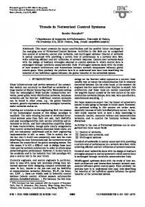
A block diagram of the discrete-time networked control system is shown in figure 1.
the power semi-norm of y can be computed through kykP =
s
Trace
µ
1 2π
Z
∞
Syy (ejω )dω −∞
In section 7, the positive and negative single-sided power spectral densities of a WSS process x are used, which are defined by the equations + (ejω ) Sxx
=
∞ X
Rxx [m]e−jmω
m=1 − (ejω ) Sxx
=
−1 X
Rxx [m]e−jmω
m=−∞
By the above definition, it follows that + − Sxx = Sxx + Sxx + Rxx [0]
Convergence in mean square sense is used in this paper. Refer to [11] for its definition. It can be shown [6] that a random vector process x = {x[n]} is convergent in mean square if and only if £ ¤ lim sup E (x[m] − x[n])T (x[m] − x[n]) = 0
n→∞ m≥n
A jump linear system is a linear dynamical system with random system matrices as follows. ½ x[n + 1] = A[n]x[n] + B[n]w[n] (2.1) y[n] = C[n]x[n] + D[n]w[n] where {A[n]}, {B[n]}, {C[n]}, and {D[n]} are matrix valued random processes. If the input process w[n] = 0, then we say that the system is a free jump linear system. A free jump linear system is said to be stochastically asymptotically stable¤ in mean square sense [7] £ if limn→∞ E x[n]T x[n] | x0 = 0 for any initial state x[0] = x0 . 1 Most
of the WSS processes in this paper are zero mean, so their covariances (auto-covariances) and correlations (autocorrelations) are equal. Therefore we interchangeably use these terms throughout the paper.
w
u
y
H( e jω ) _
e
- jω
d
×
_ y
Figure 1: The Control System with Data Dropouts In the system shown in figure 1, the loop function H(ejω ) is single-input single-out and strictly proper. w = {w[n]} is the exogenous input, which is wide sense stationary with zero mean. d = d[n] is the dropout process, which is independently identically distributed (i.i.d.) with probability distribution of Pr(d[n] = 1) = ε and Pr(d[n] = 0) = 1−ε. When d[n] = 0, y[n] = y[n], i.e. the measurement is sent sucessfully; when d[n] = 1, y[n] = y[n − 1], i.e. the measurement is dropped and the last measurement is reused. ε is the dropout rate. The dropout process d and the input process w are assumed to be independent. A state space representation of the system is ½ x[n + 1] = A[n]x[n] + Bw[n] y[n] = Cx[n]
(3.1)
where x is the state, {A[n]} is a random switching process. When d[n] = 0, A[n] = A0 ; when d[n] = 1, A[n] = A1 . Obviously {A[n]} is an i.i.d. matrix valued process with the probability distribution of Pr(A[n] = A1 ) = ε and Pr(A[n] = A0 ) = 1 − ε.
4 Wide Sense Stationarity In order to determine the power spectral density of the output process y = {y[n]}, we first need to show that the overall system in equation 3.1 is stable and y is wide sense stationary. This section states sufficient conditions for the stability of the overall system and the wide sense stationarity of y by the following theorems and corollaries. Their formal proofs will be found in section 7. Theorem 4.1 Consider the (free) jump linear system given in equation 3.1 with w = 0. Let A = {A[n]} be a matrix valued i.i.d. process such that Pr(A[n] = A1 ) = ε and Pr(A[n] = A0 ) = 1 − ε. Let the matrix X equal
(1 − ε)AT0 A0 + εAT1 A1 . The free jump linear system is stochastically asymptotically stable in the mean square sense if there exists a constant σX ∈ k otherwise
Based on the above expression, it can be shown by£ simply computations¤ that E [x[n + 1]] = 0 and E x[n + m + 1]xT [n + 1] is shift invariant with respect to n. So x = {x[n]} is wide sense stationary with zero mean. ♦ Proof of Theorem 5.1: Let the impulse response of H(ejω ) be h = {h[n]}. Because H(ejω ) is strictly proper, h[n] = 0 when n ≤ 0. So the output y can be expressed as y = h ∗ (y + w)
(7.1)
+ can be expressed as Then Syy + + Syy = D−1 Syy −
εe−jω Ryy [0] 1−ε
(7.8)
Syy is given by the equation − + Syy = Syy + Syy + Ryy [0]
(7.9)
Inserting the results of equations 7.7 and 7.8 into the above equation yields Syy
=
+ − + D−1 Syy D∗ Syy +
−
εe−jω Ryy [0] 1−ε
1 Ryy [0] 1 − εejω (7.10)
Combining equations 7.3 and 7.10 yields £ ¤∗ ³ + − ∗ Syy = D−1 ) − D−1 Syy − H(Syy + Syw ¶ 1 εe−jω Ryy [0] + Ryy [0] (7.11) jω 1 − εe 1−ε By the definition of the negative single-sided power £ − ¤∗ − + Syy spectral density, we know Syy = Syy + Ryy [0]. Inserting equation 7.11 into it yields £ ¤ £ ¤∗ ∗ ) + D−1 H ∗ (Syy + Syw ) Syy = D−1 H(Syy + Syw ¤∗ £ −1 ¤ £ Syy + ∆ D − D−1 (7.12) where ∆ =
1−ε2 (1−ε)2 Ryy [0]
−
2 1−ε Ryy [0]
+ Ryy [0].
Combining equations 7.4, 7.6 and 7.12, Syy yields Syy
=
¸· ¸∗ DH DH Sww 1 − DH 1 − DH ¸· ¸∗ · D D ∆ + 1 − DH 1 − DH
·
We then use the above result together with equations 7.4 and 7.6 to obtain the final expression of Syy . Syy
¯ ¯ ¯ ¯ ¯ H ¯2 ¯ DH ¯2 ¯ ¯ ¯ ∆ ¯ =¯ Sww + ¯ 1 − DH ¯ 1 − DH ¯
The last part deduces the algorithm for computing ∆. The direct computation of Ryy [0] shows that Ryy [0] = 2 Ryy [0]. So ∆ = 1−ε (Ryy [0] − Ryy [0]). By the definition of PSD, we get Z π ¢ ¡ 2 1 Syy (ejω ) − Syy (ejω ) dω ∆= 1 − ε 2π −π
Substitute the expressions of Syy (ejω ) and Syy (ejω ) into the above equation and we will get the final result of ∆.
References [1] Palopoli, L., L. Abeni, F. Conticelli, M. Di Natale, and G. Buttazzo, ”Real-time control system analysis: an ingetrated approach”, Real-Time Systems Symposium, 2000, pp. 131-140. [2] Ramanathan, P., ”Overload management in realtime control applications using (m, k)-firm gurantee”, IEEE Transactions on Parallel and Distributed Systems, Vol. 10 (1999), pp. 549-559. [3] Hamdaoui, M., and P. Ramanathan, ”A dynamic priority assignment technique for streams with (m, k)firm deadlines”, IEEE Transactions on Computers, Vol. 44 (1995), pp. 1443-1451.
[4] Beldiman, O., G.C. Walsh and L. Bushnell, ”Predictors for networked control systems”, Proc. 2000 American Control Conference, June 2000, pp. 23472351. [5] Walsh, G.C., O. Beldiman and L.G. Bushnell, ”Asymptotic behavior of nonlinear networked control systems”, IEEE Transactions on Automatic Control, vol. 46 (2001), pp. 1093-1097. [6] Wong, E. and B. Hajek, Stochastic Processes in Engineering Systems, Springer-Verlag, 1984. [7] Mariton, M., Jump Linear Systems in Automatic Control, Marcel Dekker Inc., 1990. [8] Nilsson, J., ”Real-time control systems with delays”, PhD thesis, Lund Institute of Tecnology, 1998. [9] Zhang, W., ”Stability analysis of networked control systems”, PhD Thesis, Case Western Reserve University, 2001. [10] Zhang, W., M.S. Branicky and S.M. Phillips, ”Stability of networked control systems”, IEEE Control Systems Magazine, vol. 21 (2001), pp. 84-99. [11] Stark, H., and J.W. Woods, Probability, Random Processes, and Estimation Theory for Engineers, Prentice Hall, Upper Saddle River, NJ, 1994, Second Edition.