Performance of Model-Based Networked Control Systems with ...

17th Mediterranean Conference on Control & Automation Makedonia Palace, Thessaloniki, Greece June 24 - 26, 2009

Performance of Model-Based Networked Control Systems with Discrete-Time Plants Panos J. Antsaklis∗

Tomas Estrada

Abstract

of the plant state were performed in instantaneous fashion, but with intermittent feedback the system remains in closed loop control mode for more extended intervals. This notion makes sense as it is a good representation of what occurs in both nature and industry. For example, when driving a car, when approaching a curve or hilly terrain, we pay attention to the road for a longer time, which is equivalent to staying in closedloop mode, and we only reduce our attention -switch to open loop control- when the road is once again straight. It is worth noting that while the application of intermittent feedback to MB-NCS is novel, the concept has been studied in a variety of fields such as [13], [23],[26], [14], [21]. While intermittent control is a very intuitive notion, its combination with the MB-NCS architecture allows for obtaining important results and opening new paths in controlling NCSs effectively.

In this paper we study performance-related aspects for plants in a networked control setting, employing an approach known as Model-Based Networked Control Systems (MB-NCS) with Intermittent Feedback. ModelBased Networked Control Systems use an explicit model of the plant in order to reduce the network traffic while attempting to prevent excessive performance degradation. Intermittent Feedback consists of the loop remaining closed for some time interval, then open for another interval. We begin by investigating the behavior of the system while tracking a reference input. We provide the full response of the system and a condition for stability. We then shift our attention to controller design for MB-NCS. We use dynamic programming techniques to design an optimal controller to optimize an LQ-like performance index.

In previous work [6, 7, 8], we have provided stability results for both the continuous and discrete setting. In this paper we shift our attention towards performance related aspects. We begin by considering an MB-NCS architecture with a reference input. In this architecture, the model receives its input directly from the controller, which is different from the plant’s input. We provide a full description of the state response of the system and a condition for stability. The results are derived for instantaneous feedback, but by taking τ = 0 they apply for the instantaneous feedback case as well. We then consider a discrete time MB-NCS without reference input and design an optimal controller to meet a linear quadratic-like performance index. Our methodology is based on the dynamic programming approach and is similar to that presented in [24] and [25].

1. Introduction A networked control system (NCS) is a control system in which a data network is used as feedback media. NCS is an important area in control, see for example recent surveys such as [2] and [11], as well as [23], [27], and [28]. The use of networks as media to interconnect the different components of an industrial system is rapidly increasing. However, the use of NCSs poses some challenges. One of the main problems to be addressed when considering an NCS is the size of the bandwidth required by each subsystem. A particular class of NCSs is model-based networked control systems (MB-NCS), introduced in [17]. The MB-NCS architecture makes explicit use of the knowledge of the plant dynamics to enhance the performance of the system. Here we extend this work by taking advantage of the concept of intermittent feedback. In the previous work done in MB-NCS, the updates given to the model

The rest of the paper is organized as follows. In Section 2, we investigate the behavior of MB-NCS model-based for the first architecture. We present the problem formulation in detail, derive the complete description of the state response and present a stability condition. In Section 3, we provide a method to design an optimal controller for an MB-NCS, by using dynamic programming techniques. Finally, in Section 4, we provide conclusions and propose future work.

∗ T. Estrada and P.J. Antsaklis are with the the Department of Electrical Engineering, University of Notre Dame, Notre Dame, IN 46556, USA. E-mail: {testrada,antsaklis.1}@nd.edu

978-1-4244-4685-8/09/$25.00 ©2009 IEEE

628

Authorized licensed use limited to: UNIVERSITY NOTRE DAME. Downloaded on October 6, 2009 at 17:11 from IEEE Xplore. Restrictions apply.

2. Discrete-time MB-NCS with Intermittent feedback and Reference Input

closed for τ seconds, and the system runs open loop for a period of τ − h seconds. Recall that in the discrete time case, τ and h are both integers. Let us first consider what happens during the open loop interval, that is, when n ∈ [nk + τ , nk+1 ). For this interval, we have that

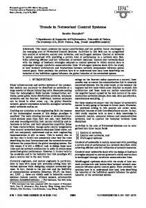
We will presently study the behavior of an MBNCS with instantaneous feedback, introducing a reference input signal r. We will consider two cases, differing from each other in the implementation of the input to the model. The first one is depicted in the following figure.

u = K xˆ − r

(1)

so 

x (n + 1) xˆ (n + 1)





A 0

BK = ˆ Aˆ + BK   −B r + −Bˆ



x(n) x(n) ˆ



(2)

with initial conditions x(n ˆ k + τ ) = x (nk + τ ). Rewriting in terms of x and e, that is, of the vector z:      A + BK −BK x(n) x (n + 1) z(n) = = ˜ ˜ ˜ e(n) e (n + 1) A + BK Aˆ − BK   −B + r (3) −B     x(nk ) x(nk − ) z(nk ) = = , ∀n ∈ [nk + τ , nk+1 ) e(nk ) 0 Thus, we have Figure 1. Basic MB-NCS architecture z (n + 1) = Λo z (n) + Ψr (n) ,   A + BK −BK where Λo = ˜ ˜ ˜ A + BK Aˆ − BK   −B and Ψ = , ∀n ∈ [nk + τ , nk+1 ) −B

In this architecture, the model receives its input directly from the controller, which is different from the plant’s input. This corresponds to a situation where the model is collocated with the controller and set in a remote access location.

(4)

For the closed loop case, similarly we obtain z (n + 1) = Λc z (n) + Ψr (n) ,   A + BK −BK where Λc = 0 0   −B and Ψ = , ∀n ∈ [nk , nk + τ ) −B

2.1. State response of the system The plant is given by x(n + 1) = Ax(n) + Bu(n), the plant model by x(n ˆ + 1) = Aˆ xˆ (n) + Bˆ uˆ (n). The controller is linear state feedback, with the difference that while the input to the controller is still uˆ (n) = K xˆ (n) , the input to the plant is now given by u (n) = K xˆ (n) − r (n). The state error is defined as e = x− xˆ and represents the difference between plant state and the model state. The modeling error matrices A˜ = A − Aˆ and B˜ = B − Bˆ represent the plant and the model. We also define the vector z (n) = [xT eT ]T . We will now proceed to derive the response and later summarize the result in a proposition. As in the case without reference input studied in [6], the error is reset every h seconds, the loop remains

(5)

From this, it should be quite clear (by solving the difference equation) that given an initial condition z(n = 0) = z0 , then after a certain time n ∈ [0, τ ), during which the system has been running in close loop, the solution of the trajectory of the vector is given by n−1

z(n) = Λnc z0 + ∑ Λnc z j+1 Ψr ( j) , n ∈ [0, τ ).

(6)

j=0

Notice that this evidently can be expressed as the sum of two terms, a ”zero-input response” and a ”zerostate response”.

629 Authorized licensed use limited to: UNIVERSITY NOTRE DAME. Downloaded on October 6, 2009 at 17:11 from IEEE Xplore. Restrictions apply.

and similarly for for n ∈ [nk , nk + τ ).

Similarly, for the first open loop interval, the solution of the trajectory is given by

We can combine what we have developed for zerostate and zero-input and summarize the results in the following proposition.

n−1

z(n) = Λon−τ z (τ ) + ∑ Λon−τ z j+1 Ψr ( j) , n ∈ [τ , h) (7) j=τ

Proposition 1 Thesystem described by (4) with initial  x (t0 ) conditions z (t0 ) = = z0 has the following re0 sponse:

Notice that this, too, can be expressed as the sum of a ”zero-input response” and a ”zero-state response”. We will thus continue the derivation by focusing first on what happens to the zero-input response, then to the zero-state response. The zero-input response is identical to that which we had in the case without reference input, described in [8]. After k cycles, going through this analysis yields a solution  k   I 0 I 0 z0 z (nk ) = Λo (h − τ )Λc (τ ) 0 0 0 0

z(n) = Λc (n − nk ) k−1





k−1

+∑ l=0

+∑

l=0



n +h−1

τ l Λh− ∑ j=n o z j+1 Ψr ( j) l +τ nl +τ −1 τ + ∑ j=nl Λc z j+1 Ψr ( j)

!

k (8)



I 0

0 0



n +h−1

τ l Λh− ∑ j=n o z j+1 Ψr ( j) l +τ nl +τ −1 τ Λc z j+1 Ψr ( j) + ∑ j=n l

!!

Having written the state response of the system, we can easily see that we can arrive at a BIBO stability condition. This condition would be the same as the condition for global exponential stability in the case without reference input. This can be clearly seen from the fact that by bounding the input, the zero-state part of the solution will also be bounded, so we need only that the stability of the zero-input part be stable, and this has been done in previous work. We include the theorem here for completeness. Theorem 2 The system described  by  above is BIBO x stable around the solution z = if and only if the e    I 0 I 0 eigenvalues of Σ are strictly inside 0 0 0 0 the unit circle, where Σ = Λo (h − τ )Λc (τ ). The proof can be found in [8]. The results can be extended to other reference input architectures, as in [9]. Also, while we have considered intermittent feedback, the results also apply to the instantaneous feedback case by specifying τ = 0. In the next section, we will focus on the instantaneous feedback case to design a controller for a discrete time MB-NCS.

j=0

I 0 0 0

I 0 0 0

2.2. BIBO stability condition

kz j+1 Ψr ( j) ∑ Λn−n c

k−1 

Λo (h − τ )Λc (τ )



for n ∈ [nk , nk + τ ),with nk+1 − nk = h, k =1, 2, 3...,  A + BK −BK −B , and Ψ = . where Λo = ˜ ˜ ˜ −B A + BK Aˆ − BK The result is similar for n ∈ [nk + τ , nk + 1) and is omitted for reasons of space.



k−1

z (n) =



j=0

I 0 I 0 Λo (h − τ )Λc (τ ) . 0 0 0 0 The final step is to consider the last (partial) cycle that the system goes through, that is, the time n ∈ [nk , nk+1 ). If the system is in closed loop, that is, n ∈ [nk , nk + τ ), then the solution can be achieved merely by pre-multiplying z (nk ) by Λc (n − nk ) . In the case of the system being in open loop, that is, n ∈ [nk + τ , nk+1 ), then clearly we must pre-multiply by Λo (n − (nk + τ )) Λc (τ ) . Now, the zero-state term will experience a similar evolution. At time τ , the value of the zero-state part will be −1 τ Λc z j+1 Ψr ( j) . ∑τj=0 Unlike the case with the zero-input case, the portion from the next time interval, rather than premultiplied, will rather be added to this term. So at time h, the value of the zero-state part wil be τ −1 τ h−τ ∑h−1 j=τ Λo z j+1 Ψr ( j) + ∑ j=0 Λc z j+1 Ψr ( j) . Notice that the error portion of the term will have to be reset at each nk, which corresponds to preI 0 multiplying by . 0 0 We continue the add the portion from the next time interval and do so again for k cycles to obtain: where Σ =

0 0

I 0

kz + ∑ Λn−n j+1 Ψr ( j) c

= Σk z0 ,





,

for n ∈ [nk , nk + τ ), with nk+1 − nk = h, k = 1, 2, 3...

630 Authorized licensed use limited to: UNIVERSITY NOTRE DAME. Downloaded on October 6, 2009 at 17:11 from IEEE Xplore. Restrictions apply.

z0

3. Controller design of MB-NCS using optimal control techniques

Our procedure follows that of (24) in that we define a cost-to-go function and calculate it iteratively. To begin, observe that the equations of the system can be rewritten as:

Let us now consider a system with a discrete-time linear time-invariant plant, where the full information of the state of the plant is only available with probability v. ¯ We will consider the case without a reference input in this section. When the state of the plant is not available, the model is used to compute the control action. Our main objective is to find a controller that will optimize an LQ-based performance criterion for this system and to compute this optimal cost as well. The setup is as follows. We will consider the discrete-time plant governed by: xk+1 = Axk + Buk

xk+1 = (A + vk BK)xk + (1 − vk )BK xˆk ˆ k + [Aˆ + (1 − vk)BK] ˆ xˆk xˆk+1 = vk BKx uk = vk Kxk + (1 − vk)K xˆk

T  Let us define z = xTk xˆTk . We can thus write the equations concerning the plant and model state as zk+1 = F (νk ) z, where: F (νk ) =

(9)

The equations of the model are given by: ˆ k xˆk+1 = Aˆ xˆk + Bu

CkN (zk ) = E



(15)

"

N

∑

xTk Qxk + uTk Ruk

h=k

#

(16)

(11) where Qk = Q and Rk = R except for the terminal cost RN = 0. Following the standard procedure in these cases, we make the claim that this function can be written as CkN (zk ) = E [zk Sk zk |zk ] ,

ˆ B, ˆ are the and where A, B are the plant matrices, A, model matrices, uk is the input, x is the state of the plant, x is the state of the model, and K is the controller. Also, ek = xk − xˆk denotes the error between the plant state and model state. Notice that the above expressions capture a situation where, if the actual state of the plant is available, that value is used to calculate the control law, but, if it is not available, then the control input is calculated by using the state of the model. Notice also that this corresponds to the case τ = 0, as we might have cases where we have access to the plant for a single clock instant only. We use the expected total cost as our performance index: " #

(17)

which is clearly true for k = N and SN = Q. Then, by induction, we show this is true for all k. Suppose it is true for k + 1, then: CkN (zk )

=E

"

N

∑

xTk Qxk + uTk Ruk |zk

#

(18)

h=k   T N |zk = E xk Qxk + uTk Ruk + Ck+1 [xT Qx +  T k k vk Kxk + =E R (vk Kxk + (1 − vk)K xˆk ) (1 − vk )K xˆk N |z ] +Ck+1 k T [z k   Q + v2k K T RK (1 − vk ) vk K T RK zk =E (1 − vk ) vk K T RK (1 − vk )2 K T RK T T +zk F (vk ) Sk+1 F (vk ) zk |zk ]   Q + vK ¯ T RK 0 T zk [zk 0 vK ¯ T RK

∞

∑ xTk Qxk + uTk Ruk

(A + vk BK) (1 − vk )BK ˆ ˆ vk BK [Aˆ + (1 − vk)BK]

The cost-to-go function Ck is defined as follows:

where the probability of having access to the full state of the plant is governed by the stochastic variable vk , with  1 , with probability v¯ vk = (12) 0 , with probability 1 − v¯

J∞ = E



(10)

and the control input is given by uk = K xˆk + vk Kek

(14)

(13)

k=0

We will design an optimal controller K to optimize this performance index. The matrices Q and R are selected by the user according to the performance objective desired, with Q penalizing the system for high values in the state of the plant and R doing so for using excessive control effort.

=E

+vz ¯ Tk F T (0) Sk+1 F (0)zk +(1 − v¯)zTk F T (1) Sk+1 F (1) zk |zk ]

(19)

Therefore, the above claim is true, and, moreover, we

631 Authorized licensed use limited to: UNIVERSITY NOTRE DAME. Downloaded on October 6, 2009 at 17:11 from IEEE Xplore. Restrictions apply.

with

can write that (20)

Sk 

Q + vK ¯ T RK

T −1 Ψ (S1 ) = P1 − P12 P2 P12



0 = + (21) 0 vK ¯ T RK     A BK AT 0 S + v¯ k+1 ˆ 0 Aˆ + BK K T BT Aˆ + K T Bˆ T     A + BK 0 (A + BK)T K T Bˆ T + (1 − v¯) Sk+1 ˆ BK Aˆ 0 Aˆ T

KS = −P2−1 P12

Ψ (S1 ) ≤ L (K, S1 ) , ∀K where the operator Ψ (S1 ) is nonlinear in S1 . The condition P2 > 0 is necessary for stability because, were it not met, we could select K such that it would yield a nonpositive definite S1 , which is not feasible. The previous inequality can be used to find an optimal gain K that minimizes the matrix S1 .

where the operator F (Sk+1 , K) is affine in S for fixed K, and quadratic in K for fixed S. To obtain the infinite horizon cost, we take the limit as time goes to infinity of the cost-to-go function. N→∞

(22) Theorem 3 Consider the system defined by (10)-(12) and the infinite horizon cost defined in (13). Assume that the pairs (A, B) and (AT , Q1/2 ) are stabilizable. Then the optimal infinite horizon cost J∞ = minL J∞ (K) is given by J∞∗ = xT0 T∞∗ x0 where T∞ is the unique strictly positive solution of the equation:

where S∞ is the solution of the Lyapunov-like equation S∞ = F (S∞ , K) , if the solution exists. Let us now partition the matrix S∞ as follows   S1 S12 . (23) S∞ = S1T S2 Then the Lyapunov-like equation S∞ = F (S∞ , K) can be expanded as:

T∞∗ = Ψ (T∞∗ ) where Ψ (T ) is defined in (6.34) and the optimal gain is given by K ∗ = KT∞∗

S1 = Q + vK T RK + vAT S1 A+ (24)   T (A + BK) S1 (A + BK)+ T (A + BK)+ , K T Bˆ T S12 (1 − v)  T (A + BK) S12 BK + K T Bˆ T S2 BK   ˆ + S12 = v AT S1 BK + AT S12 Aˆ + AT S12 BK   (1 − v) (A + BK)T S12 A + K T Bˆ T2 SA ,

(28)

If P2 > 0, then

= F (Sk+1 , K) ,

J∞ (K) = lim C0N (x0 ) = xT0 S∞ x0

(27)

with KS as defined in (28). The equation T∞∗ = Ψ (T∞∗ ) has a positive definite solution if and only if v¯ > vc , where vc is a critical probability of having access to the ˆ B). ˆ channel, which depends on the pairs (A, B) and (A, The T∞∗ can be obtained as the limit of the sequence Tk+1 = Ψ (Tk ), that is, limk→∞ Tk = T∞ .

(25)

S2 = vK T RK+  T T  T BK K B S1 BK + (Aˆ T + K T Bˆ T )S12 + v +K T BT S12 (Aˆ + BK)+ T ˆ ˆ (A + BK) S2 (A + BK) T (1 − v)Aˆ S2 Aˆ . (26)

4. Conclusions and future work In this paper, we investigated the behavior of the system while following a reference input. We provided the full response of the system and a stability condition. We then designed an optimal controller for MB-NCS to meet an LQ-like performance index, by using dynamic programming techniques. Some extensions of these results can be found in [9] and will continue to be developed in future work. Additionally, we will seek to use intermittent feedback to improve performance, by updating the model during the times when the system is running closed loop, with the aim of enabling the user to run the system closed loop for progressively shorter intervals.

Via algebraic manipulations, we can express all of the above in terms of S1 . Furthermore, the resulting S1 equation is the only one that depends on the control gain K and can be written as: T K + K T P12 + K T P2 K = L (K, S1 ) S1 = P1 + P12

with P1 , P12 , P2 all linear functions of the matrix S1 for fixed K. We can also write T −1 L (K, S1 ) = P1 − P12 P2 P12

+ (K + P2−1P12 )T P2 (K + P2−1P12 ) = Ψ (S1 ) + (K − KS )T P2 (K − KS )

632 Authorized licensed use limited to: UNIVERSITY NOTRE DAME. Downloaded on October 6, 2009 at 17:11 from IEEE Xplore. Restrictions apply.

References [17]

[1] P. Antsaklis and A. Michel, Linear Systems, 1st edition, McGraw-Hill, New York, 1997. [2] J. Baillieul, P. Antsaklis. ”Control and communication challenges in networked real-time systems,” Proceedings of the IEEE, v 95, n 1, Jan. 2007, p 9-28. [3] B. Azimi-Sadjadi, ”Stability of Networked Control Systems in the Presence of Packet Losses,” Proceedings of the 42nd Conference of Decision and Control, December 2003, pp. 676- 681. [4] M.S. Branicky, S. Phillips, and W. Zhang, ”Scheduling and feedback co-design for networked control systems,” Proceedings of the 41st Conference on Decision and Control, December 2002, pp. 1211- 1217. [5] D. Delchamps, ”Stabilizing a Linear System with Quantized State Feedback,” IEEE Transactions on Automatic Control, vol. 35, no. 8, pp. 916-924. [6] T. Estrada, H. Lin, and P.J. Antsaklis, ”Model-Based Control with Intermittent Feedback”, Proceedings of the 14th Mediterranean Conference on Control and Automation, 2006, pp. 1-6. [7] T. Estrada and P.J. Antsaklis, ”Control with Intermittent Sensor Measurements: A New Look at Feedback Conrol”, Proceedings of the Workshop on Networked Distributed Systems for Intelligent Sensing and Control, Athens, Greece, 2007. [8] T. Estrada and P.J. Antsaklis, ”Results on Continuous and Discrete Model-Based Networked Control Systems with Intermittent Feedback, Part I: Stability.”, ISIS Technical Report ISIS-2008-001, April 2008. [9] T. Estrada and P.J. Antsaklis, ”Results on Continuous and Discrete Model-Based Networked Control Systems with Intermittent Feedback, Part II: Performance.”, ISIS Technical Report, April 2009. [10] E. Fridman, A. Seuret, J.P. Richard, “Robust sampleddata stabilization of linear systems: an input delay approach”, Automatica, 2004. [11] J. Hespanha, P. Naghshtabrizi, Yonggang Xu, ”A survey of recent results in networked control systems”, Proceedings of the IEEE, v 95, n 1, Jan. 2007, p 138-62. [12] D. Hristu-Varsakelis, ”Feedback Control Systems as Users of a Shared Network: Communication Sequences that Guarantee Stability,” Proceedings of the 40th Conference on Decision and Control, December 2001, pp. 3631-36. [13] M. Kim, et al, ”Controlling chemical turbulence by global delayed feedback:Pattern formation in catalytic co oxidation” on pt(110), Science, vol. 292, no. 5520, 2001. [14] K. Koay and G. Bugmann, ”Compensating intermittent delayed visual feedback in robot navigation”, Proceedings of the IEEE Conference on Decision and Control, 2004. [15] D. Liberzon and R. Brockett, ”Quantized Feedback Stabilization of Linear Systems,” IEEE Transactions on Automatic Control, Vol 45, no 7, pp 1279-89, July 2000. [16] L.A. Montestruque, PhD Dissertation, Model-Based

[18]

[19]

[20]

[21]

[22]

[23]

[24]

[25]

[26] [27]

[28]

Networked Control Systems, University of Notre Dame, Notre Dame IN, USA, September 2004. L.A. Montestruque and P.J. Antsaklis, ”Model-Based Networked Control Systems: Necessary and Sufficient Conditions for Stability”, 10th Mediterranean Conference on Control and Automation, July 2002. L.A. Montestruque and P.J. Antsaklis, ”State and Output Feedback Control in Model-Based Networked Control Systems”, 41st IEEE Conference on Decision and Control, December 2002, pp. 1620- 1625. L.A. Montestruque and P.J. Antsaklis, ”On the modelbased control of networked systems,” Automatica, Vol. 39, pp 1837-1843. L.A. Montestruque and P.J. Antsaklis, ”Networked Control Systems: A model-based approach,” 12th Mediterranean Conference on Control and Automation, June 2004. E. Ronco and D. J. Hill, ”Open-loop intermittent feedback optimal predictive control:a human movement control model”, NIPS99, 1999. G. Nair and R. Evans, ”Communication-Limited Stabilization of Linear Systems,” Proceedings of the Conference on Decision and Control, 2000, pp. 1005-1010. B. H. Salzberg, A. J. Wheeler, L. T. Devar, and B. L. Hopkins, ”The effect of intermittent feedback and intermittent contingent access to play on printing of kindergarten children”, J Anal Behav, vol. 4, no. 3, 1971. L. Schenato. “To zero or to hold control inputs in lossy networked control systems”, Proceedings of the European Control Conference, Kos, Greece, 2007. L. Schenato, B. Sinopoli, M. Franceschetti, K. Poolla, and S. Sastry. “Foundations of Control and Estimation over Lossy Networks.“ Proceedings of the IEEE, Special Issue on Networked Control Systems. Vol. 95, Issue 1, January 2007. Richard A. Schmidt, Motor Control and Learning - A Behaviorial Emphasis. Human Kinetics, 4th ed., 2005. J. Took, D. Tilbury, and N. Soparkar, ”Trading Computation for Bandwidth: Reducing Computation in Distributed Control Systems using State Estimators,” IEEE Transactions on Control Systems Technology, July 2002, Vol 10, No 4, pp 503-518. G. Walsh, H. Ye, and L. Bushnell, ”Stability Analysis of Networked Control Systems,” Proceedings of American Control Conference, June 1999.

633 Authorized licensed use limited to: UNIVERSITY NOTRE DAME. Downloaded on October 6, 2009 at 17:11 from IEEE Xplore. Restrictions apply.