Journal of Modern Physics, 2014, 5, 353-358 Published Online April 2014 in SciRes. http://www.scirp.org/journal/jmp http://dx.doi.org/10.4236/jmp.2014.56045
Role of the Reference Frame in Angular Photon Distribution at Electron-Positron Annihilation Andrey N. Volobuev, Eugene S. Petrov, Eugene L. Ovchinnikov Department of Physics, Samara State University, Samara, Russia Email:
[email protected] Received 14 February 2014; revised 13 March 2014; accepted 11 April 2014 Copyright © 2014 by authors and Scientific Research Publishing Inc. This work is licensed under the Creative Commons Attribution International License (CC BY). http://creativecommons.org/licenses/by/4.0/
Abstract The reasons of angular photon distribution occurrence at electron-positron annihilation are considered. It is shown that angular photon distribution is consequence of Doppler’s effect in the reference frame of the electron and positron mass center. In the reference frame bound with moving electron the angular photon distribution is absent. But it is replaced by the Doppler’s shift of photons frequencies. The received results are applied to the analysis of a positron-emission tomograph work.
Keywords Annihilation, Electron, Positron, Photon, Doppler’s Effect, Angular Photon Distribution, Positron-Emission Tomograph
1. Introduction The analysis of angular distribution of flying out photons at annihilation a positron and electron has great importance for designing positron-emission tomographs (PET). PET is the advanced diagnostic device used for search new growth at the earliest stages of their occurrence. Unfortunately the mechanism of annihilative process of the electron and positron is unknown. P. Dirac has been offered model of this process. According to Dirac [1] [2] for the annihilation it is possible to present as transformation of the electron from a state with positive energy to the state with negative energy. According to the Dirac theory vacuum holes, the positron is holed in the field of vacuum. Interaction of the electron and positron i.e. the annihilation is a filling vacuum hole by the electron. Thus energy as two quantums of electromagnetic radiation is allocated. How to cite this paper: Volobuev, A.N., et al. (2014) Role of the Reference Frame in Angular Photon Distribution at Electron-Positron Annihilation. Journal of Modern Physics, 5, 353-358. http://dx.doi.org/10.4236/jmp.2014.56045
A. N. Volobuev et al.
2. The Angular Photon Distribution at Electron-Positron Annihilation Quantum-electrodynamical calculations of the annihilative process have been carried out enough for a long time. They were repeatedly checked and rechecked, including authors of the article. As a result of these calculations two formulas for the differential effective section of electromagnetic radiation quantums scattering in a solid angle dΩ have been found. The first formula on time has been found by Heitler [2]. This formula looks like: 0 2 + p 2 + p 2 sin 2 θ k = − dσ 2 2 4 ( 4π ) k 0 p k 0 − p 2 cos 2 θ
( ) ( )
e4
((
dΩ . 2 2 0 2 2 − p cos θ k 2 p 4 sin 4 θ
)
)
(1)
The formula is written in designations [3] where there is its detailed deduction. The so-called rational system of units which speed of light and Planck’s constant are equal to unit c= = 1 is used. In this system the units of energy, impulse and weight have the same dimension. In the formula (1) e there is electron charge (or positron with an opposite sign), k 0 ―the photon energy, p ―the electron impulse, θ ―the angle between impulses of the electron and one of the radiated photons. Formula (1) is found under condition of summation on all directions of photons polarization. At the deduction (1) the reference frame connected to the center of mass interacting the electron and positron is used which the impulses of electron and positron are equal on the module and are opposite on the direction p1 = − p2 = p . Impulses of photons also are equal on the module and opposite on the direction k1 = −k2 [2] [3]. We shall note that in this reference frame of the condition of both photons supervision are identical. The second formula has been offered a little later by Feynman [4]:
= dσ
ω1 ω2 e 4ω12 2 + 2 − 4 ( e1e2 ) dΩ . + 64π 4m p+ ( E+ + m ) ω2 ω1 2
2
(2)
The formula (2) is written down in designations [4]. As well as in the previous variant (1) the rational system of units is used. In the formula (2) e1 and e2 there are individual vectors of photons polarization radiated at annihilation, ω1 and ω2 ―the frequencies of the radiated photons, m ―the mass of electron (or positron), p+ ―the module of the positron impulse, E+ ―its energy. The formula (2) is similar to Klein-Nishina formula for Compton effect [4] [5]. The main difference there are before the third and fourth addends in the square brackets the signs are changed on opposite. The major distinctive condition of Formula (2) deduction is use of other reference frame in comparison with Formula (1) deduction. Formula (2) was deduced in the reference frame in which electron is at rest, and positron moves. This reference frame as a whole is equivalent to the reference frame connected with PET. Therefore we shall name this reference frame―laboratory. The electrons in the object researched in PET basically are in the bound state. Positrons are result β ―positron radioactive decay of elements. Therefore electrons in laboratory reference frame it is possible to assume motionless (if to exclude chaotic thermal movement of molecules). Both formulas (1) and (2) were deduced with the help of standard diagram technique of Feynman and diagrams of the perturbance theory of second order. However results of the deductions essentially differ. First, the formula (1) assumes rather complex angular distribution of annihilative photons. And this distribution is connected only to the electron impulse. The angle θ is present only at the complex with impulse p . In Formula (2) the angular distribution of photons is absent. Second, Formula (2) assumes the opportunity of photons various energy at annihilation that is forbidden by Formula (1) deduction owing to k1 = −k2 . Therefore, first of all, there is a question what nature of angular distribution of the annihilative photons in (1)? Whether this distribution with annihilative process i.e. transformation “substance-energy” is connected or that is defined by other effects? Whether the given angular distribution of photons will be kept at transition to other reference frame, for example, bound with PET?
354
A. N. Volobuev et al.
3. The Reason of Photons Angular Distribution
For research of the angular dependence reason of differential effective section (1) we shall consider intermediate expression of the deduction which is not summarized yet on directions of the photons polarization [3]:
( )
( ) ( e e )( pe )( pe ) −
( )
4 4 2 2 k0 4 k 0 ( pe1 ) ( pe2 ) 4 k0 1 e4 dσ = − − 2 2 128π 2 pk 0 ( pk1 )( pk2 ) ( pk1 ) ( pk2 )
2
1 2
1
( pk1 )( pk2 )
2
( e1e2 )
2
dΩ ,
(3)
where k1 and k2 there are impulses of photons. Variables in square brackets: an impulse of electron, impulses of photons, unit vectors of photons polarization are written down as 4-vectors. Formula (3) is simple for transforming to the kind:
( )
4 2 k0 e4 1 0 2 ( pe1 )( pe2 ) (4) = − + k e e dσ 2 ( ) dΩ . 128π 2 pk 0 ( pk1 )( pk2 ) ( pk1 )( pk2 ) 1 2 0 0 ab ) a b − ab where a and b there are three-dimenLet’s transit in (4) to spatial vectors using a rule (= sional vectors which components change covariance, a 0 and b0 ―contravariance changing components of 4vectors, in our case power components. Transiting to three-dimensional vectors, and also taking into account absence contravariance components at polarizing 4-vectors e0 = 0 the expression (4) it is possible to present as:
( )
2 4 k0 2 pe pe ( )( ) 1 e4 1 2 = − 2 k 0 + ( e1e2 ) dΩ dσ 2 0 4 128π 2 pk 0 k 0 4 − ( pk )2 k − ( pk1 ) 1 2 2 ( pe1 )( pe2 ) 1 e 4 1 = − + ( e1e2 ) dΩ. 2 0 2 2 2 128π pk k0 pk1 1 − pk12 1− 2 k0 k0
( )
( )
( )
( )
(5)
( )
( )
( )
At the deduction (5) the condition of photons flying in strict opposite directions k2 = −k1 also is used. Taking into account k1 = k 0 , and also according to the energy conservation law сk 0 = mc 2 (for clearly pk1 V = cos θ , evident it is entered inside brackets speed of light с = 1 ) in the formula (5) we shall replace 0 2 c k
( )
where V ―speed of electron. In result we shall receive: 2 pe pe ( )( ) e4 1 1 2 1 2 = − + ( e1e2 ) dΩ . dσ 2 2 2 0 128π 2 pk 0 V V k 1 cos θ 1 − cos θ − c c
( )
(6)
Let’s transit in (6) to the laboratory reference frame offered in [4], and bound with electron. In this case p = 0 , and V it is possible to examine as speed of a positron movement. The same there concerns and to value p in factor before brackets. In the given reference frame the formula (6) becomes simpler:
1 e 1 2 e e = dσ − ( 1 2 ) dΩ . 2 128π 2 pk 0 V 1− cos θ c 4
355
(7)
A. N. Volobuev et al.
We research an auxiliary task. The observer 1 who are taking place in “motionless” (connected with the Earth) reference frame, Figure 1, examines some particle 2 moving with a speed V which in certain moment of time radiates two opposite directed quantums. At V = 0 the quantum frequency is ω0 . The angle between speed of the particle and direction of one quantum propagation is equal θ . In the observer direction the particle has a component of speed V cos θ . Due to Doppler’s effect the quantum moving in the observer direction will have the increased frequency [6]: 1−
ω1 = ω0
1−
V2 c2
V cos θ c
.
(8)
For the quantum moving in an opposite direction so-called the “red displacement” of frequency will be observed: 1−
ω2 = ω0
1+
V cos θ c
.
(9)
ω1 ω2 + + 2 which is included into the formula (2): ω2 ω1
Using (8) and (9) we shall find size of the complex
(ω1 + ω2 )
ω1 ω2 += +2 ω2 ω1
V2 c2
2
=
ω1ω2
4 V 1 − cos θ c
2
.
(10)
Let’s note that distinction in frequencies of quantums in an examined task is determined by distinction in conditions of these quantums supervision: one quantum moves to the observer another leaves from him. In Formula (7) the considered auxiliary task is actually realized. Thus the moving particle is meant as a positron, and the observer is on “motionless” electron. Therefore substituting (10) in (7) we shall find:
= dσ
1 e4 128π 2 pk 0
2 1 ω1 ω2 + + 2 − ( e1e2 ) dΩ 4 ω2 ω1
1 e4 = 128π 2 4 pk 0
(11)
ω1 ω2 2 + 2 − 4 ( e1e2 ) dΩ + ω2 ω1
Let’s note that at use of Formula (10) we have actually refused the condition k2 = −k1 . If in factor before brackets in Formula (2) to use E+= m= ω1 Formulas (2) and (11) become identical. In summary we shall summarize the formula (11) on photons polarization. Coming back to polarizing 4-vectors with the account e0 = 0 also using
∑ ( e1e2 )
2
= 2 [3], we shall find:
e1 , e2
1
V ω2
θ
2
ω1
Vcosθ
Figure 1. Supervision of the photons which be emitted by the moving particle.
356
1 e 4 ω1 ω2 2 + + 2 − 4 ( e1e2 ) dΩ 2 0 128π 4 pk ω2 ω1 2 1 e 4 (ω2 − ω1 ) = 1− dΩ 4ω1ω2 128π 2 pk 0
A. N. Volobuev et al.
= dσ
(12)
The sign on the module is written owing to standard use of the compound matrix element module at finding of the differential effective section of process [2]. Taking into account that in the positron-emission tomograph the speeds of positrons are small, and also taking into account (8) and (9) it is possible to write down: V2 c2 = ω1ω2 ω02 ≈ ω02 . 2 V 1 − cos 2 θ c 1−
(13)
Substituting (13) in (12) we shall receive: dσ ≈
e4 1 128π 2 pk 0
( ∆ω )2 1− 4ω02
dΩ ,
(14)
where it is designated ∆ω = ω2 − ω1 . On Figure 2 the basic scheme of photons registration in the positron-emission tomograph [7] is shown. The researched object 2 is located in the ring of detectors 1. At the annihilation of the positron and electron which is in a point a the two quantums with energies ω1 and ω2 in opposite directions flying out. If the quantums flying on line A-A are registered by detectors D1 and D2 simultaneously the point of quantums emission is in the middle between detectors D1 and D2 . Detectors in the ring 1 from the point of Doppler’s effect view in the reference frame bound with electron have a role of motionless observers. By the number of the quantums which are flying in different directions the process it is spherical-symmetrically. Therefore the density of detectors in the ring 1 should be uniform. However the quantum frequencies and consequently also their energy depending on the detector direction (observer) due to Doppler’s effect can differ on size ∆ω = ω2 − ω1 .
4. Conclusions By results of the carried out analysis we can draw the following conclusions. Formulas Heitler (1) and Feynman (2) it is adequate in different reference frames to describe scattering photons at annihilation of electron and positron. 1
D1
ω1
A
ω2
D2
a
θ
2
Figure 2. The basic scheme of photons registration in the positron-emission tomography.
357
A. N. Volobuev et al.
In the laboratory reference frame bound with electron the angular distribution of number photons is absent however due to distinction in conditions of quantums supervision there is a distinction in frequencies of the radiated quantums (owing to Doppler effect). At transition in the reference frame bound to the center of mass of electron and positron the distinction in frequencies of the radiated quantums is reduced in angular distribution of photons which is also consequence of Doppler’s effect. In the laboratory reference frame bound to the positron-emission tomographs radiation of the annihilative quantums by number is spherical-symmetrically however it is necessary to take into account some distinction of the opposite radiated photon frequencies.
References [1]
Dirac, P.A.M. (1978) Direction in Physics. Edited by H. Hora and J. R. Shepanski, John Wiley & Sons, New York.
[2]
Heitler, W. (1956) Quantum Theory of Radiation. In. Lit., Moscow, 302-304.
[3]
Bogolubov, N.N. and Shirkov, D.V. (1976) Introduction in the Theory of Quantum Fields. Science, Moscow, 203-205.
[4]
Feynman, R.P. (2009) Quantum Electrodynamics, A Lecture Note. Book House LIBROKOM, Moscow, 135-137.
[5]
Volobuev, A.N., Petrov, E.S. and Ovchinnikov, E.L. (2012) Journal of Modern Physics, 3, 585-596.
[6]
Landay, L.D. and Lifshits, E.M. (1967) Theory of Field. Science, Moscow, 156.
[7]
Volobuev, A.N. (2011) Bases of Medical and Biological Physics. Samara Publishing House, Samara, 636.
358