Sample Covariance Matrix Eigenvalues Based Blind

Sample Covariance Matrix Eigenvalues Based Blind SNR Estimation Mohamed Hamid ∗† , Niclas Bj¨orsell ∗ , and Slimane Ben Slimane † ∗ University of G¨ avle, 801 76 G¨avle, Sweden † Wireless@kth, Communications Systems Lab (CoS), The Royal Institute of Technology (KTH), 164 40 Stockholm, Sweden

Abstract—In this paper, a newly developed SNR estimation algorithm is presented. The new algorithm is based on the eigenvalues of the sample covariance matrix of the recieved signal. The presented algorithm is blind in the sense that both the noise and the signal power are unknown and estimated from the received samples. The Minimum Descriptive Length (MDL) criterion is used to split the signal and noise corresponding eigenvalues. The experimental results are judged using the Normalized Mean Square Error (NMSE) between the estimated and the actual SNRs. The results show that, depending on the value of the received vectors size and the number of received vectors, the NMSE is changed and down to -55 dB NMSE can be achieved for the highest used values of the system dimensionality. Index Terms—SNR estimation, Sample covariance matrix, Eigenvalues detection, Minimum Descriptive Length criterion (MDL).

I. I NTRODUCTION Precise signal-to-noise-ratio (SNR) estimation is of a great importance in wireless systems as many algorithms are SNR dependant. Examples for such algorithms are: linear diversity combining techniques [1] and link adaptation algorithms techniques such as adaptive modulation and coding [2]. There exist many SNR estimation techniques which are surveyed in [3], namely, split symbols moments estimator (SSM) [4], SNR maximum likelihood (ML) estimator [5], [6], squared signalto-noise-variance estimator (SNM) [7] and second and fourth moments (M2 M4 ) estimator [8]. This paper presents a new SNR estimation technique based on the eigenvalues of the covariance matrix of the received samples. The technique estimates the noise power in a received signal bearing noise and accordingly it estimates the SNR. The necessary and sufficient condition for this presented technique is the existence of noise only components in the frequency domain received samples. The technique starts with performing eigenvalues detection [9]–[12] and proceed with the SNR estimation part if there exists a signal. The signal and noise components are separated using the minimum descriptive length (MDL) criterion. The rest of this paper is organized as follows. Section II explains the system model and the mathematical formulation of the problem. In Section III the samples eigenvalues based SNR estimation algorithm is presented. The experimental setup and the obtained measurements results with their interpretation are provided in Section IV. Finally, Section V gives the concluding remarks of the paper.

II. S YSTEM M ODEL Suppose a received signal, X, which can be either a mixture of a transmitted signal, S, and noise, Z, or noise only components. Under this binary hypothesis framework, the received signal can be expressed as  Z H0 (1) X= S+Z H1 , where H0 is the null hypothesis when noise only is received and H1 is the positive hypothesis when a mixture of signal and noise is received. X is an N × L complex values matrix written as   x1,1 x1,2 · · · x1,L  x2,1 x2,2 · · · x2,L    X= . (2) .. ..  . ..  .. . . .  xN,1 xN,2 · · · xN,L

In the same way, Z and S can be expressed using the similar notation to the one used to express X in (2). Since the columns of X, S and Z are independent, then (1) and (2) are rewritable as  zi H0 (3) xi = si + zi H1 ,

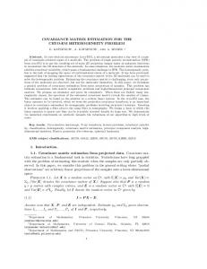
where xi = [xi,1 xi,2 ... xi,N ]T , si = T [si,1 si,2 ... si,N ] and zi = [zi,1 zi,2 ... zi,N ]T ∀i = 1, 2...L. Under the assumption of having white Gaussian noise components, zi is expressed as zi ∼ NL (0, σz2 IL ) where Nk (µ, σ 2 ) denotes k i.i.d. Gaussian random variable having a mean of µ and a standard deviation of σ, σz2 is the noise variance and IL is the identity matrix of order L. Suppose there is a b portion out of the whole B observation bandwidth that is occupied by a signal. In the received sample covariance matrix eigenvalues domain, M ≤ L tells that there is (M/L) fraction out of the whole observation bandwidth components which represent a transmitted signal and the rest ((L − M )/L) is noise only components. Accordingly, it can be stated that M/L = b/B . Fig. 1 illustrates the frequency domain received signal components model. When N, L → ∞ then the noise statistical covariance matrix Rz is defined as n o Rz = E z(n)zH (n) = σz2 IL , −∞ ≤ n ≤ ∞

(4)

−108

−110

Signal + Noise Componenets

−112

−114

dB

Noise Componenets

Noise eigenvalues

Signal + noise eigenvalues

−116

−118

b −120

B −122 0

5

10

15

20

Eigenvalue index

Fig. 1: Illustration of the received signal components in the frequency domain. where (.)H denotes the complex conjugate transpose. Similarly, the statistical covariance matrices of X and S which are denoted as Rx and Rs respectively, can be obtained using n o Rx = E x(n)xH (n) , (5) n o Rs = E s(n)sH (n) .

(6)

Rx = Rs + Rz = Rs + σz2 I.

(7)

Since the signal and the noise are independent, then

Assuming that Rx has the descendingly ordered eigenvalues λx1 , λx2 , ...λxL . In the same way, Rs has the descendingly ordered eigenvalues λs1 , λs2 , ...λsM . From (7), it can be found that λxi = λsi + σz2 ∀i = 1, 2, ..., M and λxi = σz2 ∀i = M + 1, M + 2, ..., L. ˆ x can be computed As in [9] sample covariance matrices, R instead of the statistical covariance matrices as there exists a finite number of samples. The sample covariance matrix of the received signal is calculated as ˆ x = 1 XXH . (8) R N While the statistical covariance matrix eigenvalues are equal to the signal components power, the sample covariance matrix eigenvalues are deviated from the signal power components and they follow Mar˘cenko Pastuer density [13] which depends solely on the value of (L/N ) refereed to as c throughout the rest of this paper. Mar˘cenko Pastuer density is explained in the next part of this section. Fig. 2 is a demonstrating example showing how the eigenvalues of both statistical and sample covariance matrices are located. Suppose a random sample covariance matrix having k eigenvalues where k → ∞, the distribution of those k eigenvalues converges to a non-random distribution function [14]. For a received Gaussian matrix of size N × L, the distribution function of its sample covariance matrix eigenˆ values F Rz (ν) → F W (ν) almost surely when N and L → ∞ and L/N = c is shown in (9)

Fig. 2: The 20 eigenvalues of the statistical covariance matrix (blue rings) and the sample covariance matrix (red stars). The signal has 10 dB SNR and occupies half of the observation bandwidth.

The density function depicted in (9) is called Mar˘cenko Pastuer density function which is introduced in [15]. Hereafter, the Mar˘cenko Pastuer density of parameters c and σz will be denoted as MP(c, σz ). Fig. 3a shows Mar˘cenko Pastuer density for different values of c while Fig. 3b shows both Marˇcenko Pastuer density and the empirical distribution for the sample covariance matrix eigenvalues for L = 1000 and c = 0.1. Both Fig 3a and Fig. 3b consider zero mean unitary variance Gaussian random signal. As shown in Fig. 3a, the higher the values of c the more is the spread of the sample covariance matrix eigenvalues around the Gaussian signal variance. Fig. 3b serves as a simulation verification of ˆ that F Rz (ν) → F W (ν) where F W (ν) is MP(c, σz2 ). III. T HE SNR E STIMATION A LGORITHM This section explains how to use the sample covariance matrix eigenvalues to estimate the received signal SNR. The process of the SNR estimation starts with determining the existence or absence of a signal. Consequently, if there is no signal the process stops and if a signal is detected then the samples covariance matrix eigenvalues are split into the noise and signal groups. Lastly, the SNR estimation algorithm explained in later in this section is applied. A. Binary hypothesis testing Before diving into how to estimate the SNR, we firstly need to determine whether there a signal exists or not. In other words, we need to perform the binary hypothesis testing for Ho and H1 described in (1). The binary hypothesis testing can be done using one of the spectrum sensing techniques surveyed in [16]. Since the SNR estimation algorithm considered in this paper is blind and eigenvalues based, then the maximumminimum eigenvalues detection (MME) [9] is considered for binary hypothesis testing. MME basically calculates the ratio between the maximum and the minimum eigenvalues of

12 c = 0.001 c = 0.01 c = 0.1 c = 0.5

1.4

8

dFW(ν)

e.d.f. Marcenko Pastuer density

1.2

dF (ν)/ Empirical dist.

10

6

W

4

1

0.8

0.6

0.4

2 0.2

0 0

0.5

1

1.5

2

2.5

0

3

0

0.5

1

1.5

ν

ν

(a)

(b)

2

2.5

3

Fig. 3: (a)Marˇcenko Pastuer density for different values of N and L. (b) Marˇcenko Pastuer density and the empirical distribution for 1000 eigenvalues at c = 0.1. dF

W

p √ √ (ν − σz2 (1 − c)2 ) (σz2 (1 + c)2 − ν) dν (ν) = 2πσz2 νc

(9)

where σz2 1 −

√
2 √
2 c ≤ ν ≤ σz2 1 + c .

!√ " √ "2 ! √ √ N+ L ( N + L)−2/3 −1 √ F1 (1 − pf a ) , 1+ Λ= √ (N × L)1/6 N− L  (λmax /λmin ) ≤ Λ H0 X→ Otherwise H1 .     1 θ(M ) ˆ + M (2L − M ) logN M = argmin −(L − M )N log φ(M ) 2 M where θ(M ) =

L Y

1/(L−M)

λi

and φ(M ) =

i=M+1

the signal sample covariance matrix and compare it with a threshold, Λ and declare either H0 or H1 accordingly. The maximum and minimum eigenvalues of the sample covariance matrix are denoted as λmax and λmin respectively; (10) and (11) summarises the essence of the MME. In (10) F1 is the cumulative distribution function of a Tracy-Widom distribution of order 1 since λmax has a Tracy-Widom distribution of order 1 [9]. pf a is the probability of false alarm defined as the probability of claiming a signal existence while noise only exists [17]. According to the value of (λmax /λmin ) the detector would make its decision as in (11). Even though the MME is integrated to the SNR algorithm introduced in this paper, it is yet not part of the algorithm and can be replaced by any other sensing technique. Not only that, but also the sensing part can be skipped and define a wall for the estimated SNR where values lower than this wall reflects a reception of noise only components.

1 L−M

L X

(10) (11) (12)

λi .

i=M+1

B. Estimating the SNR The sample covariance matrix eigenvalues based SNR estimator estimates the noise and the signal power individually and then use the property that the estimate of a ratio between two quantities is the ratio of those two estimated quantities [6]. As explained in Section II, the signal has M eigenvalues out of the whole L eigenvalues and the rest (L − M ) is the noise only eigenvalues. To estimate the value of M the ˆ is MDL criterion is used which estimates M as in (12). M ˆ the estimated value of M by the MDL. After determining M ˆ 2 the noise variance σz is estimated as follows. After obtaining  ˆ /L . Following that, the noise ˆ , βˆ is estimated as βˆ = M M representative eigenvalues located between λL and λMˆ +1 are 2 determined. Subsequently, two values of σz2 call them σz1 and 2 σz2 are found as

TABLE I: The SNR estimation algorithm. R&S SMU 100A vector signal generator

BEGIN - Calculate the sample covariance matrix Rˆx using (8). - Calculate the L eigenvalues of Rˆx . - Test H0 or H1 using 10 and (11). IF H1 - Estimate M using (12). - Estimate the noise and signal power using (15) and (16). - Estimate the γ using (17). ELSE BREAK END

PC running MATLAB (control and data collection) R&S FSQ 26 vector signal analysar

Fig. 4: The measuremets setup.

IV. E XPERIMENTAL AND R ESULTS

2 σz1 2 σz2

λL = √ 2, (1 − c) λMˆ +1 = √ 2. (1 + c)

(13a) (13b)

2 2 , σz2 ] are genK linearly spaced values in the range [σz1 erated and denoted as πk where 1 ≤ k ≤ K. After this ˆ step, K Marˇcenko Pastuer densities of parameters (1 − β)c 1 and πk where 1 ≤ k ≤ K are generated. Following that, the empirical distribution of the noise group eigenvalues is obtained and denoted as e.d. This noise eigenvalues e.d. is then compared with the K Marˇcenko Pastuer densities. The goodness of fitting is used to pick up the best πk as an estimate ˆz2 . The goodness of fitting for each πk , is denoted of σz2 , call it σ as D(πk ) which is defined as

 

ˆ πk D(πk ) = e.d. − MP (1 − β)c, (14)

, 2

where 1 ≤ k ≤ K and k.k2 denotes norm 2. The noise variance estimate is given by   (15) σ ˆz2 = argmin D(πk ) πk

After estimating the noise variance, the estimated signal power, Pˆs , is obtained by calculating the overall received power and subtracting the estimated noise power from it. (16) shows how the estimated signal power is fetched   L X N X 1 ˆz2 . Pˆs =  |xi,j |2  − σ (16) N L j=1 i=1 After estimating the signal and noise power, then the SNR is estimated as   L N P P 2 |x | i,j   Pˆs   j=1 i=1 (17) γˆ = 2 =  −1   σ ˆz N Lˆ σz2

where γˆ is the estimated SNR. Table I exhibits the algorithm of the sample covariance matrix eigenvalues based SNR estimation. 1 As

the signal occupies β portion of the observation bandwidth, then the noise occupies the rest (1 − β) of it

The evaluation of the performance of the described SNR estimation algorithm is performed via measurements. The measurements setup is depicted in Fig. 4. A WCDMA like signal is generated in a PC and directed to an R&S SMU 100A vector signal generator which is then forwarded to an R&S FSQ 26 spectrum analyser. The WCDMA like signal power is changed from −85 to −95 dBm with a step of 1dB. These values of the signal power are adjusted together with the spectrum analyser parameters to produce an SNR of approximately 0 to 10 dB. To evaluate the performance of the SNR estimation algorithm, a reference (actual) SNR is needed. The reference SNR is obtained by capturing the adjacent channel power ratio (ACPR) from the signal analyzer. The ACPR is the ratio between the power in the occupied channel and the adjacent channel which holds noise only components. The evaluation is divided into two parts, firstly, the performance of the algorithm in terms of the NMSE when the occupied and observation bandwidth are fixed and the values of N and L are changed, secondly, the changing of the occupied bandwidth inside a fixed observation bandwidth is studied. Every evaluation is based on 1000 measurements, 100 for each value of the signal power. A. The impact of N and L values at fixed occupied bandwidth For the evaluation of the influence of the N and L values, the occupied and observation bandwidths are fixed at 3 and 5 MHz respectively. These values of the occupied and observation bandwidths are arbitrary and picked up for testing the algorithm in the general case. Fig. 5 shows how the NMSE of the estimator is changed with the changing of N and L. It is observable from Fig. 5 that the NMSE of the estimator decreases with the increase of both N and L. The better performance with the increase of L is due to that the noise power will be extracted from higher number of the eigenvalues which gives better estimate. Moreover, the higher the value of N , the better realization of the signal and noise components is obtained. B. The influence of varying the occupied bandwidth Fig. 6 depicts the change of the SNR estimation NMSE when L and the occupation/observation bandwidth are changed. The curves in Fig 6 are obtained using a value of

−15

−20 N=1000 N=3000 N=5000

−25

L = 10 L = 20 L = 30 L = 40 L = 50

−20

−30

−35

NMSE [dB]

NMSE [dB]

−25

−40

−45

−30

−35

−40 −50

−45

−55

−60 10

15

20

25

30

35

40

45

50

L

Fig. 5: The obtained values for NMSE using different values of N and L.

2000 samples for N . As the figure illustrates, better estimation of the SNR is achievable with higher values of L and lower values of occupation/observation bandwidth. The change with L is explained in the previous subsection. The change with the occupation/observation bandwidth is explained as follows. As demonstrated in Section II, the ratio between the occupation and observation bandwidth, b/B determines the value of M estimated by the MDL. Subsequently, the noise variance is estimated from the smallest (L−M ) eigenvalues of the sample covariance matrix. Therefore, as it can be seen from Fig. 6, the smaller the occupied bandwidth, b, the smaller the value of M and the bigger the value of (L − M ). This makes the noise variance to be estimated from higher number of eigenvalues. Hence, for less occupation/observation bandwidth, the SNR is better estimated. V. C ONCLUSIONS An SNR estimation algorithm based on finite length sample covariance matrix eigenvalues is presented and evaluated in this paper. The estimator starts with the maximum-minimum eigenvalues detection. If a signal is detected, then the bandwidth occupied by that signal is estimated via minimum descriptive length criterion. The estimator performance is evaluated in terms of the normalized mean square error between the estimated and the reference SNRs. The reference SNRs are obtained using adjacent channel power ratios. The influence of changing the received vector size, the number of received vectors and the occupation/ observation bandwidth ratio is investigated. R EFERENCES [1] D. G. Brennan, “Linear diversity combining techniques,” Proc. of the IEEE, vol. 91, no. 2, pp. 331–356, 2003. [2] A. Svensson, “An introduction to adaptive qam modulation schemes for known and predicted channels,” Proc. of the IEEE, vol. 95, no. 12, pp. 2322–2336, 2007.

−50 0.1

0.2

0.3

0.4

0.5

0.6

0.7

0.8

0.9

Occupation/ observation BW (b/B)

Fig. 6: The NMSE values for different values of occupied/ observation bandwidth at different values of L. N is fixed at 2000 samples.

[3] D. Pauluzzi and N. Beaulieu, “A comparison of SNR estimation techniques for the AWGN channel,” IEEE Trans. Commun., vol. 48, no. 10, pp. 1681–1691, 2000. [4] B. Shah and S. Hinedi, “The split symbol moments SNR estimator in narrow-band channels,” IEEE Trans. Aerosp. Electron. Syst., vol. 26, no. 5, pp. 737–747, 1990. [5] R. B. Kerr, “On signal and noise level estimation in a coherent PCM channel,” IEEE Trans. Aerosp. Electron. Syst., vol. AES-2, no. 4, pp. 450–454, 1966. [6] R. Gagliardi and C. Thomas, “PCM data reliability monitoring through estimation of signal-to-noise ratio,” IEEE Trans. Commun. Technol., vol. 16, no. 3, pp. 479–486, 1968. [7] M. Rice, T. Oliphant, O. Haddadin, and W. McIntire, “Estimation techniques for GMSK using linear detectors in satellite communications,” IEEE Trans. Aerosp. Electron. Syst., vol. 43, no. 4, pp. 1484–1495, 2007. [8] T. Benedict and T. Soong, “The joint estimation of signal and noise from the sum envelope,” IEEE Trans. Inf. Theory, vol. 13, no. 3, pp. 447–454, 1967. [9] Y. Zeng and Y. C. Liang, “Eigenvalue-based spectrum sensing algorithms for cognitive radio,” IEEE Trans. Commun., vol. 57, no. 6, pp. 1784 – 1793, Jun. 2009. [10] M. Hamid, N. Bjorsell, W. Van Moer, K. Barbe, and S. Slimane, “Blind spectrum sensing for cognitive radios using discriminant analysis: A novel approach,” IEEE Trans. Instrum. Meas., vol. 62, no. 11, pp. 2912– 2921, 2013. [11] M. Hamid and N. Bjorsell, “Maximum minimum eigenvalues based spectrum scanner for cognitive radios,” in IEEE Int. Conf. on Instrumentation and Measurement Technology, May 2012, pp. 2248–2251. [12] M. Hamid, K. Barbe, N. Bjorsell, and W. Van Moer, “Spectrum sensing through spectrum discriminator and maximum minimum eigenvalue detector: A comparative study,” in IEEE Int. Conf. on Instrumentation and Measurement Technology, 2012, pp. 2252–2256. [13] R. Nadakuditi and A. Edelman, “Sample eigenvalue based detection of high-dimensional signals in white noise using relatively few samples,” IEEE Trans. Signal Process., vol. 56, no. 7, pp. 2625–2638, 2008. [14] A. Edelman and R. Nadakuditi, “Random matrix theory,” Acta Numerica., vol. 14, no. 7, pp. 233–297, 2005. [15] V. A. Marˇcenko and L. A. Pastur, “Distribution of eigenvalues for some sets of random matrices,” Math. of the USSR-Sbornik., vol. 1, no. 4, pp. 457–483, 1967. [16] T. Yucek and H. Arslan, “A survey of spectrum sensing algorithms for cognitive radio applications,” IEEE Commun. Surveys Tutorials, vol. 11, no. 1, pp. 116 –130, 2009. [17] W.-Y. Lee and I. Akyildiz, “Optimal spectrum sensing framework for cognitive radio networks,” IEEE Trans. Commun., vol. 7, no. 10, pp. 3845 –3857, Oct. 2008.