Alternative Hypothesis Tests for the Covariance Matrix Based on

Brazilian Journal of Operations & Production Management Volume 9, Number 1, 2012, pp. 9-27 http://dx.doi.org/10.4322/bjopm.2013.002

Alternative Hypothesis Tests for the Covariance Matrix Based on Eigenvalues and Multivariate Normality

Sueli Aparecida Mingoti Letícia Pereira Pinto Universidade Federal de Minas Gerais (UFMG), Belo Horizonte, MG

Abstract Three statistical tests for testing the covariance matrix in one population under multivariate normal assumption were developed and compared with the classical generalized variance test by means of Monte Carlo simulation. It is shown that the tests, which are based on the eigenvalues of the sample and the theoretical covariances matrices, presented better performance than the generalized variance particularly in cases which the parameters (determinant and traces) of the covariances matrices under the null and alternative hypothesis were similar. Since the three statistical tests are of simple implementation they can be considered as alternatives to be used in a general context.

Keywords: Generalized variance, Covariance matrix, Eigenvalues, Monte Carlo, Hotelling, Hayter and Tsui.

Introduction Hypothesis tests for the vector mean and the covariance matrix are very common when sampling from the multivariate normal distribution. Most of the papers better tests for the covariance matrix is also important. Practical examples appear in several areas particularly in quality control when the quality of the process is evaluated by measuring p characteristics simultaneously (p > 1). In this case location and variability parameters of the process have to be kept in certain pre-determined values in order to satisfy the established quality requisites (Montgomery, 2001). Some statistical tests have been proposed in the literature to test the covariance matrix (see Anderson, 1958; Costa and Machado, 2008; Yeh et al., 2006, for examples), however, the generalized variance, which is based on the determinant of the sample covariance matrix, |S|, is still very popular and it has been used also exact distribution of |S| under the null hypothesis is related to the distribution of the product of p independent random variables with chi-square distributions (Anderson, 1958; Aparisi et al.,1999). For simplicity, the normal distribution for |S| under the null hypothesis, is usually used as an approximation to construct the critical region of the test in practical situations. However, as shown by Djauhari (2009) the normal approximation for |S| just holds for large samples sizes. Another problem comes from the fact that

10 Brazilian Journal of Operations & Production Management Volume 9, Number 1, 2012, pp. 9-27

different matrices can present equal or similar determinants which contributes to the decreasing of the power of the generalized variance statistical test in detecting changes in the covariance matrix when they really take place. It is true that the determinant of the covariance matrix is equal to the product of its eigenvalues and that matrices with the same determinants not necessarily have similar eigenvalues structures (Timm, 2002). Therefore one possibility to improve the generalized variance test is to work with the eigenvalues of the covariance matrix instead of its determinant. In this paper three statistical tests will be developed by using this approach. Two of them are adaptations of the T2 Hotelling (1947) and the Hayter and Tsui (1994) statistical tests for population vector means and the third is based on the number of condition of the covariances matrices. The proposed tests will be compared to the generalized variance test by using Monte Carlo simulation. The power of the tests as well as the Average Run Length (Montgomery, 2001) will be estimated under several scenarios and different sample sizes. At the end of the paper an example of application

Generalized Variance Test Let X1, X2,...,Xn, where Xk = (Xk1, Xk2,...,Xkp)´, k=1,2,…,n, be a random sample of size n from a p-variate normal distribution with mean vector ´ and p covariance matrix , a pxp p is the number of random variables. Let Spxp 1

S pxp

n 1k

n

(Xk

X n )( X k

X n )´ 



1

where X n is the sample mean vector. Let the null and the alternative hypothesis be given as: H0: = 0 and H1: respectively, where 0 0 , 0 < < 1, the null hypothesis will be rejected for values of |S| < LCL or |S S| is the determinant of the sample covariance matrix.

LCL

b max 0, 0 1 z / 2 2 b1

, UCL

0 1

b z /2 2 b1

 

where

b1

1

p

( n 1 )p i 1

( n i ) ; b2

1

p

( n 1 )2 p i 1

p

(n i)

p

(n j 1

j 2)

(n j 1

j)



| 0| is the determinant of the 0 and z /2 is the value from the standard normal distribution which area above is /2. The test statistic (2) is based on the fact that under the null hypothesis E(|S|) = b1 | 0| and Var(|S|) = b2 | 0|2 (Montgomery, 2001). When the generalized variance test is used in quality control, for each sample of size n of the process the determinant of the sample covariance matrix as given in (1) is calculated. If the determinant |S| belongs to the critical region of the test the process is

11 Brazilian Journal of Operations & Production Management Volume 9, Number 1, 2012, pp. 9-27

declared as out-of-control. Usually, the values of |S| are plotted in a graph in sequential order of sample observations called control chart (Montgomery, 2001). The generalized variance is an interesting measure since it transforms a pxp matrix into a scalar number. However, it fails in many situations since different matrices can have equal determinants as next example shows. Example Consider the two matrices given in (3). Both matrices have determinants bivariate normal distribution with no correlation between the two random variables while in the second the correlation is equal 0.37. However, their eigenvalues structures are completely different since for 1 they are equal 1 and for 2 they are equal 2.404 and 0.4159, respectively. This fact raises the idea of constructing hypothesis tests based on the respective eigenvalues of the covariances matrices separatedly instead of in the determinant form. In the next section three new tests based on this concept will be presented. 1

1 0 and 0 1

2

2.32 0.4   0.4 0.5 



Statistical Tests Based on Eigenvalues In this section three statistical tests are presented. As described previously, for all tests it is assumed that X1, X2,...,Xn, where Xk = (Xk1, Xk2,..., Xkp)´, k=1,2,…,n, is a random sample of size n from a p-variate normal distribution with mean vector = ( 1, 2,..., p)´ and covariance matrix , a pxp p is the number of random variables. According to the spectral decomposition theorem (Timm, 2002) any covariance matrix pxpcan be expressed in terms of its eigenvalues i and the corresponding normalized eigenvectors ei, i=1,2,...,p, as given in (4) p pxp

i 1

i ei ei´

 

Let ˆ i , i = 1, 2,..., p, be the eigenvalues of the sample covariance matrix Spxp. When the random vector X has a p-variate normal distribution the eigenvalues ˆ i are asymptotically independent and for each i, ˆ i has a normal distribution with mean equal to the corresponding parameter i and variance 2 i2 / (n 1) (Timm, 2002). This result can be used in the construction of hypothesis tests for the covariance matrix as shown next. pxp

Hotelling T 2 Test Adapted for the Eigenvalues of the Covariance Matrix H1:

Let the null and the alternative hypothesis be given as H0: = 0 and , respectively. Let 0 = (1, 2,...,p)´, 1 , be the vector with the 0 p ˆ , ˆ ,..., ˆ ´ be the vector with , and ˆ 0

1

2

p

12 Brazilian Journal of Operations & Production Management Volume 9, Number 1, 2012, pp. 9-27

the eigenvalues of the sample covariance matrix Spxp, ˆ 1  ˆ 2  ...  ˆ p . The T 2statistic given in (5) is proposed to test the null hypothesis. T 2 (ˆ

1 0

0 )'

(ˆ

0)

p

(n 1)

i 1

2  2i

(

i

ˆ )2 i

 

where

2 12 / ( n 1) 0

0

...

0

2 22 / ( n 1) 0

0

0

0 0



0

0

2 2p / ( n 1 )

ˆ , ˆ ,..., ˆ ´ calculated considering = . is the covariance matrix of the vector ˆ 1 2 p 0 2 Under the null hypothesis T has approximately a chi-square distribution with p degrees 2 of freedom ( p ) , the null hypothesis will be rejected for observed values of T 2 larger than the critical value c, where P[ 2p c ] , 0 1.

The test statistic given in (5) is an adaptation of the Hotelling T 2 test statistic for the mean vector of one population (Hotelling, 1947). Due to the fact that the normal distribution of ˆ i is only asymptotic, the chi-square distribution of (5) is also an approximation. The exact joint distribution of the eigenvalues ˆ i can be found in Anderson (1958) but is complex. Due to these facts, in this paper the exact distribution of the test statistic given in (5) will be generated by Monte Carlo simulation and the performance of the test will be also evaluated under this situation. Hayter and Tsui Test Adapted for the Eigenvalues of the Covariance Matrix In 1994, Hayter and Tsui proposed a hypothesis test for the vector mean of one population. Its advantage to the Hotelling T 2 out automatically the variables whose means were different than the null hypothesis postulated values. However, as shown in Hayter and Tsui (1994) neither of the tests were uniformly more powerful. In this section we will present an adaptation of Hayter and Tsui´s test to the situation where the objective is to test the covariance matrix. M test statistic proposed by Hayter and Tsui (1994) and adapted in this paper for the eigenvalues takes the form given in (6).

M

max

 Yj , j

1,2,..., p

where

ˆ Yj

j

j



j 2 / ( n 1)







13 Brazilian Journal of Operations & Production Management Volume 9, Number 1, 2012, pp. 9-27

Due to the multivariate normality of the random vector X, the random variables Yj are independent and asymptotically normal. Therefore, under the null hypothesis the test statistic M is distributed as the maximum of the absolute values of p level , 0 < < 1, the null hypothesis is rejected for observed values of M larger than the constant called CR , such that P[M > CR, ] = . The CR value is obtained by using a simulation of samples from a p-variate normal distribution with zero mean vector and covariance matrix equal the correlation matrix (Ppxp) of the random vector ˆ ˆ , ˆ ,..., ˆ ´ which under the null hypothesis is the identity matrix. The basic 1 2 p steps of the simulation algorithm (see Hayter and Tsui, 1994) are given as follows: Step 1. Generate a large number N of vectors of observations from a p-variate normal distribution with zero mean vector and covariance matrix Ipxp.The generated vectors are denoted by Z1,Z2,...,ZN. Step 2. Calculate the statistic M for each of the generated vectors Zi Z1i , Z 2i ,..., Z ip ´ from step 1, i.e., for every i=1,2,…,N, calculate the value of the statistics Mi



max | Z ij |, j



1, 2,..., p 

Step 3. From the empirical distribution obtained from the sample (M1, M2,..., MN) as the critical constant C The values of Yj larger than CR identify the eigenvalues of the matrix

0

covariance matrix Spxp. Hypothesis Test based on the Number of Condition of the Covariance Matrix Another measure related to the structure of the covariance matrix is the number of condition which is used to evaluate the singularity of the matrix, i.e., to check if the matrix is badly conditioned or not. Generally speaking, the number of condition  ( A) = ||A||.||inv (A of a matrix A inv(.) the inverse matrix. When the quadratic norm is chosen and the matrix A is equal its transpose (A = A´), the number of condition of A is the ratio between its largest and its smallest eigenvalues as given in (7)

( A)

max min

 

The matrix A is considered badly conditioned if the number of condition is large. For some authors  ( A) > 20 is considered large enough (Greene, 1997). An interesting fact is that matrices with similar determinants may have different number of conditions. To illustrate this let´s consider again the matrices 1 and 2 given in (3). They both have determinants equal 1 but the number of conditions are different since ( 1) = 1 and ( 2) = 5.7788. Therefore, the number of condition can be used as an alternative to differentiate matrices with similar determinants but different components structures. Let H0: = 0 and H1: , be the null and the alternative hypothesis. 0 Let the test statistic (Spxp) be the number of condition of the sample covariance matrix

14 Brazilian Journal of Operations & Production Management Volume 9, Number 1, 2012, pp. 9-27

Spxp (Spxp) < c1 or (Spxp)>c2, where the constants c1 and c2 are obtained from the distribution of the test statistic (Spxp) under H0 and they are such that

PH0 [ ( S pxp ) c1 ] P[ ( S pxp ) c2 ]

, 0

1.

The distribution of the test statistic (.) under the null hypothesis is generated by Monte Carlo simulation and the critical region of the test is found according to the ) of the test. In this paper the constants c1 and c2 are such that

PH0 [ ( S pxp ) c1 ] P[ ( S pxp ) c2 ]

2

Comparing the Eigenvalues and the Generalized Variance Tests In this section the results of a Monte Carlo study are presented. A total of 10.000 random samples of sizes n = 5, 10, 25, 50 and 100 were generated from a multivariate normal distribution under the null (H0: = 0) and the alternative (H1: = 1 ) hypothesis being H0 tested for each sample and each test using 0.05 as 0 estimate of the probability of type I error of the test when data were generated under the null hypothesis and an estimate of the power of the test when data were generated under the alternative hypothesis. This procedure was repeated k=50 times under the null and the alternative hypothesis and at the end, average estimates of the probability of type I error and the power of the test were obtained by taking the average over all 50 repetitions for each test, respectively. For the generalized variance and the T2 eigenvalues tests the probability of type I error and the power were determined by using the asymptotic distribution of the test statistic as well as by the exact distribution obtained by Monte Carlo simulation through a generation of 50.000 random samples under the null hypothesis. Without loss of generality the study was performed considering one particular structure for matrix 0 for p = 2,3, assuming under H0 and H1. hypothesis test which presents the highest power values is the best. However, in the ARL (Average Length Run) value since in quality control samples of size n are observed average number of samples of size n taken until one indicates that the process is in the out-of-control condition (i.e. the value of the test statistic falls into the critical region of the test, or in other words, it falls outside the control limits). The ARL is given by the inverse of the probability (q) that the value of the test statistic falls in the critical region of the test, i.e., exceeds the control limits. When the process is under control q is the value of the probability of type I error and when the process is out-of- control q is the power of the test. Usually, when designing a control chart a small value of q, under control, is chosen such as 0.0027 for example, in order to decrease the rate of false alarms (a false alarm occurs when the process is declared out-of-control by the control chart when in fact it is not).Then, the test (or control chart) that detects faster

15 Brazilian Journal of Operations & Production Management Volume 9, Number 1, 2012, pp. 9-27

the true out-of-control situation of the process is preferred taking into consideration economical and operational issues also. For the study presented in this paper the value of q for the process under control is 0.05 which is not a value usually chosen to build a control chart. Independent of that, without loss of generality, the ARL out-of-control estimates of the tests were also estimated with the purpose of compared them on the light of the quality control point of view. Simulated Models The simulated models under the alternative hypothesis were chosen to make it possible to evaluate whether the statistical tests based on eigenvalues were able to detect small differences from 0 since it is already known that for larger samples and larger changes in 0 the generalized variance test has good performance. Tables 1 and 2 present the simulated models for p = 2 and p = 3 with the respective determinants, Table 1. Simulated models – p = 2. Cases

Covariance Matrices

null

2.32 0.40 0.40 0.50 

1

2.32 0.65 0.65 0.50  

0.7375

1

2

4

5

6

7

TR

ER

CR

5.7802

--

--

--

2.5280 2.82

8.6575

1.05 1

0.2920

2

1

0.42 1.41

1

2.32 0.30 0.30 0.50 

1.0700

2.32 0.50 0.50 0.75 

1.4900

7.1675

1.14 1.11

0.3820

5.2417

0.99 1

0.4518

4.0828

1.03 1.09

0.6040

2.32 0.57 3.32

3.2280

1.05 1.18

0.7850

4.32

2.2135

0.56 1.89

2.975 4.000

0.71 1.45

2.5340 1.9900

0.91 1.09

2.4660 3.07

1.24 0.92

2.3682 2.82

0.17 2.40

2.7380 3.12

1.5 0.7

1 1

1.0460

2.32 0.80 0.80 2.00

2

0.4159

2.32 0.90 0.90 0.80  

0.57 1.00 

,

1

2.4040 2.82

1 0 0 1

3

( )

1.24 1.53

1.344

0.38 3.23

TR , ER and CR: respectives ratios between the traces, eingenvalues and the number of conditions of the covariances matrices under H1 and H0; Case null denotes the covariance model under the null hypothesis;  between the two variables.

16 Brazilian Journal of Operations & Production Management Volume 9, Number 1, 2012, pp. 9-27

traces, eigenvalues and the number of conditions of the covariances matrices under H0 and H1. The ratios between traces, eigenvalues (only for p = 2), determinants and the number of conditions from the covariances matrices under H0 and H1 are also presented. For p = 2

but different 0 but with changes 0 in the variances; models 2 and 3 have different variances and correlations. For p = 3, except model 6. The covariances 0 but completely different 0 Table 2. Simulated models - p = 3 variables. Cases

Covariance matrices

null

1 0.6 0.6 0.6 1 0.8

( )

1

2

3

4

5

6

0.3 0.2 1 0.8 0.8 1 

1 0.3 0.2 0.3 1 0.8 0.2 0.8 1 

0.22

CR

11.69

0.46

-

-

-

1.00

1.00

1.38

1.50

1.00

0.86

1.64

1.00

0.77

3.32

1.00

0.24

2.27

1.00

0.34

9.73

2.00

0.95

1.76 0.22

16.09

1.13 0.11 1.93

0.33

10.02

0.87 0.19

0.36

1 0.3 0.3 0.3 1 0.4 0.3 0.4 1 

0.73

1 0.6 0.6 0.6 4 0.8 0.6 0.8 1 

TR

0.20

1 0.0 0.0 0.0 1 0.8 0.0 0.8 1 

1 0.5 0.5 0.5 1 0.5 0.5 0.5 1 

DR

2.34

0.6 0.8 1 

1 0.3 0.2

i,i = 1, 2, 3

1.80 9.00

1.00 0.20 1.67

2.78

0.73 0.60 2.00

0.50

4.00

0.50 0.50 4.36

2.14

11.10

1.25 0.39

DR, TR, and CR: respectives ratios between the determinants, traces and the number of conditions of the covariance matrices under H1 and H0; Case null denotes the covariance model under the null hypothesis.

17 Brazilian Journal of Operations & Production Management Volume 9, Number 1, 2012, pp. 9-27

covariances (correlations) structures and eigenvalues. The determinants of models 4, . An interesting case is model 6 0 , different 0 eigenvalues but similar number of conditions. The ratio of the determinants for the bivariate models, ranged from 0.7375 (case 1) to 4 (case 7). For the trivariate models the ratio ranged from 1 (case 1) to 9.73 (case 6).

Results and Discussion The averages proportion of rejection of H0 for each test discussed in this paper are shown in Tables 3 and 4, for p = 2, under the null and the alternative hypothesis models. The ratios (PR) between the estimated powers of the eigenvalues tests and the generalized variance test are presented in Table 5. When the exact distributions were used to build the critical region of the tests, the estimates of the probability of type I error were 0.05 as expected. However, for all sample sizes the estimates of the probability of type I error from the generalized variance test based on the normal distribution were it means that the amount of false alarms of the control chart will be larger than the expected under the null hypothesis. The difference was about 0.03 for n = 5, 0.02 for n = 10,25 and 0.01 for larger samples (n = 50, 100). This reinforces the fact that the normal approximation for the test statistic of the generalized variance test should be avoided for small samples and used with some care for samples sizes which are usually considered large such as n = 100. For n = 5, the estimate of the probability of type I error was also smaller than 0.05 for T 2 test when the chi-square distribution was used as a reference distribution to build the critical region of the test (estimate = 0.04). Due to these facts, in this study the comparison of the generalized variance with the three other statistical tests will be performed by considering the exact distribution only. For the T2 test both distributions (asymptotic and exact) will be used in the comparisons except for n = 5 for which only the exact will be considered. In general, the statistical tests based on the eigenvalues performed better than the generalized variance test considering the exact distribution (EGV) resulting in matrices 0 1 were very different (DR powers estimates of the generalized variance test were smaller than the values obtained for the T2(ET2) and Hayter and Tsui (HT) tests except for n = 5 where EGV presented similar performance than these two tests. For n ET2 and HT tests (see PR values in Table 5) over the EGV test in case 5 ranged from 18 to 46%; for case 6 from 6 (n = 100) to 40% (n = 25). For case 7 there was gain only for n = 10 (10 to 14%) being the EGV similar to ET2 and HT for the other samples in case 7 is 4 times larger 1 , a situation that favours the performance of the EGV test. 0 The condition number test (CN) presented smaller power estimates than EGV for cases 6 and 7 and more similar values for case 5. The generalized variance test presented very poor performance for cases 2, 3 and 4 since the power estimates were around 0.05 for all n. This can be explained although the matrices have 0 1 complete different correlation structures. Not even for n = 100 the EGV was able to

0.02

0.01

0.02

0.03

0.03

0.06

0.11

0.29

null

1

2

3

4

5

6

7

0.31

0.13

0.08

0.05

0.05

0.05

0.05

0.05

EGV

0.30

0.12

0.08

0.05

0.07

0.04

0.05

0.04

T2

0.32

0.14

0.09

0.05

0.08

0.05

0.05

0.05

ET2

0.30

0.13

0.08

0.05

0.07

0.05

0.05

0.05

HT

0.08

0.06

0.06

0.05

0.05

0.10

0.06

0.05

CN

0.60

0.23

0.12

0.04

0.04

0.03

0.01

0.03

GV

0.57

0.20

0.11

0.05

0.05

0.05

0.06

0.05

EGV

0.63

0.25

0.12

0.05

0.07

0.16

0.05

0.05

T2

0.65

0.27

0.13

0.06

0.08

0.17

0.05

0.05

ET2

0.64

0.26

0.13

0.05

0.07

0.17

0.04

0.05

HT

Average rejection of the null hypothesis n = 10

0.19

0.10

0.07

0.05

0.06

0.33

0.08

0.05

CN

0.94

0.48

0.22

0.05

0.05

0.03

0.01

0.03

GV

0.92

0.42

0.18

0.06

0.05

0.05

0.10

0.05

EGV

0.97

0.58

0.25

0.06

0.09

0.75

0.09

0.05

0.97

0.59

0.26

0.06

0.09

0.77

0.05

0.05

ET2

n = 25 T2

0.97

0.59

0.26

0.06

0.09

0.66

0.08

0.05

HT

0.72

0.40

0.21

0.11

0.14

0.97

0.25

0.05

CN

GV and EGV: the generalized variance tests with normal approximation and the exact distributions respectively; T2 and ET2: T2 Hotelling adapted for eigenvalues tests with chi-square and the exact distributions respectively; CN: condition number test. Case null denotes the covariance model under the null hypothesis.

GV

Case

n=5

Table 3. Probability of type I error and power estimates of the tests - p = 2, n = 5, 10, 25.

18 Brazilian Journal of Operations & Production Management Volume 9, Number 1, 2012, pp. 9-27

19 Brazilian Journal of Operations & Production Management Volume 9, Number 1, 2012, pp. 9-27

detect any difference between these two matrices (power estimate  0.07). For case 2 the power estimates of the ET2 and HT tests ranged from 0.05 (n = 5) to 1 (n = 50,100) being equal to 0.77 and 0.66 respectively for n = 25; the best test for case 2 however, was the CN (power estimates from 0.10 (n = 5) to 1 (n = 50,100) being equal 0.97 for n = 25. By Table 5 it can be seen that the power gains obtained by using CN instead of EGV for case 2 were very large (PR estimates ranged from 6.6 to 20). For case 3, although the power estimates of ET2, HT and CN tests were not very large, they were larger than the power estimates of the EGV for all sample sizes. The ratio (PR) between the estimated powers of these three tests compared to EGV ranged from 1.2 to 4.67 being CN the best test for this case (estimated powers between 0.05 to 0.28). the structure of the matrix 1 is very similar than the structure of 0, the estimated power values for all tests were low being CN the test more capable of detecting the difference between the two covariance matrices for n  25 (power estimates ranged from 0.11 to 0.14). In all cases, except for n = 5, the T 2 test using the chi-square distribution presented similar power estimates than T 2 with the exact distribution. This is an indication that for n the asymptotic distribution for the T 2 test statistic could be used instead of the exact distribution to build the critical region of the test. Under the practical point of view this is a good point in favour of using T 2 test regarding to its competitors HT and CN. It is important to point out that for n = 5 the majority of the power estimates of all tests were small (around 0.05 except for cases 6 and 7). This is due partially by the nature of the simulated models since some parameters of the 0 and 1 matrices Table 4. Probability of type I error and power estimates of the tests - p = 2, n = 50, 100. Average rejection of the null hypothesis n = 50 n = 100 T2 ET2 HT CN GV EGV T2 ET2

Case

GV

EGV

HT

CN

null

0.04

0.05

0.05

0.05

0.04

0.05

0.04

0.05

0.05

0.05

0.04

0.05

1

0.06

0.16

0.21

0.22

0.19

0.40

0.20

0.30

2

0.04

0.05

1.00

1.00

0.99

1.00

0.04

0.05

0.49

0.50

0.48

0.64

1.00

1.00

1.00

1.00

3

0.05

0.05

0.12

0.12

0.11

0.19

0.06

4

0.06

0.06

0.07

0.07

0.07

0.12

0.07

0.06

0.18

0.18

0.16

0.28

0.07

0.08

0.09

0.08

0.14

5

0.36

0.30

0.43

0.44

0.44

0.32

0.57

0.53

0.71

0.71

0.70

0.53

6

0.74

0.68

0.85

0.86

0.86

7

1.00

1.00

1.00

1.00

1.00

0.64

0.94

0.93

0.99

0.99

0.99

0.89

0.95

1.00

1.00

1.00

1.00

1.00

1.00

GV and EGV: the generalized variance tests with normal approximation and the exact distributions; T2 and ET2: T2 Hotelling adapted for eigenvalues tests with chi-square and the exact distributions; CN : condition number test. Case null denotes the covariance model under the null hypothesis.

1.00

0.68

0.99

4

5

6

1.12

1.30

1.18

1.00

1.40

3.40

0.67

1.03

0.84

1.13

2.60

2.33

6.80

ET2

0.97

0.68

1.00

2.40

2.11

5.80

HT

n = 10

1.14

1.35

1.18

1.20

1.60

3.40

0.83

0.07

0.95

1.06

0.50

0.55

1.20

CN

0.33

0.50

0.64

1.00

1.20

6.60

1.33

CN

1.00

1.34

1.30

3.53

3.71

17.20

T2

1.05

1.38

1.39

1.00

1.80

15.00

0.90

T2

1.05

1.40

1.44

1.00

1.80

13.20

0.80

1.00

1.39

1.32

3.63

3.86

17.60

ET2

0.99

1.34

1.27

3.53

3.71

15.80

HT

n = 25

1.05

1.40

1.44

1.00

1.80

15.40

1.00

n = 25 ET2 HT

0.05

1.29

1.26

0.42

0.43

2.40

CN

p=3

0.78

0.95

1.17

1.83

2.80

19.40

2.50

CN

p=2

1.00

1.37

1.07

2.85

3.61

20.00

T2

1.00

1.25

1.43

1.17

2.40

20.00

1.31

T2

1.00

1.26

1.46

1.17

2.20

19.80

1.19

1.00

1.37

1.08

2.88

3.65

20.00

ET2

1.00

1.37

1.07

2.85

3.61

20.00

HT

n = 50

1.00

1.26

1.46

1.16

2.40

20.00

1.37

n = 50 ET2 HT

T2 and ET2: T Hotelling adapted for eigenvalues tests with chi-square and the exact distributions respectively; CN: condition number test.

2

2.30

1.10

7

2.00

1.25

3

1.09

5

6

2

1.00

4

T2

1.40

3

6.00

3.20

2

1

0.83

1

Case

T2

Case

n = 10 ET2 HT

0.05

1.31

1.07

0.39

0.35

4.00

CN

0.95

0.94

1.07

2.00

3.80

20.00

2.50

CN

Table 5. Ratios (PR) between the estimated power of the eingenvalues and the generalized variance (EGV) tests.

1.00

1.09

1.00

1.82

2.53

20.00

T2

1.00

1.06

1.34

1.14

3.00

20.00

1.63

T2

1.00

1.06

1.32

1.14

2.67

20.00

1.60

1.00

1.09

1.00

1.82

2.54

20.00

ET2

1.00

1.09

1.00

1.82

2.54

20.00

HT

n = 100

1.00

1.06

1.34

1.29

3.00

20.00

1.67

n = 100 ET2 HT

CN

0.06

1.09

1.00

0.45

0.31

7.40

CN

1.00

0.96

1.00

2.00

4.67

20.00

2.13

20 Brazilian Journal of Operations & Production Management Volume 9, Number 1, 2012, pp. 9-27

21 Brazilian Journal of Operations & Production Management Volume 9, Number 1, 2012, pp. 9-27

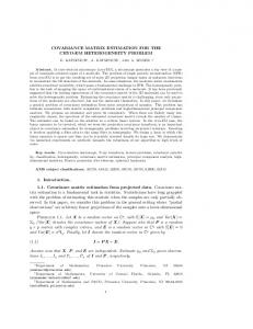
were very similar, and also by the sample size which statistically speaking, is too small to estimate the population covariance matrix properly. Table 6 presents the averages of the estimated proportions of rejection of H0 for each test, for p = 3. Only the results from sample sizes n 10 were considered since the proper estimation of the covariance matrix when p = 3 requires n larger than 6. The ratios (PR) between the estimated powers of the eigenvalues tests and the generalized variance test are presented in Table 5. When the exact distributions were used to build the critical region of the tests the estimates of the type I error were 0.05 as expected. Similar as seen for p = 2, the probability of type I error estimates for the generalized variance test with the normal distribution (GV) were smaller than 0.05 even for n = 50 (value around 0.03) being equal 0.04 only for n = 100. For these two respective sample sizes the GV estimates for all cases were very similar to the values of the exact test EGV. Due to these facts the results from GV will not be shown in the tables used as a support for the discussion presented in this section. The results from Table 6 show that the statistical tests T 2 and HT based on eigenvalues presented larger power estimates than the generalized variance test (except for case 5, n = 10, where they were similar) in some of the cases and they were able to detect the differences from 0 to 1 even for case 1, which the determinants of both matrices are equal. For this particular case the EGV test failed in detecting the differences even for larger samples sizes (estimated power = 0.05; n = 100) whereas the other two tests presented power estimates around 0.30 (for n = 10) and 1 (for n  25). The performance of the EGV test improved in cases 4, 5 and 6, resulting in similar values than T 2 and HT for case 6 which was expected since the determinant of 1 is 9.73 larger than the respective value of 0. For case 4 the EGV test also presented similar performance than HT for n = 10 but lower power estimates for n  25. By Table 5 it can be seen that for n 10 the gains in the power of the test by using the T 2 and HT were large for cases 1,2 and 3 ( PR ranged from for cases 1.82 to 20). For cases 4 and 5 the PR ratio ranged from 1.09 to 1.39 (for n 25) being around 1 for n = 10 and close to 1 for case 6. The number of condition test (CN) performs better than EGV for cases 1, 4 and 5 particularly for case 1 (PR ranged from 1.2 to 7.4) although the power estimates were not very expressive for this case (ranged from 0.06 to 0.37). For cases 2, 3 and 6 the CN test power estimates were lower than EGV specially for case 6 (estimated power around 0.05 for all sample sizes) which can be explained by the high similarity of the number of condition of both matrices 0 and 1. For p = 3, the T2 test based on the chi-square distribution (T2) had similar performance than the T2 based on the exact distribution (EGV). The ARL estimates out-of-control are shown in Figure 1 (for p = 2) and Figure 2 (for p = 3). The results indicated that the tests based on the eigenvalues could majority of the cases discussed in this paper these tests presented ARL values similar or lower than EGV, i.e., they were able to identify the true out-of-control condition faster than EGV even for smaller samples sizes and situations where the differences between the covariance matrices under the null and the alternative hypothesis were not very large.

0.05

0.05

0.09

0.10

0.32

0.19

0.75

null

1

2

3

4

5

6

0.74

0.13

0.32

0.23

0.18

0.30

0.04

T2

0.77

0.16

0.36

0.26

0.21

0.34

0.05

0.73

0.13

0.32

0.24

0.19

0.29

0.04

HT

0.05

0.18

0.34

0.05

0.05

0.06

0.05

CN

0.99

0.41

0.69

0.19

0.14

0.05

0.05

EGV

0.99

0.55

0.90

0.67

0.52

0.86

0.05

0,99

0.57

0.91

0.69

0.54

0.88

0.05

0.98

0.55

0.88

0.67

0.52

0.79

0.04

0.05

0.53

0.87

0.08

0.06

0.12

0.05

1.00

0.68

0.93

0.33

0.23

0.05

0.05

1.00

0.93

1.00

0.94

0.83

1.00

0.05

1.00

0.93

1.00

0.95

0.84

1.00

0.05

Average rejection of the null hypothesis n = 25 n = 50 T2 ET2 HT CN EGV T2 ET2

1.00

0.93

1.00

0.94

0.83

1.00

0.05

HT

0.05

0.89

1.00

0.13

0.08

0.20

0.05

CN

1.00

0.92

1.00

0.55

0.39

0.05

0.05

EGV

1.00

1.00

1.00

1.00

0.99

1.00

0.05

T2

1.00

1.00

1.00

1.00

0.99

1.00

0.05

1.00

1.00

1.00

1.00

0.99

1.00

0.05

n = 100 ET2 HT

CN

0.06

1.00

1.00

0.25

0.12

0.37

0.05

EGV: the generalized variance test with the exact distribution; T2 and ET2: T2 Hotelling adapted for eigenvalues tests with chi-square and the exact distributions respectively; CN: condition number test. Case null denotes the covariance model under the null hypothesis.

EGV

Case

n = 10 ET2

Table 6. Probability of type I error and power estimates of the tests - p = 3, n = 10, 25,50,100.

22 Brazilian Journal of Operations & Production Management Volume 9, Number 1, 2012, pp. 9-27

23 Brazilian Journal of Operations & Production Management Volume 9, Number 1, 2012, pp. 9-27

Under the quality control point of view the T 2 test has some advantage on Hayter and Tsui since for n 10 the chi-square distribution may be used to build the critical region of the test instead of the exact distribution, on the contrary of Hayter and Tsui´s which requires a simulation procedure to determine the constant CR , for any sample size n. Therefore, in practice the T 2 test is more feasible and for this reason it would be more appropriated in the quality control area even considering that the simulation procedure necessary to determine the constant CR is very simple and computationally fast. Example of Application In Montgomery (2001) an example was presented which two quality characteristics, the tensile strength ((X X1) and the diameter ((X X2), were measure in k = 20 samples of n Montgomery had established the following vector 0 and the matrix 0 as the parameters of the process in the under control condition:

0

115.59, 1.06 '

0

1.23 0.79 0.79 0.83 

Figure 1. ARL out-of-control estimates – n = 10,25,50,100 – p = 2.

24 Brazilian Journal of Operations & Production Management Volume 9, Number 1, 2012, pp. 9-27

Figure 2. ARL out-of-control estimates – n = 10,25,50,100 – p = 3.

The determinant of 0 is equal 0.3968, the eigenvalues are 1 = 1.8449 and 2 = 0.2151, the trace is 2.06 and the number of condition is 8.5769. The correlation between X1 and X2 is equal 0.782. To illustrate the statistical tests discussed in this paper 5 samples of size n = 10 were generated from a multivariate normal distribution with mean vector 0 being causes in the process which affected: (i) the standard deviation of the diameter of the the correlation between variables (sample 3); (iii) the standard deviations of both correlation between variables (sample 4); (iv) the standard deviations of both variables between variables (sample 5). The respective sample covariances matrices are given by

S1 S4

1.13 0.87 S2 0.87 1.04  2.80 2.69 S5  2.69 3.00 

1.28 0.95 S3 0.95 1.81 6.21 0.52 0.52 5.17 

4.26 0.25  0.25 0.73

25 Brazilian Journal of Operations & Production Management Volume 9, Number 1, 2012, pp. 9-27

Table 7. Example – Observed values of the tests statistics - p = 2 - n = 10. Sample 1

Sample 2

Sample 3

Sample 4

Sample 5

r12 = 0.80

r12 = 0.62

r12 = 0.14

r12 = 0.93

r12 = 0.09

Test EGV

0.418

1.414

3.047

1.163

31.835

T2

0.016

12.111

31.882

18.566

2212.97

ET2

0.016

12.111

31.882

18.566

2212.97

HT

0.127

3.389

4.905

4.308

46.746

CN

9.149

4.530

6.004

26.866

1.297

Rejection Regions: EGV 1.802; T2>11.829; HT>3.209; CN < 1.387 or > 108.119. r12: sample correlation between variables; 0.0027.

The corresponding eigenvalues ( ˆ 1, ˆ 2 ) of the sample covariances matrices are: 1.9562 and 0.2138 (sample 1); 2.5313 and 0.5587 (sample 2); 4.2776 and 0.7124 (sample 3); 5.5919 and 0.2081 (sample 4); 6.4254 and 4.9546 (sample 5). For each sample the null hypothesis H0

, was tested against H1

0

0

exact distribution and the tests based on the eigenvalues discussed in this paper. The results are given in Table 7 with the corresponding rejection limits for H0. Under the ˆ 1, ˆ 2 ) are given respectively by 0.8697 and 0.1014. All tests did not reject the null hypothesis for sample 1 and rejected for sample 5. This was expected since sample 1 came from a process under control and sample 5 came from a process with large variation in both variables affecting the covariance matrix strongly (the determinant of the sample covariance matrix S5 is ). The condition number (CN) failed in rejecting the null 0 hypothesis in samples 2,3 and 4 whereas the generalized variance failed in samples 2 and 4. On the contrary, Hayter and Tsui and T2 (with the exact and asymptotic distributions) statistical tests were able to detect all the changes performed in the parameters of the process since they rejected the null hypothesis for samples 2 to 5. Therefore, they were more appropriated than EGV and CN tests in this example.

Final Remarks The results presented in this paper showed that the adaptation of T2 Hotelling and Hayter and Tsui statistical tests based on the eigenvalues of the covariances matrices were more powerful than the generalized variance test, except for larger changes in the ), cases in 0 which the tests presented similar power estimates. It is important to point out that the T2 Hotelling and Hayter and Tsui statistical tests were able to detect small changes in , on the contrary of the generalized variance test. The test based 0 on the number of condition (CN and 0 had different eigenvalues structures but similar number of conditions. 1 Considering the results from the simulation study the T2 Hotelling and Hayter and Tsui statistical tests are better alternatives than the generalized variance test for the

26 Brazilian Journal of Operations & Production Management Volume 9, Number 1, 2012, pp. 9-27

covariance matrix under multivariate normal distribution, since they presented similar or larger power than the respective test. In terms of quality control Hotelling T2 test has some advantage since for n 10 it can be implemented by using the chi-square as a reference distribution to build the critical region of the test while Hayter and Tsui the simulation required for Hayter and Tsui simpler than the simulation required for the number of condition test.

Acknowledgments The authors were partially supported by the Brazilian institutions: CAPES-High Level Staff Improvement Coordination and CNPq- National Council

References Alt, F. (1985) Multivariate Quality Control, in: Kotz, S. and Johnson, NL. (Eds), Encyclopedia of Statistical Sciences. New York: John Wiley, pp. 110-122. Anderson, T.W. (1958) An Introduction to Multivariate Statistical Analysis. New York: John Wiley. Aparisi, F.; Jabaioyes, J. and Carrion, A. (1999) Statistical Properties of the |s| Multivariate Control Chart. Communication in Statistics - Theory and Methods, Vol. 28, No. 11, pp. 2671-2686. Costa A.F.B. and Machado, M.A.G. (2008) A New Multivariate Control Chart for Monitoring the Covariance Matrix of Bivariate Processes. Communication in Statistics - Simulation and Computation, Vol. 37, No. 7, pp. 1453-1465. Djauhari, M.A. (2009) Asymptotic Distribution of Sample Covariance Determinant. Matematika, Vol. 25, No. 1, pp. 79-85. Garcia-Diaz, J.C. (2007) The Effective Variance Control Chart for Monitoring the Dispersion Process with Missing Data. European Journal of Industrial Engineering, Vol. 1, No. 1, pp. 40-55. http://dx.doi.org/10.1504/EJIE.2007.012653 Greene, W.H. (1997) Econometric Analysis. Upper Saddle River: Prentice Hall. Quality Control Problems. Journal of Quality Technology, Vol. 26, No. 3, pp. 197-208. Hotelling, H. (1947) Multivariate Quality Control, in: Eisenhart, M.; Hastay, W. and Wallis, A. (Eds.), Techniques of Statistical Analysis. New York: MacGraw-Hill, pp. 111-184. Montgomery, D.C. (2001) Introduction to Statistical Quality Control. New York: John Wiley. Timm, N.H. (2002) Applied Multivariate Analysis. New York: Spring Verlag. Yeh, A.B.; Lin, D.K.J. and McGrath, R.N. (2006) Multivariate Control Charts for Monitoring Covariance Matrix: A Review. Quality Technology et. Quantatitative Management, Vol. 3, No. 4, pp. 415-436.

Biography Sueli Aparecida Mingoti is an Associate Professor at the Statistics Departament of Federal University of Minas Gerais (UFMG) located at Minas Gerais, Contact: [email protected]

27 Brazilian Journal of Operations & Production Management Volume 9, Number 1, 2012, pp. 9-27

Letícia Pereira Pinto is doctor student at the Statistics Department of Federal Spatial Statistics. Contact: [email protected]

Article Info Received: February, 2012 Accepted: June, 2012