cyber-physical systems with partly unknown software com- ponents. ..... Special care is taken if the .... such as automated lawn mowers or skid-steer loaders.
Sandboxing Controllers for Cyber-Physical Systems †
Stanley Bak† , Karthik Manamcheri† , Sayan Mitra† , and Marco Caccamo† University of Illinois at Urbana-Champaign, USA, {sbak2, manamch1, mitras, mcaccamo}@illinois.edu
Abstract—Cyber-physical systems bridge the gap between cyber components, typically written in software, and the physical world. Software written with traditional development practices, however, likely contains bugs or unintended interactions among components, which can result in uncontrolled and possibly disastrous physical-world interactions. Complete verification of cyber-physical systems, however, is often impractical due to outsourced development of software, cost, software created without formal models, or excessively large or complex models where the verification process becomes intractable. Rather than mandating complete modeling and verification, we advocate sandboxing of unverified cyber-physical system controllers by augmenting the system with a verified safety wrapper that can take control of the plant in order to avoid violations of formal safety properties. The focus of this work is an automatic method, based on reachability and time-bounded reachability of hybrid systems, to generate verified sandboxes. The method is shown to be both more general than previous work, and allows the trade-off of increased computation time for improved reachability accuracy. We also present an end-to-end toolkit which performs the low-level computation to generate the sandbox source code from Simulink/Stateflow models of a cyberphysical system.
I. I NTRODUCTION This paper addresses the problem of verifying properties of cyber-physical systems with partly unknown software components. Consider, for example, a firm A which manufactures autonomous vehicles outsourcing the development of the embedded controller to firm B. A provides to B a set of specifications, such as the details of the available sensoractuator signals, certain performance criteria, etc., based on which B then designs the controller and hands it back to A. In doing so, B may wish to provide the controller as a black-box without revealing the source-code or the core algorithms used for implementing it. How does A then guarantee the key safety properties of the autonomous vehicle that it manufactures without having complete access to B’s controller model? In an analogous situation, the controller model provided by B may be untrusted, or it may be too complicated to be analyzed in conjunction with the rest of the autonomous vehicle. As a more concrete example, consider the off-road vehicle industry, where vehicles traditionally made with hydraulics are starting to be built using steer-by-wire and drive-by-wire control. Software-based controllers may implement advanced features, such as locking the inner wheels on a sharp turn, to improve operator productivity. However, the unverified software may run on an unverified operating system which communicates to the actuators over a non-real-time network shared with other untrusted nodes. Complete verification is prohibitively expensive, yet an uncontained fault in the system
Fig. 1. The Simplex Architecture includes the physical plant, and three cyber components: a verified safety controller, a verified decision module, and an unverified complex controller.
could result in arbitrary actuation of both the steering and acceleration while the vehicle is in motion. Sandboxing is a popular technique for addressing these issues in the context of software and web-based security [1]. A sandbox is a testing environment that isolates untested and untrusted code and protects critical resources, such as live servers and their data, from changes that could be damaging. In this paper we present a technique for sandboxing controller software for cyber-physical systems in order to maintain formal safety invariants and, furthermore, automate the most difficult steps in the sandboxing process. Our sandboxing technique uses the Simplex architecture [2]. As shown in Figure 1, Simplex, given a complex, untrusted or unverified controller (CC), creates a protected environment for the plant by adding a safety controller (SC) and a decision module (DM) such that the DM activates the SC and deactivates the CC whenever the CC may jeopardize the safety of the system. The key challenge in using the Simplex approach is determining the switching conditions for the DM, that is, the states of the system in which it is safe to allow the CC to remain active and the states in which SC must take control in order to maintain safety, without being excessively conservative. Previously, Lyapunov-function-based techniques have been used to determine switching conditions for purely continuous systems [2]. Alternatively, for discrete systems, model checking can be effective for creating and verifying the switching logic [3]. For combined continuous and discrete systems, hybrid systems, we introduced an algorithm [4] which computes the switching set by performing reach-set computations on certain classes of hybrid automata. At a high level, our earlier approach [4] computes the switching set as follows: Let U be the set of unsafe states. No SC with bounded actuation strength can guarantee safety
from every state outside of U , U c . If the system is at the boundary of U then, because of delays and inertia, SC may not be able to prevent entry into U . Instead, we strive to find a smaller set R ( U c from which SC is guaranteed to drive the system in a way which avoids U . Formally, R is computed as the backwards reachable set, or backreach set, from U using the SC behavior and plant dynamics. Furthermore, the switching from CC to SC is not instantaneous as the DM can only observe the plant state and make decisions at most once every δ time, for some positive time interval δ. Thus, a still smaller set R0 ( R is computed where CC can be active for δ-time without threatening safety of the system. Once outside R0 , SC must be activated or safety may be violated. Formally, R0 is computed as the δ-time-bounded backreach set from R with the CC behavior and plant dynamics. Computing exact reach sets for hybrid systems is, in general, an undecidable problem [5], but various restrictive subclasses have been identified for which it is decidable [5], [6], [7]. The applications we have in mind cannot be modeled naturally using these decidable classes, and hence, we resort to overapproximating the reach sets. In our earlier approach [4], the backreach sets R and R0 were over-approximated by first creating discrete abstractions (simulations) of the system models, and then computing the backreach set and timebounded backreach set from the abstractions. One advantage of the algorithm was that it could be used for systems with some nonlinear dynamics. The earlier approach was used to guide the design and verification of the DM for a Simplex-based off-road vehicle system in order to prevent vehicle rollover. Although the algorithm from our previous work was a good first approach, several disadvantages were present. First, the models for which a discrete abstraction could be constructed were restricted. Second, even when a safe overapproximation of the backreach set could be produced, it was often excessively pessimistic (for example, the overapproximation computed of backreach of U in the SC model would be the entire state space). Lastly, no technique was provided to reduce the pessimism in the backreach computation. In this paper, we address these core technical limitations of the earlier algorithm and integrate it within a software tool suite for sandboxing controllers for cyber-physical systems. Specifically, the key contributions of this paper are: •
A fixpoint algorithm for computing backreachabililty which is applicable for a more general class of hybrid systems. The algorithm can be used with nonlinear dynamics as long as a function is provided which bounds each variable’s derivative in a section of the state space.
•
Three accuracy-increasing strategies which can be used to decrease the pessimism of the backreach computation. These are shown to be effective with an example, and an error-bounding theorem is provided.
•
A Simulink/Stateflow-based toolkit for generating the switching set for a given plant, CC, and SC, which automates the sandboxing process. The toolkit is applied on a case study of a skid-steer system, which illustrates the steps involved in system modeling and switching-set generation.
The organization of this paper is as follows. First, in Section II, we briefly review background material relevant to the discussion of our work. Next, Section III presents our algorithm for computing backreachability and time-bounded backreachability. The text is accompanied by pseudocode and accuracyimproving strategies and an associated error-bounding theorem is provided. Finally, we discuss a Simulink/Stateflow-based toolkit which uses our algorithm to automatically generate the source code for the Simplex switching set in Section IV. This is presented in the context of case study of a skid-steer vehicle system with nonlinear dynamics. The paper finishes with related work in Section V and conclusions in Section VI. II. P RELIMINARIES In this section, a brief review is provided about the Simplex Architecture and hybrid systems. The Simplex Architecture enables verification of control systems where the controller cannot be modeled completely. This feature is particularly advantageous where the model of the complex controller is unavailable or untrusted, or where it is too complicated to be tractable by verification procedures. The key components of a Simplex system (Figure 1) are (a) an abstract model of the complex controller (CC), (b) a safety controller (SC) and (c) a decision module (DM). Once every δ-time, the DM observes the plant and makes a decision about which controller (SC or CC) to activate. Roughly, if there is a possibility of entering an unrecoverable state within the next δ interval, then DM activates SC. Once SC restores the plant to a state from which there is no possibility of violating safety in the next δ-interval, it reactivates CC. We model each controller/plant combination in the Simplex system as a hybrid automaton. A hybrid automaton is a combination of differential equations with a finite state machine, where the state of the system can evolve both continuously and discretely. The continuous evolution of a hybrid system typically models the evolution of the physical variables in the plant, while the discrete transitions typically model software behavior. Formally, a hybrid automaton (HA) H = (V, L, S, θ, D, T ) consists of: (1) a set V of variables which define the dimensions of the system, (2) a finite set L of locations and `0 ∈ L, the initial location, (3) a set S of continuous states and a non-empty subset θ ⊆ S of start states, (4) a set D ⊆ L × L of discrete transitions and (5) a set T of trajectories (or flows) for V which define the continuous behavior of the system in a given location. Each location ` ∈ L, has an invariant condition I` associated with it. I` should be satisfied for the system to be in the location `. Each discrete transition τ ∈ T has a guard condition gτ and a reset map Rτ associated with it. A hybrid automaton
can transition from `1 to `2 , through a transition τ1 , if and only if the following conditions are satisfied: (a) I`2 should be satisfied, and (b) gτ should be satisfied. The complete formalism of hybrid systems has been further described in earlier work [8], [9], [10]. Let U be the set of unsafe states of the plant model. BackReach(U, SC) is defined as the set of states from which U can be reached within the SC hybrid automaton. G = BackReach≤δ (BackReach(U, SC), CC) is the set of states from which BackReach(U, SC) can be reached in up to δ time within the CC hybrid automaton. Previously [4], we showed that if SC is activated when the plant state is first detected to be in G then the overall Simplex system remains safe. Therefore, in principle, if we can compute the backwards reachable set of states with respect to SC, and time-bounded backwards reachable sets with respect to CC, we can generate a DM that is correct by construction. Unfortunately, as discussed earlier, the problem of computing backwards reachable sets for hybrid systems has been well studied and is, in general, undecidable [5]. Furthermore, an accurate model for CC may not be available for the reasons presented in the introduction. We can circumvent these issues by computing an overapproximation G 0 ⊇ BackReach≤δ (BackReach(U, SC), CC ’) based on an abstract model CC0 of the complex controller. For example, the actual outputs generated by CC can be abstracted by the range of values that are valid outputs for the actuators. Since G 0 overapproximates G, using G 0 as the switching set also guarantees overall system safety.
v v max
x min
x max
x
v min Unrecoverable States (a) if (vmax )2 /(2 ∗ amin ) < xmax
v v max
x min
x max
x
v min Unrecoverable States (b) if (vmax )2 /(2 ∗ amin ) > xmax Fig. 2. The gray area indicates BackReach(U , SC), which are states where using the safety controller leads to safety violations for the example from Section III-A.
III. C OMPUTING BACKREACHABILITY In this section, we describe the details of the algorithm used to construct Simplex switching set by overapproximating the equation BackReach≤δ (BackReach(U, SC), CC ’). Throughout this section, we will augment the discussion with a demonstrative Simple-Vehicle System, which is introduced in Section III-A. Section III-B presents the assumptions of our backreachability algorithm. Next, Subsection III-C presents the algorithm for computing bounded and unbounded backreach sets. Finally, in Section III-D, three strategies are proposed which together can bound the error of a BackReach≤δ computation to an arbitrary constant. Additionally, although we are concerned with backreachability for Simplex, the explanations are easier to understand, and therefore presented, in terms of forward reachability. The two notions can be shown to be computationally equivalent. A. Simple-Vehicle System Example Consider a vehicle which moves along a one-dimensional line, modeled as a point x on the x-axis which moves according to the input acceleration a generated by the controller. Physical constraints require that a ∈ [amin , amax ], and the velocity of the vehicle remains in the range [vmin , vmax ]. The safety property requires that the point x remains in the range [xmin , xmax ], where xmin < 0 < xmax . For simplicity, we assume xmin = −xmax , vmin = −vmax and amin = −amax .
For this system, one possible safety controller is a bangbang controller which outputs the maximal negative acceleration a = amin for x > 0 and outputs a = amax if x ≤ 0. Two possible sets of unrecoverable states (depending on the exact parameters of the plant) are shown in Figure 2. This region can be computed directly by examining the backreachability using the SC automaton from set of unsafe states, U, or formally BackReach(U, SC). Next, we specify the hybrid automata for the CC ’ system and system, which are show in Figure 3. The hybrid automaton for the CC ’ system, in Figure 3(a), has three locations (discrete modes). Under unsaturated operation, the location invariant is vmin < v < vmax and the derivative equations are x˙ = v and v˙ = [amin , amax ] (v˙ is nondeterministic). There are two other locations corresponding to when the point has reached its minimum and maximum velocity (labeled min speed and max speed) where v˙ is restricted to be either nonnegative or nonpositive. The hybrid automaton for the SC, in Figure 3(b), contains two locations corresponding to the two states of the controller (labeled forward and backward), and two more locations for when the velocity has reached saturation (labeled min speed and max speed). When we compute an overapproximation of BackReach or BackReach≤δ , it will be with respect to one of these automata. SC
min_speed
unsaturated
v˙ = 5 x˙ = v
Invariant:
max_speed
v˙ = [5,−5] x˙ = v
v˙ = −5 x˙ = v
Invariant:
Invariant:
v min v v max
v = v min
(a) the CC ’ (complex controller abstraction and plant) automaton max_speed
min_speed
v˙ = 0 x˙ = v
v˙ = 0 x˙ = v
Invariant:
Invariant:
x≤0 ∧ v=v max
x0 ∧ v=v min
forward
backward
v˙ = 5 x˙ = v
v˙ = −5 x˙ = v
Invariant:
x≤0 ∧ vv max
x
v
x
v
v = v max
Invariant:
x0 ∧ vv min
(a) the CC ’ derivative dependency graph
Fig. 4. The derivative dependency graphs for the Simple-Vehicle System have explicit dependencies (solid arrows) and implicit dependencies (dashed arrows).
For the CC ’ automaton, dbmin = v lower , dbmax = v upper , x x � −5 if v upper > vmin dbmin = v 0 otherwise and dbmax v
(b) the SC (safety controller and plant) automaton Fig. 3. The hybrid automata describing the Simple-Vehicle System have no transition guard restrictions, so the discrete location switching is done solely based on the invariants.
B. System Assumption In order to apply our algorithm, we have two assumptions, which we outline and elaborate on in the context of the SimpleVehicle System below. Assumption 1: For any rectangular set of states H ⊆ S, for any continuous variable xi , there exist functions dbmin and xi dbmax , that bound the derivative of x with respect to time in i xi dxi max H. That is, dbmin (H) ≤ ≤ db (H), for every x . i xi xi dt Assumption 2: We make a distinction between two types of derivative dependencies, explicit ones directly extracted from the differential equations in each location of the hybrid automaton (for example, w˙ = v would create an directed edge from the node corresponding to v to the node corresponding to w), and implicit dependencies which arise because as time advances, the continuous state may cause a change in hybridautomaton locations which causes the differential equations of variables to be changed. Assumption 2 restricts the systems we consider to those where the explicit dependency graph of the state-variable derivatives does not have cycles, except for self-loops. This restriction is more relaxed than in our previous work, where the combined explicit / implicit derivative dependency graph was required to be acyclic, except for selfloops. Example: In the context of the Simple-Vehicle System, to meet Assumption 1, we must provide the derivative bounds functions for each variable, x and v, which can be automatically extracted from the hybrid automata. These functions takes as input a rectangle of the state space defined by upper and lower bounds on each variable, ([v lower , v upper ] × [xlower , xupper ]).
(b) the SC derivative dependency graph
� =
5 0
if v lower < vmax otherwise
= = v lower , dbmax For the CC ’ automaton, again, dbmin x x v , and upper upper −5 if xupper > 0 ∧ v upper > vmin 0 if x >0∧v ≤ vmin = dbmin upper upper v 0 if x ≤ 0 ∧ v ≥ vmax 5 otherwise upper
and dbmax v
5 0 = 0 −5
if xlower ≤ 0 ∧ v lower < vmax if xupper > 0 ∧ v upper ≤ vmin if xupper ≤ 0 ∧ v upper ≥ vmax otherwise
To meet Assumption 2, we construct and check the derivative dependency graphs (shown in Figure 4). For both controllers, in every location, the value of x, ˙ explicitly depends on v, and the value of v˙ does not explicitly depend on any variables. However, due to the possibility of a change in automaton location, there is an implicit dependence of v˙ on v in the CC ’ automaton. In the SC, there are two implicit dependencies: one implicit dependence of v˙ on v, and a second implicit dependence of v˙ on x. Since both of the explicit dependency graphs (solid arrows) with self-loops removed are acyclic, the system meets the second assumption. Notice, however, that the SC automaton would not meet the restrictions of our previous algorithm since the combined explicit / implicit derivative dependency graph contains a cycle that is not a selfloop. C. Algorithm for Overapproximating Reach and Reach≤δ In this section, we outline our proposed algorithm for computing overapproximations of Reach and Reach≤δ . We start by presenting the pseudocode of the algorithm, and then elaborate on each of the functions. The pseudocode uses the following notation: The expression D.i refers to the ith element of a finite set D in an arbitrary fixed ordering. The expression H/i refers to the projection of the ith dimension of a hyperrectangle H. The minimum
value in this one-dimensional projection is referred to by 34 min max H/i and the maximum value is referred to by H/i . The 35 36 hybrid automaton has n continuous variables, x1 , x2 , . . . , xn , 37 which are ordered according to the topological sort of the 38 39 explicit derivative dependency graph with self-loops removed. 40 The values qxi for each variable xi are quanta used in the 41 42 computation which are fixed constants. 43 44 In the pseudocode, several functions are also used: 45 • getLocations takes a hyperrectangle state space as 46 input and outputs a set of integers corresponding to the 47 48 set of locations in which the hybrid automaton may be. 49 50 • getFirstImplicitDerivativeDependency 51 takes as input an integer corresponding to an automaton 52 location, and returns the implicit derivative dependency 53 54 of the node corresponding to xi that comes first in the 55 56 topologically-sorted variable order. 57 • α is an abstraction function which takes as input a set 58 of states, and outputs a set of abstract states represented 59 60 an integer for each variable. The α−1 function is the 61 concretization function which, given an abstract state, 62 63 returns the set of corresponding concrete states of 64 the system. Formally, if the continuous state space 65 66 is X = Rn and the abstract state space is Y = Zn , then α : X −→ Y. α(x) = y1 , y2 , . . . , yn , where each yi = xi /qxi and xi refers to the ith coordinate of a state x ∈ X . In the abstraction function, qxi are the constant quanta for each variable, as mentioned above. As usual, α−1 : Y −→ 2X . In the pseudocode, we use the natural lifting of these functions from a single input state to a set of input states. The pseudocode for the reachability and time-bounded reachability algorithms is below: 1 2 3 4 5 6 7 8
%%% ComputeReach outputs an overapproximation of reachability from an initial set ComputeReach(I} { declare D := α(I); declare C := α−1 (D); declare m := |D|; % number of abstract states declare array[m] E; declare C 0 := ∅;
9
for i = 1 to m E[i] := α−1 (D.i); % initialize the m exact reach sets
10 11 12
while (C 6= C 0 ) % loop until fixpoint C 0 := C;
13 14 15
for (i = 1; i < m; i := i + 1) (H, E) := ComputeDeltaReach(E[i ]); E[i ] := E; % update exact reach set C := C ∪ H; % accumulate reachability
16 17 18 19 20
return C;
21 22
}
23 24 25 26 27 28
%%% ComputeDeltaReach outputs (Reach≤δ , Reachδ ) from an input hyperrectangle ComputeDeltaReach(H) { declare E := H; declare L := getLocations(H);
29 30 31 32 33
for (i = 1; i < n; i = i + 1) % loop over every variable declare l = MinReach(i, H); declare u = MaxReach(i, H);
E/i := [l, u]; % update exact delta reach max H/i := [min(Hmin , u)]; % update delta reach /i , l), max(H/i if (L 6= getLocations(H)) L := getLocations(H); i := getFirstImplicitDerivativeDependency(i) − 1; % backtrack return (H, E) } %%% MinReach overapproximates the minimum value of xi reached after δ time MinReach(i, H) { min return MinReachRecursive(H, i, δ, Hmin /i , dbxi , true); } %%% MinReachRecursive overapproximates the minimum value of xi reached MinReachRecursive(i, H, time, start, db, isFirstInterval) { H/i := [start −qxi , start ]; % consider the current interval declare der := db(H); declare nextIntervalTime := (der = 0 ? time : −qxi /der);
}
if (nextIntervalTime < 0) % switch direction if (!isFirstInterval) % can not safely reverse direction; be pessimistic return start; else return MaxReachRecursive(i, H, time, start, db, false); else if (nextIntervalTime ≥ time) % time expires in this interval return start + nextIntervalTime ∗ der; else % continue to next interval return MinReachRecursive(i, H, time − nextIntervalTime, start −qxi , db, false);
The top-level of the algorithm, the ComputeReach function (lines 1-22), starts by dividing the state space into hyperrectangles based on a provided constant quantum size for each variable through the abstaction function α (line 4). The fixpoint computation loop for computing reachability occurs on lines 13-19. Starting from the hyperrectangle corresponding to every discrete state which contains an unsafe state, we use the ComputeDeltaReach function to compute both the states reachable in up to δ time, Reach≤δ , and the states reachable in exactly δ time, Reach=δ (line 17). The Reach=δ result is used as the initial set of states for the next iteration of the loop (line 18), while the Reach≤δ result is added to the global reachable set (line 19). The intuition behind the correctness of this function is that any state reachable in up to k < δ time will necessarily pass through a state reachable in exactly δ time (specifically, after δ − k time). Therefore, we need not consider all of Reach≤δ as the initial states in the next iteration. In terms of termination, notice that this algorithm will clearly not terminate if the computed reach set is infinite. If termination is desired, one can bound the reachable state space with the hybrid automaton, and assure the the variable derivatives do not asymptotically approach 0 (for example, by adding an � amount of overapproximation in the dbmin and dbmax functions). xi xi The ComputeDeltaReach function (lines 24-42) is used to overapproximate both Reach≤δ and Reach=δ . Starting from an input initial hyperrectangle, the sets of states are computed for each variable in the order of the topological sort of the explicit derivative dependency graph with self-loops removed (lines 30-39). This ensures that when the bounds is being computed for a particular variable, all (non-self) dependent variables already have valid computed Reach≤δ bounds, ensuring correctness. After a Reach≤δ bound for a variable is
computed, this bound is used as input to the derivative bounds function that is used to compute Reach≤δ for the subsequent dependent variables (because of the assignment on line 35). The Reach=δ set is also maintained (line 34). After we have computed Reach≤δ for every variable, the cross product is an overapproximation of Reach≤δ from the initial state (which is iteratively constructed on line 35). The proposed algorithm does allow models with cycles caused by implicit derivative dependencies, restricting only that the explicit-only dependency graph of derivatives be acyclic except for self-loops. After we compute the Reach≤δ for a variable with an implicit derivative dependency which creates a cycle in the combined explicit / implicit derivative dependency graph, we go back and check if we may have entered a new state of the automaton (line 37). If we may have, the algorithm backtracks and recomputes the reachability of all the variables that could have possibly been affected (line 39). Since there are only a finite number of discrete locations in the hybrid automaton, the backtrack process can only happen a finite number of times, and the algorithm remains terminating. Example: Consider computing Reach≤δ in the SimpleVehicle System with respect to the safety controller / plant automaton (Figure 3(b)), starting from (x = [−2, −1], v = [4, 5]). We fix the quanta of both dimensions to be 1, fix δ to be 0.5 time units, fix vmax to be 10, and fix amin = −5 and amax = 5. The algorithm will compute in the order of the explicit dependency graph, first v then x. First the reachability for v is computed using MinReach and MaxReach. These two functions return 6.5 and 7.5, respectively. Due to the capping of the minimum value (line 35) the Reach≤δ range is set as v = [4, 7.5]. Second, the reachability for x is computed to be x = [−2, 2.75]. The algorithm can not terminate here, since the change in x may result in a change in hybridautomaton location (the condition on line 37 is true). The algorithm goes back and recomputes Reach≤δ for v to be v = [1.5, 7.5]. Next, the reachability of x is recomputed once again to be x = [−2, 2.75]. Although there is an implicit dependency, the set of possible discrete locations has not changed since the last iteration (the condition on line 37 is false due to the prior assignment on line 38), and the loop terminates. The result of the algorithm is an overapproximation of the actual Reach≤δ states, shown in Figure 5. The MinReach and MinReachRecursive functions (lines 44-66) (and symmetric MaxReach and MaxReachRecursive, not shown), overapproximate Reach=δ for one variable, under the assumption that the passed-in hyperrectangle contains valid Reach≤δ bounds for all dependent dimensions. This is done by starting at the minimum value of the variable in the initial hyperrectangle (line 47), and proceeding at the minimum derivative for δ time, considering new derivatives as we enter new intervals (line 53). Intuitively, this is correct because the all the bounds of the dependent dimensions is correct are assumption so the call to db (line 54) will yield a correct bound on the current variable’s derivative. If the derivative is nondeterministic, we will still overapproximate Reach=δ by considering
v
−2,5
−1,5
−2,4
−1,4
x Fig. 5. An estimate of Reach≤δ in the computed using 10,000 simulations (light gray region) for the Simple-Vehicle System is shown in comparison with the overapproximation computed with proposed Reach≤δ algorithm (solid gray line). This computation is done with respect to the SC automaton. Here, δ is 0.5 and the initial state is (x = [−2, −1], v = [4, 5]).
the minimum in each interval. Special care is taken if the derivative is zero (line 55), or if the minimum derivative is positive (lines 58-61), which avoids infinite loops caused by Zeno behavior through the isFirstInterval variable. Example: To help illustrate this algorithm, we compute Reach≤δ from a state in the Simple-Vehicle System, in the CC ’ automaton (Figure 3(a)). Now, we will compute Reach≤δ from the hyperrectangle (x = [1, 2], v = [8, 9]). The topological sort of the self-loop-removed derivative-dependency graph (Figure 4(a)) is v, x, so we start with the v dimension. The inner loop of the algorithm, MinReach and MaxReach, will compute the minimum and maximum values of v that can be reached after δ time. In the functions, the variable time is used to keep track of the time elapsed in terms of the execution of the system when computing these values. Initially, time = δ = 0.5. To compute the minimum reachable velocity, we start by invoking dbmin with the v hyperrectangle (x = [1, 2], v = [7, 8]), which outputs the derivative bounds -5. At the minimum derivative, -5, the next interval is reached in 0.2 time units. We update time to be 0.5 − 0.2 = 0.3. The process then repeats for the next interval, v = [6, 7]. The minimum derivative for v is again -5, and time is updated to 0.1. On the third iteration, time is less than the time it would take to reach the next interval, and the minimum Reach≤δ value is computed as v = 4.5 (line 63). To compute the maximum velocity we again, initialize time to be δ = 0.5. First, dbmax with the hyperrectangle v (x = [1, 2], v = [9, 10]) outputs 5 as the maximum derivative
v v max 1,9
2,9
1,8
2,8
Fig. 6. An estimate of Reach≤δ computed using 10,000 simulations (light gray region) for the Simple-Vehicle System is shown in comparison with the overapproximation computed with the proposed Reach≤δ algorithm (solid gray line). This computation is done with respect to the CC ’ automaton. Here, δ is 0.5 and the initial state is (x = [1, 2], v = [8, 9]).
for the v variable. The time variable is updated to 0.3. On with the hyperrectangle the second iteration, however, dbmax v (x = [1, 2], v = [10, 11]) outputs 0 as the maximum derivative for the v variable, so the next interval is unreachable in 0.3 time units. The maximum Reach=δ value is therefore v = 10 (line 63). The Reach=δ values for v are [5, 10] Now the ComputeDeltaReach function would proceed to compute the reachable values for the next variable, x, using the values [5, 10] for the v-dimension of the hyperrectangle when calling MinReach and MaxReach. Computing the maximum value that can be reached for x, the states of the computation proceed as: (x = [2, 3], v = [5, 10]) = 10); (t = 0.5, x = [2, 3], dbmax x (x = [3, 4], v = [5, 10]) = 10); (t = 0.4, x = [3, 4], dbmax x (x = [4, 5], v = [5, 10]) = 10); (t = 0.3, x = [4, 5], dbmax x (t = 0.2, x = [5, 6], dbmax (x = [5, 6], v = [5, 10]) = 10); x (t = 0.1, x = [6, 7], dbmax (x = [6, 7], v = [5, 10]) = 10). x where t is the value of time. At this point, the next interval can not be entered in 0.1 time, and the maximum Reach≤δ value is x = 7. Computing the minimum value x can reach, we start with t = 0.5 and invoke dbmin with the hyperrectangle (x = x [0, 1], v = [5, 10]). This returns a minimum derivative in the x dimension of 5, which is nonnegative, so we switch directions and call MaxReachRecursive (line 61), with the dbmin x function as a parameter. This will eventually reach a minimum Reach=δ value of x = 6. The Reach=δ values are x = [6, 7]. This example is shown in Figure 6. D. Accuracy Convergence One important concern for using the proposed algorithm to compute the Simplex switching set is the accuracy of the Reach≤δ overapproximation, which in turn affects the accuracy of the global-reachability overapproximation that it computes. In this subsection, we propose three strategies that can be used to reduce the error of the proposed algorithm. Then, an important accuracy theorem is stated which allows
us, under some reasonable assumptions, to reduce the computed Reach≤δ error for each variable to an arbitrarily small constant. Finally, through example, the proposed strategies are shown to, in fact, reduce the computed error. We propose three strategies to reduce the error of the Reach≤δ region from an initial hyper-rectangle, which we call the quantum rule, the refine rule and the split rule. We later show that these, when used in combination, can reduce the error in each variable of the Reach≤δ overapproximation to an arbitrary constant. The quantum rule uses the fact that the inner loop (MinReach and MaxReach) of the algorithm considers intervals one quantum in size. Since no restrictions are placed on the minimum size of the quantum, the quantum rule, which evenly splits the size of this quantum for one variable, is always safe to apply. Intuitively, this helps with accuracy by, at each time, providing a smaller hyperrectangle to the derivative bounds function which allows it to output a more accurate derivative bound. The refine rule is based on the fact that Reach≤δ from an initial set, w, is equal to the union of Reach≤δ from multiple smaller sets, as long as the union of those smaller sets is equal to the initial set w. Formally, if w = w1 ∪ w2 ∪ . . . ∪ wn , then Reach≤δ (w) = Reach≤δ (w1 ) ∪ Reach≤δ (w2 ) ∪ . . . ∪ Reach≤δ (wn ). This allows us to refine the initial hyperrectangle into smaller hyperrectangles and still obtain a safe overapproximation by taking the union of the results. The rule itself will be applied to a particular variable, and will split the initial hyperrectangle into equal-sized hyperrectangles along that variable. As with the quantum rule, this intuitively helps with accuracy by providing a smaller hyperrectangle to the derivative bounds function which allows it to output a more accurate derivative bound. The final rule, the split rule, is based on the fact that Reach≤δ can be decomposed in a way similar to the way in which we described computing full reachability the ComputeReach function. Formally, d1 + d2 + . . . + dn = δ implies that Reach≤δ (w) = Reach≤d1 (w) ∪ Reach≤d2 (Reach=d1 (w))∪ Reach≤d3 (Reach=d2 (Reach=d1 (w))) ∪ . . .. When we say this rule is applied n times, we split δ with n equal constants, d1 = d2 = . . . = dn = nδ . Intuitively, this rule will improve accuracy by, when computing the reachability for a particular variable, reducing the variable ranges of the dependent dimensions. This provides the derivative bounds function with a smaller hyperrectangle, which allows it to output a more accurate derivative bound. The application of these three rules can be used to reduce the pessimism of the error in the Reach≤δ overapproximation in each discrete mode to an arbitrarily small constant in each dimension. This is reflected in the following statement: Claim 1: By applying the quantum rule, the refine rule and the split rule finitely many times, the maximum error in each variable x of the computed Reach≤δ overapproximation in a single mode, for a fixed δ and from an initial hyperrectangle α, can be reduced to below an arbitrary positive constant ex .
v
v
The controller software periodically senses the position (x, y), the velocity v, and the heading θ, of the vehicle and ˙ based on the sets the acceleration (v) ˙ and the steering (θ) ∗ ∗ current waypoint (x , y ) of the system. The vehicle models a skid-steer system which can turn in place, i.e., the heading θ can change even when the velocity v is 0. The equations of motion for the vehicle’s position are given by the following nonlinear differential equations:
(a) quantum rule (64 times), refine rule (3 times), split rule (3 times)
(b) quantum rule (256 times), refine rule (8 times), split rule (8 times)
x˙ = v cos θ, y˙ = v sin θ
v
v
−2,5
−1,5
−2,5
−1,5
−2,4
−1,4
−2,4
−1,4
−2,5
−1,5
−2,5
−1,5
−2,4
−1,4
−2,4
−1,4
(c) quantum rule (1024 times), refine rule (48 times), split rule (32 times)
(d) quantum rule (4096 times), refine rule (256 times), split rule (128 times)
Fig. 7. An estimate of Reach≤δ computed using 10,000 simulations (dark gray region) for the Simple-Vehicle System is shown in comparison with the overapproximation computed with the Reach≤δ algorithm (light gray region) with various amounts of accuracy-increasing strategies applied.
For this to be true, two assumptions are necessary. First, the derivative bounds function should not itself output errors of the actual derivative bounds, as the computed set relies on the accuracy of this function. Second, the derivative function for each variable x, x˙ = f (y1 , y2 , . . . , yn ) should be a Lipschitz continuous function with respect to each input variable, and the derivative value x˙ should be bounded. This essentially means that we can bound the rate of change of the derivative x˙ (and therefore indirectly the rate of change of the value of x) in a finite amount of time. As an empirical demonstration of Claim 1, we show an example in the Simple-Vehicle System using the safety controller / plant with an initial hyperrectangle of (x = [−2, −1], v = [4, 5]) with a value of δ = 0.5. The original computed Reach≤δ result, with no applied accuracy-increasing strategies, was previously shown in Figure 5. By applying the accuracy-increasing strategies, we can approach the actual Reach≤δ set with arbitrary precision, as shown in Figure 7. IV. C ASE S TUDY: WAYPOINT T RACKING S YSTEM We now discuss the proposed sandboxing approach for an autonomous waypoint tracking system (WTS) with a short case study. This system model is inspired by applications such as automated lawn mowers or skid-steer loaders. The autonomous vehicle is required to follow a (predefined) sequence of waypoints while remaining within a fixed safe distance of the line joining successive waypoints.
We assume that there is no information available for the complex controller (CC) we wish to sandbox, except that it operates within the physical limits of the actuator. That is, v˙ ∈ [amin , amax ] and θ˙ ∈ [φmin , φmax ]. Recall that the safety requirement is to keep the vehicle within some distance of the line joining the waypoints. Thus, a simple safety controller (SC) strategy is to ‘slow down and stop the vehicle as fast as possible’. The Embedded Safety Critical Programming Environment (ESCAPE) toolkit is a set of tools and design methodology we are developing which is uses the Simplex Architecture to generate cyber-physical system sandboxes. ESCAPE consists of two parts, 1) HyLink, and 2) SimplexGen. HyLink is a translation tool which takes as its input a Simulink/Stateflow model and translates the model into an hybrid system intermediate format. SimplexGen is an implementation of the algorithm described in this paper which takes as its input, 1) the safety controller / plant (SC) model, 2) the abstract complex controller / plant (CC ’) model 3) the safety invariant to verify 4) computation constants (the size of the quanta, the value of the control interval δ) and generates the Simplex switching set. ESCAPE provides a set of Simulink blocks for defining the safety invariant and computation constants, as shown in Figure 8(a). The CC and SC were modeled as hybrid systems using Mathwork’s Simulink environment (Figure 8(b)). HyLink is used to extract the hybrid automata from the Simulink/Stateflow models and create an input format which SimplexGen can use. The SimplexGen tool then uses the algorithm described in Section III-C to generate the switching set. This switching set can then be automatically encoded into a source code file to be used in the Simplex decision module during operation. For computing the backreach set, the algorithm in Section III-C requires the derivative bounds for each variable. These bounds are obtained from the translated hybrid automata models of the CC and SC as follows: given a rectangular set H of states, the derivative bounds of each variable in H are determined from the trajectory definitions (differential equations) of the locations of the hybrid automaton whose invariants intersect H. The differential equations for each variable xi are of the form x˙i = f (x). We then maximize and minimize the function f (x) over the set H. The size of the discrete state space for this example consisted of 1,536,000 states, and the algorithm ran to termination in about 20 minutes. The switching set generated for the WTS is a four-dimensional set (x, y, v, θ) which cannot be easily
y
x
y
(a) Custom ESCAPE blocks were created in Simulink to provide the non-model input for SimplexGen.
(b) Simulink blocks are used to specify the system dynamics. Fig. 8.
x
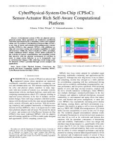
Fig. 9. The switching set of points output by our algorithm is shown projected onto fixed v and θ dimensions. Here, a single segment between two waypoints (crosses) is analyzed. The light gray states indicate the unsafe regions, whereas the dark gray states are states where the safety controller must be immediately used in order to maintain safety. The top figure is for v = 1000mm/s and bottom figure is for v = −1500mm/s. In both figures, θ is fixed at 0.
The ESCAPE toolkit uses Simulink/Stateflow as a front end.
visualized. We can, however, analyze the output set by fixing two of the dimensions (for example, v and θ) and plotting the other two dimensions. Figure 9 shows two plots of the switching set for two values of v and a fixed θ. By changing the values of v and θ, we can verify our intuition about the switching set: that going away from the waypoint-connecting line segment at high velocity will more quickly switch to the safety controller. V. R ELATED W ORK There are several algorithms and tools for computing reachable states and approximate reachable states for hybrid systems and a complete survey of these techniques is beyond the scope of this paper [11], [12], [13], [14], [15]. Work related to the PESSOA [16] tool for synthesizing embedded controllers is similar in spirit to our work. PESSOA generates a finite state abstraction of a given system and uses these abstractions for synthesizing controllers that are guaranteed certain restricted class of LTL properties such as �ϕ, �ϕ, ��ϕ and ��ϕ ∧ �ϕ0 . The controller synthesis uses earlier techniques [17], [18], [19], [20]. The finite state abstractions used in PESSOA are approximate simulations [21], [22] of the original continuous system. In contrast, the finite state abstractions we use are simulations of the original system in
the classical sense. Furthermore, our algorithm (and tool) can handle plants which are described with hybrid automata with nonlinear differential equations. To the best of our knowledge, PESSOA currently does not support such models. Checkmate [23] is a tool for verifying control systems modeled as a hybrid automaton. Checkmate computes the reach set for a linear and non-linear systems by using the flow pipe approximation technique [24] to approximate the reachable sets by a sequence of convex polyhedra. Checkmate restricts the class of hybrid systems that can be verified to polyhedral-invariant hybrid systems. Our approach, however, can verify hybrid systems without this restriction. The Simplex Architecture [2] has been applied as a sandboxing technique for various systems ranging from a fleet of remote-controlled cars [25], to a pacemaker [3], to a set of advanced aircraft maneuvers [26]. Some approaches rely on heuristics and testing to create the Simplex decision module [27]. In contrast, we propose verification based on system models. For a limited class of hybrid systems, we have previously proposed an automatic method to verify the Simplex decision module [4]. The algorithm presented in this paper accepts more general models than our previous work, and provides ways to increase reachability accuracy. Additionally, we provide the ESCAPE toolkit to synthesize automatically the decision module, rather than only checking
a decision module after it has been created, as in our previous work. VI. C ONCLUSIONS In this paper, we have addressed the problem of verifying properties of cyber-physical systems with partly unknown software components. The main technique to achieve this was to sandbox unverified components by using the Simplex Architecture. In this Simplex Architecture, however, the decision module, which switches between the unverified complex controller and verified safety controller, must be verified as correct. This paper presented a hybrid-systems reachability approach for creating this Simplex switching logic. The low-level algorithm was shown to be more general than previous approaches, with three techniques provided to improve accuracy. The approach was integrated into an end-to-end toolkit where Simulink/Stateflow models of the system can be used to create source code for the Simplex decision module, and then the toolkit was successfully applied to a skid-steer vehicle system model. The cyber-physical system sandbox approach presented in this paper, however, should not be regarded as a silver bullet that mitigates all possible system faults. For example, hardware failure is not considered in our designs, so practical systems may need to also incorporate redundancy. Additionally, as with all model-based verification techniques, the result of the verification is only as accurate as the models themselves. Runtime monitoring may be necessary to ensure that the deployed system behaves in accordance with the verification model. The proposed algorithm remains inapplicable for hybrid systems with circular explicit derivative dependencies, although this will be investigated as future work. Additionally, we will explore techniques to reduce the computation time of the method, which due to the accuracy-increasing rules, can lead to improved accuracy of the reachability computation, which will construct a less pessimistic decision module. ACKNOWLEDGMENTS The material presented in this paper is based upon work supported by the National Science Foundation (NSF) under grant numbers CNS-1016791 and CNS-1035736, and by John Deere under Award No. UIUC-CS-DEERE RPS #19. Any opinions, findings, and conclusions or recommendations expressed in this publication are those of the authors and do not necessarily reflect the views of the NSF or John Deere. R EFERENCES [1] C. Reis, A. Barth, and C. Pizano, “Browser security: lessons from google chrome,” Commun. ACM, vol. 52, pp. 45–49, August 2009. [2] L. Sha, “Using simplicity to control complexity,” IEEE Softw., vol. 18, no. 4, pp. 20–28, 2001. [3] S. Bak, D. K. Chivukula, O. Adekunle, M. Sun, M. Caccamo, and L. Sha, “The system-level simplex architecture for improved real-time embedded system safety,” in RTAS ’09: Proceedings of the 2009 15th IEEE Real-Time and Embedded Technology and Applications Symposium, 2009. [4] S. Bak, A. Greer, and S. Mitra, “Hybrid cyberphysical system verification with simplex using discrete abstractions.”
[5] T. A. Henzinger, P. W. Kopke, A. Puri, and P. Varaiya, “What’s decidable about hybrid automata?” in ACM Symposium on Theory of Computing, 1995, pp. 373–382. [Online]. Available: citeseer.nj.nec.com/henzinger95whats.html [6] G. Lafferriere, G. J. Pappas, and S. Yovine, “A new class of decidable hybrid systems,” in HSCC ’99: Proceedings of the Second International Workshop on Hybrid Systems, 1999. [7] R. Alur and D. L. Dill, “A theory of timed automata,” Theoretical Computer Science, vol. 126, pp. 183–235, 1994. [8] R. Alur, C. Courcoubetis, N. Halbwachs, T. A. Henzinger, P.H. Ho, X. Nicollin, A. Olivero, J. Sifakis, and S. Yovine, “The algorithmic analysis of hybrid systems,” Theoretical Computer Science, vol. 138, no. 1, pp. 3–34, 1995. [Online]. Available: citeseer.nj.nec.com/alur95algorithmic.html [9] D. K. Kaynar, N. Lynch, R. Segala, and F. Vaandrager, The Theory of Timed I/O Automata, ser. Synthesis Lectures on Computer Science. Morgan Claypool, November 2005, also available as Technical Report MIT-LCS-TR-917. [10] S. Mitra, “A verification framework for hybrid systems,” Ph.D. dissertation, Massachusetts Institute of Technology, Cambridge, MA 02139, September 2007. [Online]. Available: Available at http://people.csail.mit.edu/mitras/research/thesis.pdf [11] E. Asarin, O. Bournez, T. Dang, and O. Maler, “Approximate reachability analysis of piecewise-linear dynamical systems,” in Hybrid Systems: Computation and Control, ser. LNCS, B. Krogh and N. Lynch, Eds., vol. 1790. Hybrid Systems: Computation and Control, 2000, pp. 20–31. [12] T. A. Henzinger, P.-H. Ho, and H. Wong-Toi, “Hytech: A model checker for hybrid systems,” in Computer Aided Verification (CAV ’97), ser. LNCS, vol. 1254, 1997, pp. 460–483. [13] J. Bengtsson, K. G. Larsen, F. Larsson, P. Pettersson, and W. Yi, “UPPAAL in 1995,” in Tools and Algorithms for Construction and Analysis of Systems (TACAS), 1996, pp. 431–434. [14] A. Chutinan and B. Krogh, “Computational techniques for hybrid system verification,” in Auto-matic Control, IEEE Transactions, pp. 64–75. [15] G. E. Fainekos and G. J. Pappas, “Robustness of temporal logic specifications for continuous-time signals,” Theoretical Computer Science, vol. 410, no. 42, pp. 4262–4291, 2009. [16] M. M. Jr., A. Davitian, and P. Tabuada, “Pessoa: A tool for embedded controller synthesis,” in Proceedings of the 22nd International Conference on Computer Aided Verification, 2010. [17] R. Kumar and V. Garg, “Modeling and control of logical discrete event systems.” Kluwer Academic Publishers, 1995. [18] C. Cassandras and S. Lafortune, “Introduction to discrete event systems.” Kluwer Academic Publishers, 1999. [19] L. de Alfaro, T. A. Henzinger, and R. Majumdar, “Symbolic algorithms for infinite-state games,” in CONCUR 01: Concurrency Theory, 12th International Conference, 2001. [20] R. Alur, T. Henzinger, O. Kupferman, and M. Vardi, “Alternating refinement relations,” in Proceedings of the 8th International Conference on Concurrence Theory. Springer, 1998. [21] Paulo Tabuada, Verification and Control of Hybrid Systems: A Symbolic Approach. Springer, 2009. [22] A. Girard and G. J. Pappas, “Approximation metrics for discrete and continuous systems,” in IEEE Transactions on Automatic Control, 2005. [23] J. Kapinski and B. H. Krogh, “A new tool for verifying computer controlled systems,” in IEEE Conference on Computer-Aided Control System Design, pp. 98–103. [24] A. Chutinan and B. H. Krogh, “Verification of polyhedral-invariant hybrid automata using polygonal flow pipe approximations,” LNCS, vol. 1569, pp. 76–91, 1999. [Online]. Available: citeseer.nj.nec.com/chutinan99verification.html [25] T. L. Crenshaw, E. Gunter, C. L. Robinson, L. Sha, and P. R. Kumar, “The simplex reference model: Limiting fault-propagation due to unreliable components in cyber-physical system architectures,” in RTSS ’07, Washington, DC, USA, 2007, pp. 400–412. [26] D. Seto, E. Ferreira, and T. F. Marz, “Case study: Development of a baseline controller for automatic landing of an f-16 aircraft using linear matrix inequalities (lmis),” Technical Report Cmu/ sei-99-Tr-020. [Online]. Available: citeseer.ist.psu.edu/ 606539.html [27] E. D. Ferreira and B. H. Krogh, “Switching controllers based on neural network estimates of stability regions and controller performance,” in Lecture Notes on Computer Science, Special Issue: Hybrid Systems VI. Springer Verlag, 1999.