Scalable architecture and query optimization ... - Cs.UCLA.Edu

Scalable Architecture and Query Optimization for Transaction-time DBs with Evolving Schemas Hyun Jin Moon* NEC Labs America [email protected]

Carlo A. Curino* MIT [email protected]

Carlo Zaniolo UCLA [email protected]

ABSTRACT

General Terms

The problem of archiving and querying the history of a database is made more complex by the fact that, along with the database content, the database schema also evolves with time. Indeed, archival quality can only be guaranteed by storing past database contents using the schema versions under which they were originally created. This causes major usability and scalability problems in preservation, retrieval and querying of databases with intense evolution histories, i.e., hundreds of schema versions. This scenario is common in web information systems and scientific databases that frequently accumulate that many versions in just a few years. Our system, Archival Information Management System (AIMS), solves this usability issue by letting users write queries against a chosen schema version and then performing for the users the rewriting and execution of queries on all appropriate schema versions. AIMS achieves scalability by using (i) an advanced storage strategy based on relational technology and attribute-level-timestamping of the history of the database content, (ii) suitable temporal indexing and clustering techniques, and (iii) novel temporal query optimizations. In particular, with AIMS we introduce a novel technique called CoalNesT that achieves unprecedented performance when temporal coalescing tuples fragmented by schema changes. Extensive experiments show that the performance and scalability thus achieved greatly exceeds those obtained by previous approaches. The AIMS technology is easily deployed by plugging into existing DBMS replication technologies, leading to very low overhead; moreover, by decoupling logical and physical layers provides multiple query interfaces, from the basic archive&query features considered in the upcoming SQL standards, to the much richer temporal XML/XQuery capabilities proposed by researchers.

Algorithms, Design, Experimentation, Management, Performance

1.

INTRODUCTION

Archiving past database information and supporting temporal queries over historical databases have long been recognized as critical requirements for advanced Information Systems [31], and the urgency of this requirement is further exacerbated by the accountability obligations of web information systems that reach a wide public [16]. These considerations that, in the past, have motivated temporal database research, are now starting to penetrate in the commercial world, as testified by commercial support for notions such as ‘flashback’ [1] and the new temporal constructs pushed in the SQL standards by the main DBMS vendors [2]. Many technical challenges arise in this context: thus, in addition to the problems that have been explored and largely solved by previous research on transaction-time databases, we now find the problem that over time, databases evolve not only in their contents, but also in their schemas. Schema evolution, which represents a serious problem for traditional information systems [38, 25], has become even more critical for web information systems, where the need to preserve and account for previously published information is also very acute. In fact, recent studies show that web information systems undergo frequent schema changes: Wikipedia has experienced more than 170 schema changes in its 4.5 years of lifetime [16]. The scientific repositories of ’big science’ projects experience similar issues: for instance, the Ensembl Genetic DB over 400 schema versions in nine years of life [15]. In order to achieve faithful preservation, archival database systems must preserve their data using the schema version under which they were originally stored since migration is in general not information preserving, and this causes major usability issues. Indeed, Categories and Subject Descriptors to issue queries on historical data the users would need to understand and query many schema versions, potentially hundreds in the H.2.1 [Database Management]: Logical Design—Schema; H.2.8 [Database Management]: Database applications—Temporal databases real scenarios as above. The PRIMA system [28] was the first to address this difficult issue by enabling the user to pose a query Q against a chosen schema ∗ Work done while authors are at UCLA (typically the current one) and then having the system to automatically: (i) determine the applicable schemas according to the temporal condition in Q, (ii) translate Q into an equivalent query against each applicable schema, and (iii) combine these queries to produce results conforming to the schema queried by the user. The Permission to make digital or hard copies of all or part of this work for data model and query language exploited in PRIMA were based on personal or classroom use is granted without fee provided that copies are not made or distributed for profit or commercial advantage and that copies XML and XQuery that has been proved very effective for expressbear this notice and the full citation on the first page. To copy otherwise, to ing complex temporal queries [43]. However the implementation of republish, to post on servers or to redistribute to lists, requires prior specific this solution on XML native database systems lacks scalability and permission and/or a fee. leads to poor performance, particularly when many schema verSIGMOD’10, June 6–11, 2010, Indianapolis, Indiana, USA. sions are involved. Two particularly serious sources of inefficiency Copyright 2010 ACM 978-1-4503-0032-2/10/06 ...$10.00.

207

ness requirements and operating environment, the schema receives the following sequence of modifications. As the company seeks to uniformly manage the department information, the DBA applies the first modification at time T2 , which merges two tables engineerpersonnel and otherpersonnel, producing schema V2 . With the growth of the company, the need for storing more information about departments leads to a new schema version V3 , which occurred at time T3 . In V3 , a new table dept was created, which stores department number, department name, and the manager, for each department. After a while, due to a new government regulation, the company is now required to store more personal information about employees. At the same time, it is required to separate employees’ personal profiles from their business-related information to ensure privacy. For these reasons, the database layout is changed at T4 , to the one in version V4 , where the information about the employee is enriched and divided into two tables: empbio, storing the personal information about the employee, and empacct, maintaining business-related information about the employee. Finally, the company chooses to change the compensation policy. To better motivate employees, the salary becomes dependent on the individual performance, rather than on his or her job title. This is supported by moving the salary attribute to the empacct table, and dropping table job. Also, employee name was split into first name and last name to make it easier to sort employees by their last name. These changes, which are applied at T5 introduced the last schema version, V5 .

Table 1: Running Example: Schema evolution in employee DB V1

V2 V3

V4

V5

Schema Versions engineerpersonnel (empno, name, hiredate, title, deptname) otherpersonnel (empno, name, hiredate, title, deptname) job (title, salary) empacct (empno, name, hiredate, title, deptname) job (title, salary) empacct (empno, name, hiredate, title, deptno) job (title, salary) dept (deptno, deptname, managerno) empacct (empno, hiredate, title, deptno) job (title, salary) dept (deptno, deptname, managerno) empbio (empno, sex, birthdate, name) empacct (empno, hiredate, title, deptno, salary) dept (deptno, deptname, managerno) empbio (empno, sex, birthdate, firstname, lastname)

Ts

Te

T1

T2

T2

T3

T3

T4

T4

T5

T5

now

are: (i) the complexity of rewriting temporal XQuery statements, and (ii) the lack of reliable techniques for optimizing these queries. The new archival system called AIMS1 that we propose in this paper overcomes these problems with two-tier architecture whereby the lower level achieves dramatic improvements in scalability and performance by using a relational storage engine and specialized temporal optimization techniques are exploited. In particular, for the frequently required task of coalescing historical data [8] fragmented by schema evolution, our system introduces a novel technique that delivers major performance improvement over the best algorithm up to date [47]. Furthermore, this two-tier architecture allows us to provide multiple query interfaces, ranging from the system-versioned tables [2] proposed in the new SQL/Temporal standard, to the XML/XQuery query interface presented in previous systems, whereby the support for schema evolution and the optimization of queries is managed uniformly in the physical layer. Finally, to enable the usage of our system in practice we implemented it as an extension of the MySQL master/slave replication technology—a history-enabled slave. This provides us with the capabilities of storing the history of the DB content, simply observing the MySQL binary log—leading to minimal performance overhead in the production database. Organization The paper is organized as follows. After presenting our running example in the following subsection, we discuss previous works in Section 2. In Section 3, we discuss the background of our work, which includes considered schema changes, temporal data model and query language based on both relational and XML. We then present the architecture of AIMS, which is relational-based physical layer of transaction-time DB with evolving schemas in Section 4. Section 5 is devoted to the discussion of fragmented histories in schema evolution and our temporal coalescing method, CoalNesT. We present experimental validation of the proposed techniques in Section 6, and conclude the paper in Section 7.

1.1

2.

Running Example

We illustrate the schema evolution of an employee database, which is used as a running example in the rest of the paper. Table 1 outlines the five-versions evolution history of our example. At the establishment of the database at T1 , schema version V1 initially has three tables: engineerpersonnel, otherpersonnel and job. The first two store information about the engineers and the rest of the personnel, respectively. The job table relates the employee job titles to the corresponding salaries. Now, due to the changes in busi1

PREVIOUS WORK

There has been extensive work on schema evolution in the context of OODB [6, 32, 11, 12, 13]. More recently, schema evolution has also been studied in the framework of model management [7, 27], and through schema mapping and query rewriting [17, 18]. None of these works, however, considered the management of historical data. Within the temporal databases, there has been several proposal for schema evolution support [26, 5, 9, 39]. Their approaches can be summarized as: (i) preserving schema versions by means of timestamps, (ii) extending SQL to express the query target schema version, and (iii) supporting queries by migrating data to the queried schema version. See [35, 33] for in-depth surveys. PRIMA system [28] goes beyond these by automating the process of adapting complex temporal queries issued on a single schema version over multiple schema versions, but it suffers from limited performance, no support for temporal coalescing and limited query interface. These problems are discussed and addressed in this paper. Efficient implementations of coalescing have also been studied in depth in temporal databases literature. Several approaches have been proposed to support coalescing in SQL, which are based on: (i) multiple nested “NOT EXISTS” clauses and self-joins [45], (ii) COUNT aggregates [40], and (iii) recursive SQL queries [21]. Unfortunately, these approaches suffer from performance limitations. Recently, Zhou et al. [47] have proposed two coalescing methods based on a single scan of their input table, improving the performance substantially over existing approaches. One is single scan coalesce (SSC) that is based on SQL:2003 OLAP features and the other is a coalescing technique based on user-defined aggregates. The algorithm common in the two methods is as follows: given a sequence of transaction-time tuples sorted by the start time, it makes one pass, incrementing a counter each time it sees the start time, and decrementing it for each end time observed. Whenever

Archival Information Management System

208

Table 2: Schema Modification Operators (SMOs) SMO Syntax

Table 3: H-Tables Example: empacct_salary table empno salary ts te 10002 40000 1988-02-20 1989-02-20 10002 42010 1989-02-20 1990-02-04 10002 42525 1990-02-04 1991-02-04 ... ... ... ... 10003 43162 1988-07-13 1989-07-13 ... ... ... ...

¯ CREATE TABLE R (A) DROP TABLE R RENAME TABLE R INTO T COPY TABLE R INTO T MERGE TABLE R , S INTO T PARTITION TABLE R INTO S WITH cond, T ¯ B ¯ ), T (A, ¯ C ¯) DECOMPOSE TABLE R INTO S ( A, JOIN TABLE R , S INTO T WHERE cond ¯ )] INTO R ADD COLUMN C [ AS const|f unc(A DROP COLUMN C FROM R RENAME COLUMN B IN R TO C

Attribute Level Timestamping In the transaction-time DB literature two main approaches have been proposed: Tuple Level Timestamping (TLT), and Attribute Level Timestamping (ALT). They differ based on the granularity of the timestamping, while they provide equivalent expressivity. ALT is also known as temporally grouped model and proved to be superior [14], since it leads to less redundancy in the storage and minimal need for temporal coalescing during query answering.

the counter becomes zero, it produces a coalesced tuple for one or more overlapping tuples. In [47], it is shown that both runs in linear time, which is the best result available to date. The temporal coalescing algorithm CoalNest proposed in this paper provides an even more efficient way of dealing with coalescing for data fragmented by schema changes. We also mention Dyreson [19], who has proposed an efficient coalescing strategy, particularly relevant in the context of validtime databases. Vassilakis [42] proposed an optimization technique for coalescing, reducing the coalescing workload using prefiltering predicates added to the query. Lastly, Al-Kateb et al. [4] have proposed an efficient coalescing technique based on an augmented temporal data model. This technique is similar to the one we presented here in that it exploits additional information for efficient coalescing. However, these two approaches significantly differ in the technical aspects and goals. They aim at improving project-columns-and-then-coalesce within a single table in TLT data model, whereas we address coalescing of tuples fragmented due to schema changes, spanning over multiple tables for ALT data model. To the best of our knowledge, our approach is the first addressing the problem of history fragmentation and coalescing due to schema evolution. Other relevant works on fragmented history management appeared in [36, 29]. Challenges in the design of efficient transaction-time DBMS have been addressed in [22, 23, 24]. These approaches provide enabling technologies for transaction-time DB, but do not take into account schema evolution. Recently, column-store DBMS [41] have been used for storing semantic web data in a vertically partitioned format [3]. This approach is somewhat similar to H-Tables, except for the explicit management of the temporal dimension. An interesting research direction is to employ column-store as a physical layer of temporal databases, which is not explored in this paper.

3.

Physical storage: H-Tables The AIMS physical storage layer constructs on a ALT-inspired data organization firstly introduced in [43]. In the following, we explain H-Tables using a relation empacct of the schema V5 reported in Table 1: empacct (empno, hiredate, title, deptno, salary) The history of the empacct relation is stored into H-Tables as: (i) a key table, (ii) the attribute history tables, and (iii) a global table as follows. (i) The key table: empacct_empno (empno, ts, te) Since empno will not change over time2 , the interval(ts, te) in the key table represent the interval in which the tuple was stored in the corresponding snapshot DB. (ii) Attribute history tables: empacct_hiredate (empno, hiredate, ts, te) empacct_title (empno, title, ts, te) empacct_deptno (empno, deptno, ts, te) empacct_salary (empno, salary, ts, te) Appropriate indexing of H-tables can produce very efficient joins of these relations, as shown in [43]. A sample content of the empacct_salary table is shown in Table 3. (iii) Global table: relations (relationname, ts, te) recording all the relation history in the database schema, i.e., the time spans covered by the various tables in the database.

3.2

PRELIMINARIES

In this section, we briefly introduce notions about schema evolution and temporal data models required for the rest of the paper.

3.1

Temporal Query Languages

As previously introduced, AIMS provides support for multiple query languages, and allow ease of extensibility. In the remainder of this section we summarize the two main query language currently supported: SQL/Temporal standard, and XML/XQuery.

SQL/Temporal Standard

Schema Evolution and Physical Storage

Schema Modification Operators There are several ways to model schema changes in relational databases [37, 26, 17], and we use schema modification operators (SMOs) [17] to model schema changes, which is summarized in Table 2. The SQL-inspired syntax is self-explanatory to the purpose of this paper, while the interested reader can refer to [17] for a detailed and formal presentation of the SMOs and their capabilities. In our system, users describe schema evolution using SMOs, which becomes the input of our query rewriting component.

209

The major DBMS vendors are collaborating to include in the upcoming ISO SQL standard new temporal features [2], as requested by their respective customer bases. The SQL/Temporal draft includes both valid-time and transaction-time features, which are renamed for marketability as business-time and system-time, respectively. The current version of the standard provides only basic temporal features, limited in fact to simple temporal queries: range and snapshot queries. These limitations are dictated by the technological challenges to support a richer query language. Further2

ArchIS design builds on the assumption that keys (e.g., empno) remain invariant in the history. Otherwise, system-generated surrogate keys are used.

more, DBMS vendors have no plans to support schema evolution in their initial product releases. The AIMS system focuses on the transaction-time features and supports them also under schema evolution. We provide an example of such language in the following query: Query Q1: (SQL/Temporal) Find empno of employees who made more than 120K as of 2004-07-01. SELECT empno FROM empacct WHERE salary > 120000 AS OF SYSTEM TIME 2004-07-01; In Section 4, we will describe how the system support this query language, by compiling and optimizing it into equivalent queries operating on our H-Table based physical layer.

Figure 1: AIMS Two-Tier Architecture This illustrate the need for a richer query language, in those scenarios in which the basic features being standardized in SQL are not enough for the user’s needs. V-Document have been naturally extended to support schema evolution in [28]. Modifications in the schema of the snapshot database, are viewed as new branches of the XML tree structure. The timestamp values guarantee an unambiguous association among tuples, tables and schema versions. Therefore, this general representation, named MV-Document (Multi-schema-version V-Document), is capable of providing a coherent logical view of the history of database subject to schema evolution.

Temporal XQuery The above introduced SQL/Temporal query language provides only basic temporal features, but it lacks the expressivity often needed to fully exploit the historical content of a transaction-time DB. In order to provide a more advanced query interface we follow the approach of [43, 28], thus exploiting the expressive power of XQuery as query language. It has been shown that XML and XQuery can naturally model and query histories of relational databases in a temporally grouped representation [34, 30, 43]. We introduce an XML-based temporal model, called V-document [43], and its extension MV-document [28] that allows modeling and querying of temporal databases with evolving schemas. This operates as a logical view of data physically stored in the H-Table based storage solution described above. The Attribute Level Timestamped history of a database can be stored in an XML document organized as follows: /db/table-name/row/column-name Each XML element, representing respectively: database, tables, tuples, and columns, has two XML attributes, start-time (ts) and end-time (te), representing respectively the (transaction-) time in which the element was added to the database and the time in which was removed. A special value “now" is used to represent the end time for those tuples that are still active in the database. XQuery is used, without any extension, as a powerful temporal language over this representation. This is possible due to the expressive power of XQuery, which is Turing-complete [20]. Let us first show the XQuery equivalent of query Q1 above:

4.

SYSTEM ARCHITECTURE

AIMS architecture is shown in Figure 1. The architectural choice of decoupling the logical and physical layers leads to major performance improvements over existing approaches, as shown in the experimental Section 6. Furthermore, this two-tier architecture allows us to factorized in the physical layer the management of schema evolution and sophisticated temporal query optimizations, while the logical layer offers extensibility at the query interface level, as demonstrated in Figure 1. The AIMS system (i) receives input SQL/Temporal or XQuery queries, (ii) translate/compile such queries into SQL (or SQL/XML) on the underlying H-tables, (iii) rewrite the SQL on H-Table across multiple schema versions, and (iv) optimize the query to achieve better execution performance.

4.1

Input Query Compilation

Step (ii) depends on the input query language; syntactical translations are possible among various temporal query languages. The current prototype of the AIMS system implements two interfaces described in the following paragraphs: SQL/Temporal and XQuery. Thanks to the limited set of temporal features of SQL/Temporal, it is easy to syntactically detach the SQL body of the query and its temporal specification (i.e., the AS OF SYSTEM TIME construct shown in query Q1). The rewriting of the SQL body, expressed on the snapshot schema, to the corresponding H-Table schema is easily implemented by means of schema mapping and query rewriting [17]. The temporal specification is managed separately, and is used to generate corresponding conditions on various H-Tables. The query Q1 of Section 3.2 is, thus, automatically translated in the following query Q1h on H-Tables.

Query Q1x: XQuery equivalent to query Q1 for $x1 in doc("emp.xml")/db/empacct/row [salary>120000 and @ts ‘2004-07-01’] return $x1/empno/text() The following query Q11 represent a more complex temporal query3 , which cannot be captured by SQL/Temporal extension of SQL, but is naturally represented in XQuery: Query Q11x: (XQuery) Find empno of employees who worked with employee 1 (in the same department), for an overlapping period of time of at least two years.

Query Q1h: H-Tables rewriting of Q1.

for $x1 in $db/empacct/row[empno=’1’]/deptno, $x2 in $db/empacct/row/deptno where $x1=$x2 and $x1/../empno!=$x2/../empno and overlapdays($x1, $x2) > 730 return $x2/../empno/text()

SELECT R0.empno FROM empacct_salary R0 WHERE R0.salary>120000 AND R0.ts’2004-07-01’;

3 Queries are numbered according to how they are grouped and used in the experimental section.

To support XML/XQuery view of the data introduce above, we exploit the fact that the XML V-Document model has a direct map-

210

ping to the underlying relational H-Tables (which can be viewed as the shredding of the XML document). In order to compile XQuery queries into equivalent SQL/XML on H-Tables we implemented in the prototype and extended version of the algorithm of [43]. Notice that this is not a general purpose translation of XML/XQuery to SQL, but a translation of the subset of XQuery used to express relational temporal queries4 , on a specific relational representation. This allows for simplifications and optimizations of the general problem that make the translation simple and fast. As a result, the system is capable of translating the query Q1x into the above query Q1h5 .

4.2

complex temporal queries spanning multiple schema versions are difficult to optimize with general-purpose optimizers, due to their agnostic approach to time. In this subsection, we focus on an important class of temporal queries not properly optimized by the optimizer of a DB2. For those queries, a temporally-aware optimized can achieve significantly better performance, by exploiting the temporal characteristics of the query, as shown in the following. In our transactiontime DBs, historical data is stored under the schema version following the original-schema-archival policy. Therefore, the interval of temporal data, i.e., [ts, te), is contained within the interval of the schema version. We make this property explicit by using “check constraints” (in case of DB2) which are usually successfully exploited by the optimizer in improving the query execution plans. However, if the value comparisons of queries involve the results of functions or case statements, then the DB2 optimizer fails to optimize the query, which occurs often in temporal queries where time intersection of tuples is evaluated by means of min/max scalar functions or case statement (e.g., CASE WHEN a>b THEN a ELSE b END). To overcome this limitation, we implement the temporalspecific optimizations in our system, which generates the temporal queries that are already optimized and pass them to the underlying RDBMS. Please consider the following example queries.

Query Rewriting in the Physical Layer

In the following we describe the rewriting between schema versions. Input queries, expressed on a selected schema version (often the current one), are translated into the equivalent SQL queries over H-Tables, by the algorithms mentioned above. The resulting SQL queries might refer to portions of the history stored under previous schema versions. The temporal specification of each query is analyzed and the query is rewritten from the target schema version (the one queried) to the source schema versions (i.e., those valid during the timespan specified in the query). The H-tables-based representation is completely transparent to the user, who model evolution in terms of Schema Modification Operators on the corresponding snapshot schema. Thus, the actual rewriting is performed as follows: (i) H-Table queries on the target schema version are transformed into queries over snapshot tables, (ii) rewriting is performed according to the SMO specification on the snapshot DB, and (iii) the produced rewriting is transformed back into the H-Table format. Thanks to the simple mapping between H-Tables and the corresponding snapshot tables (i) and (iii) are very simple (and thus fast) rewriting step. Furthermore, (ii) is a pure rewriting between snapshot schemas, which is highly optimized and thus efficient, as shown in [17]. The overall rewriting time is kept low enough not to significantly impact the overall execution time. Furthermore, in the experimental Section 6 we validate this approach showing scalability on long evolution histories and a significant performance improvement when comparing AIMS with the results obtained by previous systems [28]. Below, we show the result of rewriting query Q1h, expressed on the H-Tables of schema version V2 , into schema version V1 , the schema valid at the time of interest for the query: ’2004-07-01’.

Query Q15: Find titles of all employees at 2001-07-016 for $x1 in $db/empacct/row, $x2 in $x1/title[@ts "2001-07-01"] return {$x1/empno/text(), $x2/text()} When we rewrite this query, engineerpersonnel_title and otherpersonnel_title are needed for answering the query, but empacct_title is not necessary, as its tuples have ts > 2002-01-01 that can never satisfy the condition ts 120000 AND R0.title=R1.title AND R0.ts’2004-07-01’ AND R1.ts’2004-07-01’; The following subsection discusses further temporal-specific optimizations required to achieve the performance requirements of real-world data archives.

4.3

Temporal Query Optimization

RDBMS optimizers are usually good at exploiting given integrity constraints to achieve semantic query optimization. These techniques prove to be highly effective in many common scenarios, but

Here, engineerpersonnel_title, otherpersonnel_title, job_salary are needed, but empacct_title and empacct_salary can be excluded, for the same reason above. We omit rewritten queries due to the limited space.

5.

TEMPORAL COALESCING

Temporal coalescing is a common and expensive data restructuring operation applicable to temporal databases, similar to duplicate elimination in non-temporal databases. Coalescing merges timestamps of adjacent or overlapping tuples that have identical attribute values [8]. In this section, we discuss the requirement of temporal coalescing in transaction-time database with evolving schemas, and present a novel coalescing method called CoalNesT.

5.1

Coalescing for Schema Evolution

H-tables, being based on a temporally grouped data model [14], significantly reduces the need for coalescing, as data are already stored in a coalesced format, for each individual attribute [43] (see Section 6.2, H-Tables vs. TLT). With schema evolution, however,

4

It is easy to enforce the constraint on the valid statement in the parsing phase. 5 We omit SQL/XML publishing functions in the SELECT clause of the translated SQL queries (e.g., XMLELEMENT, XMLATTRIBUTE, XMLAGG), for the sake of a concise presentation. Full translation can be found in [43].

6 Queries are numbered based on the way they are used in the experiment. See Table 7.

211

engineeringpersonnel_title: V1 , [2001-01-01, 2002-01-01) empno title ts te tfs lastflag 10001 asst. 2001-04-01 2001-10-01 2001-04-01 true 10001 staff 2001-10-01 2002-01-01 2001-10-01 false empno 10002 10003 empno 10001 10003 10003

schema time

title staff asst. staff

CSVTDB2

T3

otherpersonnel_title: V1 , [2001-01-01, 2002-01-01) title ts te tfs lastflag asst. 2001-04-01 2001-10-01 2001-04-01 true asst. 2001-04-01 2002-01-01 2001-04-01 false empacct_title: V2 , [2002-01-01, now] ts te tfs 2002-01-01 now 2001-10-01 2002-01-01 2002-04-01 2001-04-01 2002-04-01 now 2002-04-01

TDB 1 '

V2

TDB 2

T2

TDB 1

V1

lastflag true true true

T1 T1

TDB1

T2

TDB2

T3

data time

Figure 2: NTH-Tables example

Figure 3: Transaction-time DB under V1 and V2

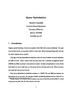
we face a new need for coalescing: when the schema evolves, data are stored under the original schema version (to guarantee perfect archival quality). As a consequence, the history of a data value might be partitioned under two schema versions, which will often need to be coalesced back during query answering. Consider the example7 in Figure 2. For the period of [2001-1001, now), the employee 10001 has the title of staff. On 2002-0101, however, schema version V1 is evolved into V2 , and thus this record is broken down into two fragments: [2001-10-01, 2002-0101) stored in engineeringpersonnel_title and [2002-01-01, now) in empacct_title. Since migrating data into the new schema version might lead to data losses we store the history under the original schema version. This policy enables perfect archival quality, but it brings up a new issue in query answering: the need for coalescing tuples fragmented by schema changes. Consider the example in Figure 2 that shows the tuples that are fragmented, due to the schema change— MERGE TABLE between V1 and V2 in Table 1. The records of employee 10001 and 10003 are fragmented at time 2002-01-01, i.e., when schema changed from V1 to V2 . A query asking the title history of employee 10001 on a period overlapping the schema change point requires coalescing the two fragments. This is highly desirable to avoid unexpected duplicates and a not-intuitive query answering semantics. Furthermore, without coalescing, we would not be able to correctly answer queries predicating about the length of period such as, “Find employees who worked as an assistant staff for one year or more”, since the fragmentation induced by schema evolution would make us miss employee 10003 in the answer.

friendly query interface, which is much more convenient than manually writing complex temporal queries spanning on each of T DBi under Vi (1 ≤ i ≤ k). In order to further shield the users from the underlying schema evolution, we incorporate temporal coalescing into the physical layer and also the above semantics rather than having users to handle it. We coalesce the original SV T DBk into CSV T DBk , as in Figure 3. Thus, the user queries posed over schema version Vk will be executed against CSV T DBk which is the (conceptually) migrated, unioned, and coalesced history of the data.

5.2

5.3

Coalesce by Nested Timestamps (CoalNesT)

Even with the most efficient temporal coalescing technique available to date, i.e. SSC [47], it would take linear time in the size of the data to perform coalescing. Thus we develop a highly efficient coalescing algorithm, CoalNesT, which, based on nested timestamps, achieves a significant performance improvement.

5.3.1

Query Answering Semantics

Users are allowed to query database histories under multiple schema versions by posing queries on a target schema version, as if the whole history was stored under that schema version. This is formalized by the query answering semantics of [28] using the approach described in [44]: given a target version Vk , we migrate each database T DBi under Vi (i ≤ k) to Vk according to the schema mappings and obtain T DBi0 valid on Vk . The input query is evalu0 ated on the union of T DB10 , T DB20 , ..., T DB(k−1) , T DBk . This union, called single version transaction-time database (SVTDB), represents the entire history of the transaction-time database migrated under Vk . We name SV T DB under Vk as SV T DBk . Figure 3 shows a case of k=2. Note that no migration is performed to answer the query. This formalization capture our query answering semantics, while the implementation is based on query rewriting. By supporting this semantics by means of rewriting we allow users to write queries on Vk as if they were executed on SV T DBk . This provides a user7 The two rightmost columns, tfs and lastflag, will be introduced later in Section 5.3 and can be ignored now.

212

Nested Timestamps

In addition to the four attributes in regular H-Tables, we add two extra attributes, which are called nested timestamps: tfs and lastflag. The timestamp tfs captures the original start time of a record lifetime, regardless of fragmentation introduced in the middle. To be specific, tfs (i.e. time-first-start) of a tuple r indicates ts of r’s coalesced tuple rc , which is created by coalescing r with other tuples. Similarly, lastflag tells whether the record is the last fragment of the tuple: lastflag of a tuple r tells whether r is the tuple that ends rc (true), or not (false). With nested timestamps, H-Tables are extended to Nested Timestamp H-Tables (NTH-Tables) as follows. Relation (key, value, ts, te, tfs, lastflag) Our measurements show that the nested timestamps use 22 to 25% of additional storage for the data set in Table 6. Figure 2 shows how nested timestamps are maintained before and after a schema change in NTH-Tables. In principle, when a tuple is fragmented by a schema change, original-schema-archival policy requires the first half to be archived under the old schema version and the second half under the new schema version. For the first half, we keep tfs value as is, and set lastflag false, to indicate that there’s another tuple that follows this. For the second one, we set lastflag true to indicate that this is the last tuple, and set its tfs by copying the tfs value of the first half.

5.3.2

CoalNesT

Based on these nested timestamps, we devise an efficient coalescing algorithm, called Coalesce by Nested Timestamps (CoalNesT). The main idea of CoalNesT is that a last tuple (i.e. whose lastflag=true) tells us the timespan of its coalesced tuple, by its [tfs, te).

R1 r1

r2 r3

R2 r4

S1 s1

s2 s3

R3

r5

16 joins R2

R3

R4

R1

R2

R3

R4

S1

S2

S3

S4

S1

S2

S3

S4

r6

S2 s4

S1

R3

S2

S3

Original CoalNesT

Table 4: Joins performed by unoptimized CoalNesT s1 s2 s3 s4 s5 r1 R1./S1 No R1./S2 r4 R2./S2 R2./S2 r2 No No No r5 No No r3 R2./S1 No R2./S2 r6 R3./S2 R3./S2

5 joins R2

R1

S1

S2

R3

S3

Optimized CoalNesT

Figure 5: Number of joins performed by CoalNesT

r1 r2 r3

In other words, last tuple works as a coalesced tuple and coalescing can be done simply by looking up the tuples with lastflag=true. The CoalNesT works quite intuitively and performs the following steps: i) search for last tuples in the source schema versions, ii) migrate tuples into the target schema version, iii) compute their union, and iv) execute the input query on it. When JOIN TABLE is among the SMOs used, CoalNesT must perform temporal joins8 [46] to execute the query answering semantics: we migrate historical data into the queried schema version, by executing SMOs on the historical data. In CoalNesT, only last tuples are used, and then it checks for temporal overlap using [tfs,te) and tests value equality. By joining tables R and S, the join output tuples get the following attributes: ts as max(R.ts, S.ts), te as min(R.te,S.te), tfs as max(R.tfs,S.tfs), and lastflag as true. Consider the example in Figure 4. It shows version history of two tables R3 and S2: R1 evolved into R2 (say, by RENAME TA BLE ), and again into R3 (say, by PARTITION TABLE into R3 and R4, which is not shown for brevity). Similarly, S1 evolved into S2 (say, by COPY TABLE). R2 and S2 were introduced at the same time. Below the tables, sample tuples (e.g., r1, r2, s1) are shown as lines, drawn with [tfs, te) timespan. Note that we chose to draw with this timespan rather than [ts,te) for sake of explanation. The lines that end with an arrow (i.e., r1, r3, r4, r6, s1, s3, s4, s5) are the last tuples whose lastflag=true, and the lines that end with a circle (i.e., r2, r5, s2) are non-last tuples. Note that r3, r6, and s3 are continuations of r2, r5, and s2, respectively. Each tuple is stored in exactly one table: r1 and r2 in R1, r3, r4, and r5 in R2, r6 in R3, s1 and s2 in S1, s3, s4, and s5 in S2. Now assume that we create a new schema version with a single table X1 as a JOIN TABLE of R3 and S2, and assume that a query is posed on X1. In order to answer it, we join the history of R1, R2, and R3 with S1 and S2, to create history under X1. We next show how this is done in CoalNesT. Since CoalNesT with other SMOs require simple selection of last tuples and their migration, we focus on JOIN TABLE. After selecting and migrating R1 and R2 into R3, and S1 into S2, we have the history to be joined, which remain essentially the same as in Figure 4. The tuple-pair joins are shown in Table 4. Non-last tuples (i.e., s2, r2, r5) are rejected before joins, and for the remaining last tuples, we perform temporal joins pairwise. We therefore perform six joins, namely R1./S1, R1./S2, R2./S1, R2./S2, R3./S19 , and R3./S2.

9

9 joins R2

R1

s5

Figure 4: CoalNesT Example

8

4 joins

R1

Table 5: Joins performed by optimized CoalNesT s1 s2 s3 s4 s5 R1./S1 R1./S1 No r4 R2./S2 R2./S2 r5 R2./S2 R2./S2 R1./S1 R1./S1 No No No R2./S2 No R3./S2 r6

5.3.3

Optimized CoalNesT

The main problem of above CoalNesT algorithm is, given JOIN 2 TABLE , we need to join O(n ) table-pairs. For instance, to join R and S, each of which has R1, R2, ..., Rn, and S1, S2, ..., Sm, as the historical source tables, we need to perform (R1 ∪ R2∪ ...∪ Rn) ./ (S1 ∪ S2 ∪ ...∪ Sm), which expands to nm partial joins, or asymptotically speaking, O(n2 ) joins. This is shown in the left hand side of Figure 5. This is unavoidable, since each table-pair can potentially overlap on their [tfs, te), and contribute to the query answer, because tfs is poorly bounded and can be any time instance between beginning of history and te. In order to reduce the number of joins needed, we observe the following fact: the unoptimized algorithm utilizes only the last tuples, while non-last tuples (i.e., whose lastflag=false) are ignored without being utilized. We can exploit these non-last tuples, to develop an optimized version of CoalNesT, which reduces the number of joined table-pairs down to O(n). The idea is that if history of two tuples join, they join between two tables that have overlapping schema version timespan. For instance, in Figure 4, the join of R1 with S2 is not really necessary. We can replace r1./s3 with r1./s2 that produces the same join result because a non-last tuple s2 is temporally contained in the last tuple s3 in S2. In this way, we can avoid cross-version joins (i.e., R1./S2, R2./s1, R3./S1) and perform only intra-version joins (i.e., R1./S1, R2./S2, R3./S2). To implement this, we check the temporal overlap based on [ts,te), rather than [tfs,te). In this way, r1 and s2 would temporally overlap on [ts,te), but r1 and s3 would not. By avoiding cross-version joins, our join graph reduces to a monotonic join graph [10], where the number of joins remain linear in the number of joined tables, decreasing the cost of JOIN TABLE from O(n2 ) to O(n). Figure 5 shows an example of a monotonic join graph at the bottom right hand side. We get this join graph by two simple modifications to the original algorithm: i) not filtering non-last tuples away, and ii) checking temporal overlap on [ts, te). Table 5 shows the joins of the tuples in Figure 4, based on optimized CoalNesT. By joining two tables R and S, the join result is generated as in the original algorithm, except that its lastflag is set as a disjunction (i.e. OR) of R.lastflag and S.lastflag. In this way, we correctly propagate lastflag, which can be used for later JOIN TABLE. After the migration by the final SMO, we filter away all non-last tuples,

Temporal join checks both value equality and validity overlap. This case is not shown in the example, but needed in general.

213

Table 7: Transaction-time temporal queries Q1 Q2 Q3 Q4 Q5 Q6 Q7 Q8 Q9 Q10 Q11

Query Type Past snapshot Past snapshot Current snapshot Current snapshot Range Range History History Temporal slicing Temporal slicing Temporal join

Figure 7 7 8 9 11(a) 11(a) 11(b) 11(b),11(c) 11(d) 11(d) 11(e)

Q12 Q13 Q14 Q15 Q16

Temporal join Temporal slicing Temporal slicing Past snapshot Past snapshot

11(e) 11(f) 11(f) 10 10

Query Text Find empno of employees who made more than 120K, as stored in the DB on 2004-07-01 For all employees, find empno, hiredate, title, deptno, and salary as stored in the DB on 2004-07-01 Find empno of employees who make more than 140K, using the current DB state For all employees, find empno, hiredate, title, deptno, and salary, using the current DB state Find deptno of all employees who worked in the company, as stored in the DB in the year 2005 Find deptno and salary of all employees who worked in the company, in the year 2005 Find empno of employees who worked in and left department d001 before 2003-07-01 Find empno of employees who worked in and left a department before 2003-07-01 Find the salary values of the employee 10002 between 2001-01-01 and 2002-12-01 Find the salary history of all employees between 2001-01-01 and 2002-12-01 Find empno of employees who worked together with employee 10002 in the same department, with an overlapping period of two years or more For those who worked for 5 years in a single department, find who worked with him for 57 months Find the salary values of the employee 10002 between 2001-01-01 and 2001-12-01 (similar to Q9) Find the salary history of all employees between 2001-01-01 and 2001-12-01 (similar to Q10) Find titles of all employees, as stored in the DB on 2001-07-01 Find salaries of all employees, as stored in the DB on 2001-07-01

Table 6: Experiment Data Set (size in MB) Name Type # of empl. DB2 size XML size EMP-1H H 1,000 1.14 1.17 EMP-10H H 10,000 10.6 11.7 EMP-100H H 100,000 106 117 EMP-1000H H 1,000,000 1070 1170 EMP-1N NTH 1,000 1.39 EMP-10N NTH 10,000 13.2 EMP-100N NTH 100,000 131 EMP-1000N NTH 1,000,000 1320 -

Table 8: Experiment Environment Environment Description CPU Quad-Core Xeon 1.6GHz (x2) Memory 4GB Hard Disk 3TB (500GB x6), RAID-5 OS Distribution Linux Ubuntu Server 6.06 OS Kernel Linux 2.6.15 Java Sun Java 1.6.0-b105 RDBMS IBM DB2 9.5.0 XQuery Engines IBM DB2 9.5.0, Galax 0.7.2

right before executing the input query—we expose only the last tuples, which are essentially coalesced tuples.

graphs. For each run, we measure the execution time in cold runs, which means that the used data is not present in the memory before each query execution. To ensure this, we i) disable page caching of Linux in DB2 so that database bufferpool is the only memory cache used, and ii) clear the database bufferpool by restarting the DBMS before each query execution. The effectiveness of these efforts were verified by ensuring that the query execution times from the first and the following runs do not differ significantly, for several queries in this paper.

6.

EXPERIMENTAL STUDY

In this section, we present an experimental validation of the efficiency and scalability of the proposed architecture and optimization schemes. The employee DB example of Table 1 and a data generator have been used to produce the data set10 discussed in Table 6. To analyze scalability w.r.t. the data size, four different data sets are used. A data set with a suffix ‘H’ is a H-tables data set, and that with a suffix ‘N’ is a nested-timestamped H-tables, which will be discussed and used in Section 5.3. From H-tables data sets, we generate equivalent V-documents in XML. We use EMP-100H and EMP-100N as the default data set for experiments, unless otherwise mentioned. The data sets differ only by the number of employees and they have the common data characteristics as follows: during the period between 2001-01-01 and 2005-12-31, we have five schema versions, each of which remains valid for a year (Jan. 1st through Dec. 31st). During each year, we update the data twice, on April 1 and October 1, and at each update point, we do the following: i) update salary (for 25% of all employees), title (10%), and department (5%) and managers of all departments. For index, we use clustered indexes for key columns and no other index, unless otherwise mentioned. The transaction-time temporal queries used in the experiment are shown Table 7. We use the experiment environment summarized in Table 8. To measure the query execution time, we repeat the runs five times and report the average and the standard deviation as error bars on the

6.1

Architecture Scalability

We study the effectiveness of physical layer support. We first evaluate the performance of schema evolution support within the physical layer. We then look into the execution time of rewritten queries.

6.1.1

Query Rewriting Time

In order to evaluate target-to-source query rewriting within physical layer, we use the Wikipedia data: we use the real-world schema evolution scenario of Wikipedia database, which has 171 versions during its first 4.5 years of operation (between April 2003 and November 2007). Schema evolution is described in terms of SMOs. For queries, we also use the real-world queries, which is the top 20 queries obtained from the Wikipedia on-line profiler11 . Figure 6 shows that rewriting within the physical layer. It is shown to be highly efficient, even with many schema versions to rewrite with. The peak at distance 1 and 2 of Figure 6 is due to the schema change on a specific table, revision, where a column is added and then dropped: several queries access this popular table and the average performance is heavily affected by it. After two versions, composed mapping becomes identity mapping and the

10

The data generator, used data set, and the queries in the paper are available (in a fully anonymized format) at: http:// anonymizedurl.com/7683424/

11

214

http://noc.wikimedia.org/cgi-bin/report.py

rewriting time (ms)

35

VDoc-DB2

10000

30

H-Table

1000

25

100

20

10

15

1

10

0.1 Q1

5

Q2

161

151

141

131

121

111

91

101

81

71

61

51

41

31

21

1

11

0

Figure 7: Past Snapshot Queries on EMP-100H

target-to-source distance (# of versions)

@ts’2004-07-01’] /text() return {$x2/empno/text(), $x2/hiredate[@ts’2004-07-01’]/text(), $x2/deptno[@ts’2004-07-01’]/text(), $x3, $x1/job/row/salary[../title=$x3 and @ts’2004-07-01’] /text()}

Figure 6: Wikipedia Query Rewriting Time rewriting is very fast. The big steps at distance 12, 131, and 138 are due to other big schema changes that affect another popular table page and some other tables. We also note that this graph can be compared with the XQuery rewriting performance in Figure 10 of [28], as we run our experiment using the same dataset and a similar environment. XQuerybased rewriting takes about 1.5 second in the worst case, while our SQL-based rewriting takes only 33 milliseconds. In general, our rewriting runs one or two orders faster than the XQuery rewriting12 .

6.1.2

Current Snapshot Queries We now compare the performance of snapshot queries. Here, we consider two additional data models. The first is TLT, or tuple-level timestamped data model, where each tuple is timestamped with start time and end time. Note that H-tables is considered as ALT, or attribute-level timestamped data model, as each attribute of a tuple is timestamped with start time and end time13 . We generate equivalent TLT data from H-Tables data set. Q3t and Q4t are run on this. We also compare a snapshot database, which has only currently valid data. We expect that the queries will run fastest on this data model since it has no historical data, providing us a lowerbound of the query execution time. We build this data set by extracting the current snapshot portion of H-type data. The queries used in this experiment, Q3 and Q4, are similar to Q1 and Q2, but refer to the current state of the DB. They are translated into Q3v, Q3h, Q3s, Q3t, Q4v, Q4h, Q4s, and Q4t, while we show only Q3s and Q3t below.

Query Execution Time

We study the performance of H-tables-based physical layer, in comparison with V-document-based PRIMA[28], another relationalbased temporal data model called tuple-level timestamping (TLT), and also snapshot database without any historical data. For the purpose, we use two types of snapshot queries, on the past time and on the current time. Past Snapshot Queries We first compare the performance between H-Tables and V-Document on past snapshot queries. For VDocument, we use DB2 XML as the XQuery engine. For queries, we use Q1 and Q2 in Section 3.2. Here, the input query is written against V5 and the interested data of 2004-07-01 is stored under V4 . Thus the queries are rewritten from V5 to V4 , resulting in a more complicated rewritten query to be executed on H-Tables and V-document. Q1h and Q2h, the rewritten queries for H-tables, are shown in Section 3.1, and Q1v and Q2v are shown below. As shown in Figure 7, Q1 and Q2 run three to four orders faster in H-Tables than V-document.

Query Q3s: snapshot DB version of Q3 SELECT R0.empno FROM empacct R0 WHERE R0.salary>140000; Query Q3t: TLT version of Q3 SELECT R0.empno FROM v5empacct_tlt R0 WHERE R0.salary>140000 and R0.te=’9999-12-31’;

Query Q1v: XQuery over V-document, equivalent to Q1 for $x1 in document("emp.xml")/db, $x2 in $x1/job/row[salary>120000 and @ts’2004-07-01’], $x3 in $x1/empacct/row[ @ts’2004-07-01’], $x4 in $x3/title[.=$x2/title and @ts’2004-07-01’] return $x3/empno/text()

Figure 8 and Figure 9 show the execution time of the queries. In all cases, H-Tables is much faster than native XML DBs: in case of EMP-100H data, it is faster by two to four orders of magnitude, thanks to the highly efficient RDBMS engine. H-tables performance is also comparable to that of snapshot DB: H-tables takes only 21% longer than the snapshot DB, in case of Q3, and 38% longer for Q4 (based on EMP-1000H). This indicates that query execution time on H-Tables is very close to that on snapshot database. In comparison with TLT, H-tables runs slower than TLT with smaller data sizes (14% and 109% slower for Q3 and Q4, respectively, on EMP-1H), but it outperforms TLT with large data sets (49% and 13% faster for Q3 and Q4, respectively, on EMP-1000H). In general, the main burden in H-tables query answering is joining of multiple attribute history tables, while the main difficulty with TLT query answering is the larger size of history table: in TLT, an

Query Q2v: XQuery over V-document, equivalent to Q2 for $x1 in document("emp.xml")/db, $x2 in $x1/empacct/row[ @ts’2004-07-01’] let $x3 := $x2/title[ 12

Note that here we measure only the rewriting time of target-tosource rewriting that does not include the time for XQuery-to-SQL rewriting and H-Tables-snapshot rewriting. These costs are not very significant and are one-time costs, before and after the targetto-source rewriting without affecting the scalability of target-tosource rewriting over many schema versions.

13

TLT and ALT are also called as temporally ungrouped data model and temporally grouped data model, respectively [14].

215

5

10000

DB2

Tempo-Opt

4

1000 10 1 0.1

sec

VDoc-Galax VDoc-DB2 H-Table TLT Snapshot DB

100 sec

None

3 2 1 0

0.01

Q15

Q16

0.001 EMP-1H EMP-10H

EMP100H

EMP1000H

Figure 10: Temporal Query Optimization

Figure 8: Current Snapshot Query (Q3)

6.2

We now turn to evaluation of coalescing performance. We first compare coalescing performance in TLT and H-Tables, and then evaluate the cost of fragmented history coalescing by SSC and CoalNesT using three different scenarios: basic case (no JOIN TA BLE ), join case ( JOIN TABLE involved), and basic case with a very expensive join query. Lastly, we study the performance cost incurred by coalescing. Coalescing in TLT and H-Tables As discussed in Section 5, H-Tables can efficiently answer column-projection queries without any coalescing, because it stores attribute values in an already coalesced form (i.e., attribute history table). For TLT, however, such a query incurs an expensive coalescing step [47]. When two or more columns are projected and returned, H-Tables needs to perform temporal joins between two or more H-tables. In this experiment, we examine which is more costly between the temporal join in H-tables and coalescing in TLT. Figure 11(a) shows the performance of TLT and H-Tables using Q5 and Q6 in Table 7. Q5 projects, and returns only one column (deptno) in coalesced format and Q6 returns two columns (deptno, salary). H-Tables runs 6.4 times faster than TLT for Q5, and 4.0 times for Q6. The performance ratio of Q6 shows that the cost of temporal join paid in H-Tables is much less than that of coalescing paid in TLT. Note that both queries run on the period of 2005-01-01 to 2005-12-01, which is within a single schema version, V5 , where fragmented history coalescing is not an issue. CoalNesT Non-Join Case We now evaluate the performance of fragmented history coalescing using CoalNesT and SSC. We use two queries, Q7 and Q8 in Table 7, which do not involve any JOIN TABLE in query rewriting. Thus they have relatively light rewritten queries. We run their CoalNesT rewriting, which are omitted due to the space limitation. Figure 11(b) shows the performance of SSC on EMP-100H and that of CoalNesT on EMP-100N. In both cases, CoalNesT significantly outperforms SSC: by a factor of 4.4 for Q7 and 57 for Q8. Figure 11(c) shows that both approaches scale linearly with data size growth, but CoalNesT is constantly faster than SSC by one to two orders of magnitude. With EMP-1000H, CoalNesT runs faster than SSC, by a factor of 70 times. Note that CoalNesT runs on NTH-Tables data, which is 22% to 25% larger than H-Tables data, but the saving in coalescing cost easily cancel the higher I/O cost of CoalNesT. CoalNesT Join Case We now compare coalesce performance of SSC and CoalNesT using Q9 in Section 5.3 and Q10 in Table 7, which involve JOIN TABLE during query rewriting. The rewritten queries therefore contain join. We run their CoalNesT rewriting, which are omitted due to the space limitation. As shown in Figure 11(d), CoalNesT runs faster than SSC by factors of 2.2 and 9.8, for Q9 and Q10, respectively. This is still a significant improvement, but also note that the improvement factors are reduced, when compared with the basic case above: In both

10000 1000

VDoc-Galax VDoc-DB2 H-Table TLT Snapshot DB

sec

100 10 1 0.1 0.01 EMP-1H EMP-10H

EMP100H

Temporal Coalescing

EMP1000H

Figure 9: Current Snapshot Query (Q4) update to a single attribute creates a whole new timestamped tuple, making the total data size greater than that of H-Tables. From the experiment results, we see that the join cost of H-tables dominates in a smaller-sized data. In a larger-sized data, however, the I/O cost of TLT tends to outweigh the join cost of H-tables. Also, in EMP1000H, the gap between H-tables and TLT is bigger with Q3 than Q4 (i.e., 49% vs. 13%), as Q3 in H-Tables requires scanning of a single attribute history table (i.e., empacct_salary, whereas TLT has to scan the larger table that contains a history of all attributes. We lastly note that performance scales linearly with the data size in all cases, except for Galax XQuery engine. Temporal Query Optimization We also evaluate the effectiveness of optimizations by RDBMS optimizer and our system as discussed in Section 4.3. For the purpose, we use Q15 and Q16 with the optimizations of DB2 and our system as follows. • None: no optimization enabled. • DB2: only DB2 optimization enabled, by specifying check constraints on ts, te, and tfs of H-Tables, with possible value ranges. • Tempo-Opt: only our optimization enabled, and DB2 optimization disabled. The results are shown in Figure 10. In case of Q15, where SMOs involved in query rewriting do not have JOIN TABLE, DB2 optimization improves the performance by 30.5%: it optimizes well using the given constraints and avoids unnecessary table accesses. Our optimization also achieve the same effect without DB2 optimization: it produces optimized rewritten queries obtaining the same effect. In Q16, however, DB2 fails to successfully optimize the rewritten query without our optimization. Here, JOIN TABLE is involved in query rewriting and the timestamps of the join results are computed by min and max functions. In such a case, DB2 cannot effectively prune unnecessary table accesses and computations (i.e., empacct_title and empacct_salary). Our optimization successfully prunes those tables and produce an optimized rewritten query that runs 2.1 times faster than the non-optimized one.

216

TLT

12

H-Tab

SSC

100

CoalNesT

1000 100

10 sec

8

10

10

1

0.1

1

6 4

0.01

2

0.1

0 Q5

Q7

Q6

(a) Coalescing in TLT and H-Tables SSC

1000

CoalNesT

SSC CoalNesT

EMP-1*

Q8

(b) CoalNesT Non-Join Case SSC

10000

CoalNesT

100

1000

10

100

1

1

10

0.1

0.1

1

0.01

0.1

0.001

(d) CoalNesT Join Case

HTab

SSC

CoalNesT

10

0.01 Q10

EMP1000*

(c) Scalability (Q8)

100

Q9

EMP-10* EMP-100*

Q11

Q12

(e) CoalNesT Non-Join Case w/ Join Queries

Q13

Q14

(f) Cost of Coalescing

Figure 11: Execution Time of Temporal Queries with Coalescing CoalNesT and SSC, the total query execution time consists of coalescing time and actual query execution time. CoalNesT optimizes only the coalescing portion, while the actual query execution time remains the same. Thus the ratio between CoalNesT and SSC decreases, as the cost of actual query execution increases. CoalNesT Non-Join Case with Join Queries We now run queries that have relatively expensive temporal joins in the query itself. Q11 and Q12 in Table 7 join employees by department numbers. Especially, Q12 is a very expensive query, which runs in quadratic time of data size. We intentionally design such a query, to see how much CoalNesT outperforms SSC when the coalescing work is little compared to the actual query execution. We omit CoalNesT rewriting of Q11 and Q12, due to the space limit. Figure 11(e) shows that CoalNesT runs Q11 faster than SSC by a factor of 21. Q11 performs a join after a selection predicate (i.e., employee 10002), thus the join in the query is relatively light. Q12, however, is a very expensive query that is executed after the coalescing step. The join of the query dominates the total execution time: note that the query returns a huge amount of output as large as 6.4 GB, out of a data set with 131MB (EMP-100N in Table 6) In this case, SSC and CoalNesT takes 1294 sec and 1109 sec, respectively. Even in such an extreme case, CoalNesT outperforms SSC by optimizing the coalescing portion of the entire workload. Cost of Coalescing Now we study how much coalescing cost is incurred by coalescing methods, in comparison with no-coalescing query workload: We create a scenario where coalescing is not necessary, and then run queries with coalescing (i.e., SSC and CoalNesT in Figure 11(f)) and those without coalescing (i.e., H-Tab in Figure 11(f)). Q13 and Q14 in Table 7 are used for this purpose. These queries are similar to Q9 and Q10, respectively, but they query the period of 2001-01-01 to 2001-12-01, which is contained a single source version V1 . Since there is no schema change within the time period of interest, there is no history fragmentation that requires coalescing. In other words, SSC and CoalNesT try to coalesce, when not necessary. Figure 11(f) shows that CoalNesT is as fast as H-Tables, which means that the coalescing of CoalNesT comes at virtually no extra cost. Further study may need to be done to confirm this, but it is quite an encouraging result. SSC, in contrary, takes 1.2 times and

4.6 times more time than H-Tables, for Q13 and Q14, respectively, when it was applied unnecessarily.

7.

CONCLUSIONS AND FUTURE WORK

In this paper, we propose a system AIMS which supports efficient and scalable querying over transaction-time DBs with evolving schemas. The main contributions of the paper are (i) scalable architecture that decouples physical layer from the logical layer, providing extensibility of the query interface, and (ii) multiple temporal optimizations including the novel coalescing method CoalNesT, which provides significant performance improvement on previous state of the art algorithms. The effectiveness of these approaches is validated through an extensive experimental study. In our opinion, this work is a first step towards effective and efficient database archival systems, with the practical assumption of evolving schemas. Future work includes storage space optimization, such as careful reduction of extra annotation that we introduced for CoalNesT, i.e. tfs and last, at the cost of extra query processing time.

8.

ACKNOWLEDGEMENT

The authors would like to thank Alin Deutsch and Letizia Tanca for the numerous in-depth discussions. We also thank Uichin Lee and anonymous reviewers for their insightful suggestions for improvement. This work was supported in part by NSF-IIS award 0705345: “III-COR: Collaborative Research: Graceful Evolution and Historical Queries in Information Systems–a Unified Approach”.

9.

REFERENCES

[1] Oracle Flashback Technology. http://otn.oracle.com/deploy/availability /htdocs/flashback_overview.htm. [2] Sql 200n iso/iec jtc1/sc 32 wg3 working draft. 2008. [3] D. J. Abadi, A. Marcus, S. R. Madden, and K. Hollenbach. Scalable semantic web data management using vertical partitioning. In VLDB, Vienna, Austria, 2007. [4] M. Al-Kateb, E. Mansour, and M. E. El-Sharkawi. Cme: A temporal relational model for efficient coalescing. In

217

[5]

[6]

[7] [8] [9]

[10]

[11]

[12]

[13]

[14]

[15] [16]

[17] [18]

[19] [20]

[21]

[22]

[23] [24] [25] [26]

[27]

International Symposium on Temporal Representatino and Reasoning (TIME), 2005. G. Ariav. Temporally oriented data definitions - managing schema evolution in temporally oriented databases. Data and Knowledge Engineering, 6(1):451–467, 1991. J. Banerjee, W. Kim, H.-J. Kim, and H. F. Korth. Semantics and implementation of schema evolution in object-oriented databases. In SIGMOD, 1987. P. A. Bernstein. Applying model management to classical meta data problems. In CIDR, 2003. M. H. Böhlen, R. T. Snodgrass, and M. D. Soo. Coalescing in Temporal Databases. In VLDB, 1996. C. D. Castro, F. Grandi, and M. R. Scalas. Schema versioning for multitemporal relational databases. Information Systems, 22(5):249–290, 1997. S. Ceri, G. Gottlob, and G. Pelagatti. Taxonomy and formal properties of distributed joins. Information Systems, 11(1):25–40, 1986. K. T. Claypool, J. Jin, and E. A. Rundensteiner. Serf: Schema evolution through and extensible, re-usable and flexible framework. In CIKM, 1998. K. T. Claypool, C. Natarajan, and E. A. Rundensteiner. Optimizing performance of schema evolution sequences. In Objects and Databases, 2000. K. T. Claypool, E. A. Rundensteiner, and G. T. Heineman. Evolving the software of a schema evolution system. In FMLDO, 2000. J. Clifford, A. Croker, F. Grandi, and A. Tuzhilin. On Temporal Grouping. In Recent Advances in Temporal Databases, pages 194–213. Springer Verlag, 1995. C. A. Curino, H. J. Moon, L. Tanca, and C. Zaniolo. Pantha rei data set: http://schemaevolution.org, 2008. C. A. Curino, H. J. Moon, L. Tanca, and C. Zaniolo. Schema evolution in wikipedia: toward a web information system benchmark. In International Conference on Enterprise Information Systems (ICEIS), 2008. C. A. Curino, H. J. Moon, and C. Zaniolo. Graceful database schema evolution: the prism workbench. In VLDB, 2008. C. A. Curino, H. J. Moon, and C. Zaniolo. Managing the history of metadata in support for db archiving and schema evolution. In International Workshop on Evolution and Change in Data Management (ECDM 2008), 2008. C. E. Dyreson. Temporal coalescing with now, granularity, and incomplete information. In SIGMOD, 2003. S. Kepser. A Proof of the Turing-Completeness of XSLT and XQuery. In Technical report SFB 441, Eberhard Karls Universitat Tubingen, 2002. T. Y. Leung and H. Pirahesh. Querying hitorical data in ibm db2 c/s dbms using recursive sql. In Recent Advances in Temporal Databases, 1995. D. Lomet, R. Barga, M. F. Mokbel, G. Shegalov, R. Wang, and Y. Zhu. Transaction time support inside a database engine. In ICDE, 2006. D. Lomet, M. Hong, R. Nehme, and R. Zhang. Transaction time indexing with version compression. In VLDB, 2008. D. B. Lomet and F. Li. Improving transaction-time dbms performance and functionality. In ICDE, 2009. S. Marche. Measuring the stability of data models. European Journal of Information Systems, 2(1):37–47, 1993. L. E. McKenzie and R. T. Snodgrass. Schema evolution and the relational algebra. Information Systems, 15(2):207–232, 1990. S. Melnik, E. Rahm, and P. A. Bernstein. Rondo: A

[28]

[29]

[30]

[31]

[32]

[33]

[34]

[35]

[36]

[37]

[38] [39] [40] [41]

[42]

[43]

[44] [45]

[46] [47]

218

programming platform for generic model management. In SIGMOD, 2003. H. J. Moon, C. A. Curino, A. Deutsch, C.-Y. Hou, and C. Zaniolo. Managing and querying transaction-time databases under schema evolution. In VLDB, 2008. M. A. Nascimento and M. H. Dunham. Indexing valid time databases via b+-trees. Transactions on Knolwedge and Data Engineering, 11(6):929–947, 1999. S.-Y. Noh, S. K. Gadia, and S. Ma. An xml-based methdology for parametric temporal database model implementation. Journal of Systems and Software, 81(6):929–948, 2008. G. Ozsoyoglu and R. Snodgrass. Temporal and Real-Time Databases: A Survey. IEEE Transactions on Knowledge and Data Engineering, 7(4):513–532, 1995. Y.-G. Ra and E. A. Rundensteiner. A transparent schema-evolution system based on object-oriented view technology. IEEE Transactions on Knowledge and Data Engineering, 9(4):600–624, 1997. S. Ram and G. Shankaranarayanan. Research issues in database schema evolution: the road not taken. In Boston University School of Management, Department of Information Systems, Working Paper No: 2003-15, 2003. F. Rizzolo and A. Vaisman. Temporal xml: Modeling, indexing and query processing. VLDB Journal, 17(5):1179–1212, 2008. J. Roddick. A Survey of Schema Versioning Issues for Database Systems. Information and Software Technology, 37(7):383–393, 1995. B. Salzberg and V. J. Tsotras. Comparison of access methods for time-evolving data. ACM Comput. Surv., 31(2):158–221, 1999. B. Shneiderman and G. Thomas. An architecture for automatic relational database system conversion. ACM Transactions on Database Systems, 7(2):235–257, 1982. D. I. Sjoberg. Quantifying schema evolution. Information and Software Technology, 35(1):35–44, 1993. R. T. Snodgrass. The TSQL2 Temporal Query Language. Kluwer, 1995. R. T. Snodgrass. Developing Time-Oriented Database Applications in SQL. Morgan Kaufmann, 1999. M. Stonebraker, D. J. Abadi, A. Batkin, X. Chen, M. Cherniack, M. Ferreira, E. Lau, A. Lin, S. R. Madden, E. J. O’Neil, P. E. O’Neil, A. Rasin, N. Tran, and S. B. Zdonik. C-store: A column-oriented dbms. In VLDB, pages 553–564, Trondheim, Norway, 2005. C. Vassilakis. An optimisation scheme for coalesce/valid time selection operator sequences. SIGMOD Record, 29(1):38–43, 2000. F. Wang, C. Zaniolo, and X. Zhou. Archis: An xml-based approach to transaction-time temporal database systems. The International Journal of Very Large Databases, 17(6):1445–1463, 2008. C. Yu and L. Popa. Constraint-based XML query rewriting for data integration. In SIGMOD, 2004. C. Zaniolo, S. Ceri, C.Faloutsos, R. Snodgrass, V. Subrahmanian, and R. Zicari. Advanced Database Systems. Morgan Kaufmann Publishers, 1997. D. Zhang, V. J. Tsotras, and B. Seeger. Efficient temporal join processing using indices. In ICDE, 2002. X. Zhou, F. Wang, and C. Zaniolo. Efficient temporal coalescing query support in relational database systems. In DEXA, 2006.