Scale-Space Texture Classification Using Combined Classifiers

Scale-Space Texture Classification Using Combined Classifiers Mehrdad J. Gangeh1,2, Bart M. ter Haar Romeny2, and C. Eswaran3 1

Multimedia University, Faculty of Engineering, Cyberjaya, Malaysia [email protected] 2 Eindhoven University of Technology, Department of Biomedical Engineering, Biomedical Image Analysis, Eindhoven, The Netherlands {M.Gangeh,B.M.terhaarRomeny}@tue.nl 3 Multimedia University, Faculty of Information Technology, Cyberjaya, Malaysia [email protected]

Abstract. Since texture is scale dependent, multi-scale techniques are quite useful for texture classification. Scale-space theory introduces multi-scale differential operators. In this paper, the N-jet of derivatives up to the second order at different scales is calculated for the textures in Brodatz album to generate the textures in multiple scales. After some preprocessing and feature extraction using principal component analysis (PCA), instead of combining features obtained from different scales/derivatives to construct a combined feature space, the features are fed into a two-stage combined classifier for classification. The learning curves are used to evaluate the performance of the proposed texture classification system. The results show that this new approach can significantly improve the performance of the classification especially for small training set size. Further, comparison between combined feature space and combined classifiers shows the superiority of the latter in terms of performance and computation complexity. Keywords: Scale-space, multi-scale, texture classification, combined classifiers, Gaussian derivatives.

1 Introduction There is a vast literature on texture analysis, as can be judged from the innumerable applications of texture analysis in various fields [1]. In recent years, multi-scale and multiresolution techniques have been recognized as vital tools for texture analysis. This is because texture displays a multi-scale property. Whatever may be the representation, it is applicable in different scales. Some of multiresolution techniques on texture analysis in the literature are: multiresolution histograms [2, 3] including locally orderless images [4], techniques based on multi-scale local autocorrelation features [5], multi-scale local binary patterns [6], multiresolution Markov random fields [7], wavelets [8, 9], Gabor filters [8, 10, 11], Gabor wavelet filters [12], Markov models in the wavelet domain [13], and techniques based on scale-space theory [4, 14]. B.K. Ersbøll and K.S. Pedersen (Eds.): SCIA 2007, LNCS 4522, pp. 324–333, 2007. © Springer-Verlag Berlin Heidelberg 2007

Scale-Space Texture Classification Using Combined Classifiers

325

In almost all papers related to multiresolution texture classification, the features obtained from different scales are concatenated to construct a combined feature space. These combined features are then fed to a classifier for the purpose of texture classification. However, fusion of features obtained from different scales produces a high dimensional feature space. Working in this high dimensional feature space usually imposes problems as we need more data samples for training the classifier. This phenomenon is called the ‘curse of dimensionality’. It may cause the peaking phenomena in classifier design [15]. This problem is addressed in some of above papers by using classifiers that behave better in high dimensional feature space, e.g. support vector machines (SVMs) [3, 11]. The rest of the papers try to solve this problem by applying severe feature reduction by using feature selection/extraction techniques. On the other hand, the multiresolution papers in texture classification only report the classification error for a single specific training set size (usually a large training set size). This keeps the behavior of the classifier unrevealed in small training set sizes that might be important in some applications especially those where obtaining a large training set size is difficult, costly or even impossible. This is particularly the case in texture classification applications on medical images: obtaining medical images for some specific diseases is cumbersome especially as standardized protocols for image acquisition need to be followed [16]. In this paper, we address these two issues. Firstly, we use combined classifiers instead of combining features. In combined classifiers, features produced in each scale are applied to a base classifier and hence feature fusion is no longer required. The outputs of these base classifiers are then combined using a combining rule for a final decision on the class of each texture. Secondly, the learning curves for training the classifiers are constructed using different training set sizes. This clearly shows how the training of the classifier evolves as we increase the training set size. As the results show, this leads to an important conclusion: the classifier performance is improved especially in small training set size which is important in applications mentioned above. Scale-space theory in the context of multi-scale texture classification is presented in section 2. In section 3, the experiments are explained followed by the results in section 4. Eventually, the effectiveness of the method especially in small training set sizes is discussed in section 5.

2 Scale-Space Texture Classification A texture classification system typically consists of several stages such as preprocessing, feature extraction and classification. Each stage is explained below in the context of scale-space texture classification. 2.1 Scale-Space Theory Texture is usually considered as a repetitive pattern and the basic repetitive structure is of varying size in different textures. This inspires us to apply multi-scale techniques in

326

M.J. Gangeh, B.M. ter Haar Romeny, and C. Eswaran

texture analysis. Here, scale-space theory, which is biologically motivated by the models of early stages of human vision [14], is used for multi-scale texture classification. The key notion in scale-space theory is that images are observed through a finite aperture device (CCD element, rod/cone etc.). The size is a free parameter (scale). A linear scale-space is a stack of Gaussian blurred images. The generating equation of the images at different scales is the linear isotropic diffusion equation as given in (1) Δ x L( x;σ ) =

∂L( x;σ ) , ∂t

(1)

where Δ is the Laplacian, t = σ2/2 is the variance, and σ is the scale. Diffusion of intensity is equivalent to convolving the image with Gaussian kernels of variance σ2 given in (2), as the Gaussian kernel is the Green’s function of (1). G2 D (x;σ ) =

1 2πσ

e 2

−

x2 2σ 2

.

(2)

This convolution blurs the image and depending on the scale of the Gaussian kernel will emphasize coarser structures in the image, which is desirable in texture analysis as textures are scale dependent. Derivatives are additional information about textures. Derivatives of discrete data are ill-posed. According to scale-space theory, observed data is a Gaussian convolution with the image L( x; σ ) = L( x) ⊗ G2 D (x; σ ) ,

(3)

where ⊗ is the convolution operator. If we take the derivative of both sides we obtain ∂ ∂ L(x;σ ) = [ L(x) ⊗ G2 D (x;σ )] . ∂x ∂x

(4)

Both convolution and differentiation are linear operators, so we can exchange the order of these two operators ∂ ∂ L(x;σ ) = L( x) ⊗ G2 D ( x;σ ) , ∂x ∂x

(5)

which means that the derivative of an observed image can be calculated by convolving the image with the derivative of the Gaussian kernel. The order of the derivative determines the type of structure extracted from the image, e.g. the 1st order derivative emphasizes on the edges, the 2nd order on ridges and corners and so on. To construct multi-scale texture images we simply convolve the Gaussian derivatives including the zeroth order derivative (the Gaussian kernel itself) with the texture image. However, there are two main questions in this multi-scale texture construction. First, up to what order do we need to consider the derivatives? Second, in each order, in how many different orientations the derivatives should be taken? The answer to the first question is application dependent. Practically, we only consider the derivatives up to the second order to prevent excessive computational load. The answer to the second question is based on the steerability property of Gaussian derivatives [14]. The nth order derivative at any given orientation can be constructed from n+1 independent

Scale-Space Texture Classification Using Combined Classifiers

327

orientations. E.g. if n = 1, from only Lx and Ly the derivatives in all other orientations can be calculated using

Lθx ( x, y) = Cos(θ ) Lx ( x, y) + Sin(θ ) Ly ( x, y) .

(6)

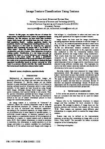
where Lθx indicates the derivative of image L(x) in orientation θ. To discriminate two or more textures, we use the additional information provided in different scales/derivatives to achieve a better performance (comparing to single scale). To this end, the patches are extracted from the textures in the original and derivative scale spaces. The size of the patch is scale dependent. As we go to higher scales, i.e. lower resolutions, more emphasis is given to coarser structures and (in similar fashion as our visual system) we need to look at these structures through larger windows. Thus, we increase the size of patches when we go to higher scales. These patches can be subsampled to reduce the computation load. The main goal in this multi-scale texture classification system is to identify to what extent the additional information provided by other scales/derivatives can improve the performance. Hence, the patches should be taken from the same spatial locations in the scale-space. This is shown graphically in Fig. 1 for one patch extracted from different scales/derivatives for a typical texture image. Higher Scales

(x0, y0)

(x0, y0)

y

(x0, y0)

x Fig. 1. Illustration of the method for selection of a typical patch from three different scales of the same texture. The patches are taken from the same spatial locations in different scales. However, the size of patch increases as we go to higher scales. The spatial location should be also the same in different derivatives of the same texture.

2.2 Feature Extraction The patch size affects the dimensionality of the feature space as larger patches generate more features. This may impose problems with respect to the computation speed and the necessary training set size. Increasing the feature space dimension usually degrades the performance of the classifier unless we dramatically increase the number of data samples for training (curse of dimensionality) and may cause the peaking phenomena in classifier design. There are two solutions to this problem: to increase the training set size, and to reduce the feature space dimension using feature selection/extraction techniques, e.g. Principal Component Analysis (PCA).

328

M.J. Gangeh, B.M. ter Haar Romeny, and C. Eswaran

2.3 Combined Classifier As mentioned in the introduction, the common practice in multiresolution texture classification is concatenating the features obtained from different resolutions to construct a combined feature space. This combined feature space is fed to a classifier. This produces a high dimensional feature space and therefore severe feature reduction is required using feature selection/extraction techniques. The alternative method proposed in this paper is using combined classifiers. Combined classifiers are used in multiple classifier source applications like different feature spaces, different training sets, different classifiers applied for example to the same feature space, and different parameter values for the classifiers, e.g. k in knearest neighbor (k-NN) classifiers. In this approach, the features obtained from each scale are applied to a base classifier. As the features spaces generated from different scales/derivatives are different in our method, parallel combined classifiers seem to be natural choice. Use of combined classifiers lifts the requirement for feature space fusion. Moreover, each base classifier can be examined separately, e.g. by drawing the corresponding learning curve, to determine the contribution of each scale/derivative towards the overall performance of the classification algorithm as will be shown in section 4. Here, we propose a two-stage parallel combined classifier with the structure shown in Fig. 2. As can be seen in this figure, in the first stage, the feature space from each scale/derivative is applied to a base classifier. At the output of this stage a fixed combining rule is applied to combine the outputs of different scales for one particular order of derivative. For example scales s1, s2 and s3 for the Lx are combined using a fixed combining rule. In the second stage, the outputs of the first stage, i.e. all different derivatives, are combined to produce the overall decision on the texture classes. First Stage S1

BC

S2

BC

Sn

M

Second Stage

CC 1

BC

S1

M

BC

M

S2

BC

CC k

Sn

M

BC

OCC Abbreviations: S: Scale BC: Base Classifier CC: Combining Classifier OCC: Overall Combining Classifier

Fig. 2. The structure of two-stage combined classifier proposed in this paper

This two-stage parallel combined classifier provides a versatile tool to examine the contribution of each derivative in the overall performance of the classifier. However, it must be noticed that if two combining rules are the same, e.g. if both are fixed

Scale-Space Texture Classification Using Combined Classifiers

329

‘mean combining’ rule, this two stage combined classifier is not different from one stage where all the feature spaces are applied to the base classifiers and the outputs are combined using the same combining rule. Two parameters have to be selected in this combined classifier: the type of the base classifier and the combining rule. The selection of these two options is discussed in section 4. 2.4 Evaluation One of the main shortcomings of the papers in multiresolution texture classification is reporting the performance of the algorithm for one single training set size. This causes that the behavior of the algorithm for different training set sizes remains unrevealed. In this paper, to overcome this problem and to investigate the performance of the classifier, the learning curves are drawn by calculating the error for different training set sizes. Since the train and test sets are generated from the same image in each scale/derivative, they may spatially overlap in the image domain. Hence, to assure that the train and test sets are separate, we split the texture images spatially into two halves and generate the train and test sets from each half. As we have constructed the train set and test sets from two different halves of the image we can use a fixed test set size for calculating the error of the combined classifier trained using different train set sizes. This may improve the accuracy of error computation as we can increase the test set size independent from the train set size at the cost of higher computational load.

3 Experiments To evaluate the effectiveness of the proposed method, some experiments are performed on a supervised classification of some test images. The test images are from the Brodatz album as shown in Fig. 3. Construction of Multi-scale Texture Images. The N-jet of scaled derivatives up to the second order is chosen to construct the multi-scale texture images from each texture. Based on steerability of Gaussian derivatives, we have used the zeroth order derivative, i.e. the Gaussian kernel itself, Lx, Ly, Lxx, Lxy, Lyy, and Lxx+ Lyy where the last one is the Laplacian. For each derivative (including the zeroth order) three scales are computed. The variances (σ2) of the Gaussian derivatives in scales s1, s2 and s3 are 1, 4 and 7 respectively. In this way, for each texture image 7×3 texture images are computed. Preprocessing. To make sure that for all textures the full dynamic range of the gray level is used contrast stretching is performed on all textures in different scales. Also, to make the textures indiscriminable to mean or variance of the gray level, DC cancellation and variance normalization are performed.

330

M.J. Gangeh, B.M. ter Haar Romeny, and C. Eswaran

Fig. 3. Textures D4, D9, D19 and D57 from Brodatz album used in the experiments

Construction of Train and Test Sets. To ensure that the train and test sets are completely separate, they are extracted from the upper and lower half of each image respectively. For one texture, the patches are with sizes of 18×18, 24×24, and 30×30 in scales s1, s2 and s3 respectively. For the time being no subsampling is performed in higher scales but this might be considered in future for optimization of the algorithm in terms of speed and memory usage. Test set size is fixed at 900. Train set size increases from 10 to 1500 to construct the learning curves. Feature Extraction. PCA is used for feature extraction. The number of components used for dimension reduction is chosen to preserve 95% of the original variance in the transformed (reduced) space. Combined Classifier. A two-stage parallel combined classifier is used. A variety of base classifiers and combining rules are tested to find the best one. Among the base classifiers tested are some normal-based density classifiers like quadratic discriminant classifier (qdc), linear discriminant classifier (ldc), and nearest mean classifier (nmc). The Parzen classifier was also tested as a representative of non-parametric based density classifier. Twenty one base classifiers, one for each scale in one derivative order are used. The mean, product and voting fixed combining rules as well as the nearest mean trainable combining rule are tested for comparison. Evaluation. The performance of the texture classification system is evaluated by drawing the learning curves for training set sizes up to 1500. The error is measured 5 times for each training set size and the results are averaged.

4 Results A variety of tests are performed using different parameters as explained in the previous section. Among the tested base classifiers qdc performed the best. This can be understood as PCA is a linear dimension reduction that performs integration in the feature space. Consequently, the features tend to be normally distributed based on the central limit theorem. Of the tested combining rules ‘mean combiner’ performs best. Hence, the results are shown here based on experiments using qdc as base classifier and mean combining rule for both stages. The left graph in Fig. 4 displays the learning curves obtained at the output of stage 1 (combined scales for each derivative order) and stage 2 (combine all derivatives in all scales) of the two-stage combined classifier. As can be seen, the overall performance of the classifier is improved comparing to each derivative order in different scales. This is especially significant in small training set sizes. However, for very

Scale-Space Texture Classification Using Combined Classifiers

331

small training set sizes, i.e. below 200, the output of the combined classifier is degraded significantly. This is because of peaking phenomena as the dimension of feature space in scale 1 is rather high even after applying PCA. Combined Classifier with Regularization of Base Classifiers in Scale 1. To overcome the size problem, we applied regularization to the qdc base classifier in scale 1 for all derivative orders (right graph in Fig. 4). The performance improved significantly in very small training set sizes, i.e. below 200. One of the major drawbacks of regularization is that it ruins the results for large training set sizes. However, as we have only applied the regularization to scale 1, the information from other scales prevents deteriorating the performance in large training set sizes as can be judged from the graph. Combined Classifier with the Same Patch Size in All Scales. The left graph in Fig. 5 illustrates the importance of increasing patch size in higher scales. In this figure, the patch sizes extracted from the multi-scale texture images in different scales are the same (18×18). It is apparent that the performance of the classifiers in higher scales is degraded compared to Fig. 4. Combined Feature Space versus Combined Classifier. To demonstrate the superiority of our method to the common trend in the literature on multiresolution texture classification, we compare the results of two classification tests: combining the features obtained from different scales in the zeroth order derivative with the case that we use a combined classifier for the same derivative order in different scales. The results are shown in the right graph of Fig. 5 and the superiority of using a combined classifier to combined feature space is obvious. Combining all features generated from different scales/derivatives produces very high dimensional feature space that leads to extremely poor performance in combined feature space technique. Hence, the comparison has been made in only one derivative order. It should be also highlighted here that combined classifier approach is computationally much less expensive than combined feature space technique as applying fused feature space to one base classifier needs huge amount of memory space simultaneously and runs slowly compared to the combined classifiers.

5 Discussion and Conclusion Scale-space theory, PCA and combined classifiers are integrated into a texture classification system. The algorithm is very efficient especially in small training set size. The system can significantly improve the performance of classification in comparison with single scale and/or to single derivative order based on the information provided in multiple scales and multiple derivative orders. The two-stage combined classifier along with the learning curves proposed in this paper provides a versatile means to investigate the significance of different scales/derivatives in overall performance of the classifier. Regularization of qdc base classifier in scale 1 further improves the performance especially in small and very small training set sizes. This, however, does not deteriorate the results in large

332

M.J. Gangeh, B.M. ter Haar Romeny, and C. Eswaran 0.8

0.8

Average error (5 experiments)

0.7 0.6 0.5 0.4 0.3 0.2

0.6 0.5 0.4 0.3 0.2 0.1

0.1 0 0

Combined Classifier Combined Gaussian Combined Lx Combined Ly Combined Lxx Combined Lxy Combined Lyy Combined Laplacian

0.7 Average error (5 experiments)

Combined Classifier Combined Gaussian Combined Lx Combined Ly Combined Lxx Combined Lxy Combined Lyy Combined Laplacian

250

500

750 1000 Training set size

1250

0 0

1500

250

500

750 1000 Training set size

1250

1500

Fig. 4. Learning curves for the classification of 4 textures from the Brodatz album at multiple scales of single and multiple derivative orders without regularization (left graph) and with regularization (right graph) of base classifiers at scale 1 0.8

0.8

Average error (5 experiments)

0.7 0.6 0.5 0.4 0.3 0.2

Combined Classifier Combined Feature Space

0.7 Average error (5 experiments)

Combined Classifier Combined Gaussian Combined Lx Combined Ly Combined Lxx Combined Lxy Combined Lyy Combined Laplacian

0.6 0.5 0.4 0.3 0.2

0.1 0 0

250

500

750 1000 Training set size

1250

1500

0.1 0

250

500

750 1000 Training set size

1250

1500

Fig. 5. Learning curves for the classification of 4 textures from the Brodatz album with regularization of base classifiers at scale 1 using the same patch size for all scales (Left graph). Learning curves obtained using the combined classifier and the combined feature space methods for the zeroth order derivative (Right graph).

training set sizes thanks to the information provided from other scales. This approach is superior to the combined feature space in terms of performance and computation load. This algorithm is effective in situations where gathering many data samples for the train/test sets is difficult, costly or impossible. E.g. in ultrasound tissue characterization image acquisition has to be standardized and the ground truth for diffused liver diseases is biopsy, which is invasive, and collection of data is very time consuming. In these situations this algorithm can improve the performance of the classification over classical approaches as the train set size is small. In future work, we want to apply this method to distinguish normal from abnormal lung tissue in high resolution CT chest scans.

Scale-Space Texture Classification Using Combined Classifiers

333

Acknowledgement. The authors would like to thank R.P.W. Duin from Delft University of Technology for useful discussions throughout this research.

References 1. Materka, A., Strzelecki, M.: Texture Analysis Methods-A Review. Technical University of Lodz, Institute of Electronics, COSTB 11 report, Brussels (1998) 2. Hadjidemetriou, E., Grossberg, M.D., Nayar, S.K.: Multiresolution Histograms and Their Use for Recognition. IEEE Trans. on PAMI 26, 831–847 (2004) 3. Andra, S., Wu, Y.J.: Multiresolution Histograms for SVM-Based Texture Classification. In: Kamel, M., Campilho, A. (eds.) ICIAR 2005. LNCS, vol. 3656, pp. 754–761. Springer, Heidelberg (2005) 4. van Ginneken, B., ter Haar Romeny, B.M.: Multi-scale Texture Classification from Generalized Locally Orderless Images. Pattern Recognition, Vol. 36 pp. 899–911 (2003) 5. Kang, Y., Morooka, K., Nagahashi, H.: Scale Invariant Texture Analysis Using MultiScale Local Autocorrelation Features. In: Kimmel, R., Sochen, N.A., Weickert, J. (eds.) Scale-Space 2005. LNCS, vol. 3459, pp. 363–373. Springer, Heidelberg (2005) 6. Ojala, T., Pietikainen, M., Maenpaa, T.: Multiresolution Gray-Scale and Rotation Invariant Texture Classification with Local Binary Patterns. IEEE Trans. on PAMI 24(7), 971–987 (2002) 7. Wang, L., Liu, J.: Texture Classification Using Multiresolution Markov Random Field Models. Pattern Recognition Letters 20, 171–182 (1999) 8. Randen, T., Husoy, J.H.: Filtering for Texture Classification: A Comparative Study. IEEE Trans. on PAMI 21, 291–310 (1999) 9. Li, S.T., Shawe-Taylor, J.: Comparison and Fusion of Multiresolution Features for Texture Classification. Pattern Recognition Letters 26, 633–638 (2005) 10. Jain, A.K., Farrokhnia, F.: Unsupervised Texture Segmentation Using Gabor Filters. Pattern Recognition 24, 1167–1186 (1991) 11. Kim, K.I., Jung, K., Park, S.H., Kim, H.J.: Support Vector Machines for Texture Classification. IEEE Trans. on PAMI 24(11), 1542–1550 (2000) 12. Haley, G.M., Manjunath, B.S.: Rotation-Invariant Texture Classification Using a Complete Space-Frequency Model. IEEE Trans. on Image Processing 8(2), 255–269 (1999) 13. Choi, H., Baraniuk, R.G.: Multi-scale Image Segmentation Using Wavelet-Domain Hidden Markov Models. IEEE Trans. on Image Processing 10(1), 1309–1321 (2001) 14. ter Haar Romeny, B.M.: Front-End Vision and Multi-scale Image Analysis: Multi-scale Computer Vision Theory and Applications (Written in Mathematica). Kluwer Academic Publishers, Dordrecht, the Netherlands (2003) 15. Jain, A.J., Duin, R.P.W., Mao, J.: Statistical Pattern Recognition: A Review. IEEE Trans. on PAMI 22(1), 4–37 (2000) 16. Kadah, Y.M., Farag, A., Zurad, J.M., Badawi, A.M., Youssef, A.B.M.: Classification Algorithms for Quantitative Tissue Characterization of Diffuse Liver Disease from Ultrasound Images. IEEE Trans. on Medical Imaging 15, 466–478 (1996)