A Two-Stage Combined Classifier in Scale Space Texture Classification

A Two-Stage Combined Classifier in Scale Space Texture Classification Mehrdad J. Gangeha,∗, Robert P.W. Duinb , Bart M. ter Haar Romenyc , Mohamed S. Kamela

arXiv:1207.4089v1 [cs.CV] 17 Jul 2012

a Center

for Pattern Analysis and Machine Intelligence, Department of Electrical and Computer Engineering, University of Waterloo, 200 University Avenue West, Waterloo, ONT. N2L 3G1, Canada b Pattern Recognition Laboratory, Delft University of Technology, Mekelweg 4, 2628 CD Delft, The Netherlands c Biomedical Image Analysis Group, Department of Biomedical Engineering, Eindhoven University of Technology, Den Dolech 2, NL-5600 MB Eindhoven, the Netherlands

Abstract Textures often show multiscale properties and hence multiscale techniques are considered useful for texture analysis. Scale-space theory as a biologically motivated approach may be used to construct multiscale textures. In this paper various ways are studied to combine features on different scales for texture classification of small image patches. We use the N-jet of derivatives up to the second order at different scales to generate distinct pattern representations (DPR) of feature subsets. Each feature subset in the DPR is given to a base classifier (BC) of a two-stage combined classifier. The decisions made by these BCs are combined in two stages over scales and derivatives. Various combining systems and their significances and differences are discussed. The learning curves are used to evaluate the performances. We found for small sample sizes combining classifiers performs significantly better than combining feature spaces (CFS). It is also shown that combining classifiers performs better than the support vector machine on CFS in multiscale texture classification. Keywords: classifier design and evaluation, scale space, multiresolution, multiple classifier systems, texture

1. Introduction There is a vast literature on texture analysis, as can be judged from its numerous applications in various fields [1]. Texture analysis has been applied to nine broad categories [1–7]: ∗ Corresponding

author Email addresses: [email protected] (Mehrdad J. Gangeh), [email protected] (Robert P.W. Duin), [email protected] (Bart M. ter Haar Romeny), [email protected] (Mohamed S. Kamel) Preprint submitted to Elsevier

July 18, 2012

1. Texture classification of stationary texture images that contain only one texture type per image. 2. Unsupervised texture segmentation of nonstationary images that consist of more than one texture type per image. 3. Texture synthesis, which is important in computer graphics for rendering object surfaces to be as realistic looking as possible. 4. 3D shape from texture, which investigates how a standard texel shape is distorted by 3D projections and relates it to the local surface orientation. 5. Shape from texture, in which texture is usually used in addition to other features such as shading, color, and so on to extract three-dimensional shape information. 6. Color-texture analysis, where joint color-texture descriptor improves discrimination over using color and texture features independently. 7. Texture for appearance modeling, which is fundamental in computer vision and graphics. 8. Dynamic texture analysis for dynamic shape and appearance modeling which is essential in video sequences with certain temporal regularity properties. 9. Indexing and image database retrieval usually based on similarity measure. In this paper, the focus is on texture classification among the texture analysis problems and hence in the remaining of the text, all the examples and statements are for this problem. As texture is a complicated phenomenon, there is no unique definition that is agreed upon by the researchers [8]. However, for the purpose of this paper, we adopt to the definition provided in [5]: “Texture is the variation of data at scales smaller than the scales of interest”. Textures often show multiscale/multiresolution properties. This means that information from other scales can help to perform a more accurate texture analysis or, for example in texture classification, enables to train the classifier(s) by a smaller training set. This inspires the use of multiresolution techniques in texture analysis. 1.1. Studies on Multiresolution Texture Analysis Multiresolution techniques in texture analysis can be divided into two broad categories: techniques based on a single approach and those which are based on a combination of approaches. Some of the most well-known multiresolution techniques on texture analysis in the former category given above are: multiresolution histograms [2, 9] including locally orderless images [10], techniques based on multiscale local autocorrelation features [11], multiresolution local binary patterns [12, 13], multiresolution Markov random fields [14– 17], wavelets [4, 18–22], Gabor filters [19, 23, 24], multiscale tensor voting [25], a technique based on multiresolution fractal feature vectors [26], and techniques based on scale-space theory [10, 27–29]. In these approaches, feature subsets from different scales are fused to construct a single feature space. This space is then submitted to a single classifier. These approaches report better results than those based on a single resolution. Two research works in the literature that report fusion of two or more multiresolution techniques are: fusion of dyadic wavelet transform, steerable pyramid, Gabor wavelet transform, and wavelet frame transform in [30], and combining Laws filters, Gabor, and wavelets in [31]. These papers also report better results than single multiscale techniques. 2

1.2. Contributions The main issue in multiresolution techniques is the large feature space generated. The common trend in the literature, which is the fusion of the feature subsets generated at different scales to come up with one feature space to be submitted to a classifier, makes the problem even more serious. The large feature space, however, suffers from the ‘curse of dimensionality’ [32]. To tackle this problem typically severe feature reduction is applied in multiresolution techniques, e.g. by using histogram moments [10, 27, 28], calculating the energy [19], or maximum entropy [17]. However, the performance of the classifiers trained for such a reduced feature space highly depends on how well these features represent the data in the particular application. This problem is also addressed in the literature by using classifiers that behave better in high dimensional feature space, e.g., support vector machines (SVMs) [9, 24]. Also, the multiresolution papers in texture classification only report the classification error for a single specific (usually large) training set size. This keeps the behavior of the classifier unrevealed in small training set sizes that might be important in some applications especially those where obtaining a large training set size is difficult, costly or even impossible. This is particularly the case in texture classification applications on medical images: obtaining medical images for some specific diseases is cumbersome especially in the case that standardized protocols for image acquisition are difficult to be followed, such as in ultrasound images [33]. This paper addresses the following two issues. First, we use combined classifiers instead of fusing feature subsets. In combined classifiers, feature subsets produced at various scales are submitted to base classifiers and hence feature fusion is no longer required. Next, the outputs of these base classifiers are combined for a final decision on the class of each texture. We propose a two-stage structure for this purpose and discuss the benefits obtained. We also provide the mathematical formulation for the proposed two-stage combined classifiers and its relation to one-stage structure. Second, the learning curves for training the classifiers are constructed for different training set sizes. This clearly shows how the training of the classifier evolves as we increase the training set size. Our focus is on the classification of small patches, which is a more challenging task as the information contained is less than large ones. Our results lead to an important conclusion: convolution with filters like wavelets, Gabor, and Gaussian derivatives, which are used for the construction of feature subsets at different scales/resolutions, consists of linear operations. If there are no zero-weights, no information is lost as they are invertible. All information is available in the original space, i.e., at highest resolution and can be used for classification provided that the set of training samples is sufficiently large. As this is usually not possible or prohibitive, the information from other scales is provided to train the classifier using fewer data samples. 1.3. Previous Work on Combined Classifiers in Multiresolution Texture Analysis A few papers in the literature examine the application of multiple classifier systems (MCS) in multiresolution texture classification. The application of MCS in multiresolution texture classification using SVMs as base classifiers (BCs) and wavelets as the multiresolution technique is investigated in [34]. The SVMs use different kernels. Combining them by majority voting produced better results than a single SVM if applied to the Brodatz album. Also [35] addresses the classification of multispectral images with 3

the application in remote sensing using ensemble of classifiers with SVMs as the base classifiers. The results show improvement over single SVM. On the other hand, it is reported in [36] that using combined classifiers to combine three different multiresolution techniques, i.e., Gabor, wavelets and the combination of these two using k -NN or SVMs as base classifier does not improve over the best single classifier for scenery images. However, to our best of knowledge, there is no work in the literature on using combined classifiers where the feature subsets from different scales are submitted to the BCs. In this paper, we will discuss this approach and the benefits obtained. Scale space theory in the context of multiscale texture classification is presented in Section 2. In Section 3, combined classifiers and their application in scale space texture classification are explained. The experiments are elaborated in Section 4 followed by the results in Section 5. The comparison between the proposed approach and other techniques is presented in Section 6. Eventually, the effectiveness of the method, especially for small training set sizes, is discussed in Section 7. 2. Scale Space Texture Classification A texture classification system typically consists of several stages like preprocessing, feature extraction, and classification, which are discussed in this and next sections. 2.1. Construction of Multiscale Textures In the recent years, multiresolution techniques gained importance in texture analysis due to the intrinsic multiscale nature of textures. Among the multiscale techniques in the literature summarized in Section 1.1, the techniques based on scale space theory provide a mathematical framework for texture analysis which is biologically motivated by the models of the early stages of human vision [29]. We express the theory of scale space in the context of texture classification as follows: We assume here that we only deal with gray scale textures. A texture can be considered as a function Li that maps the spatial information into intensity levels, i.e., Li : Z2 → Z,

i = 1, ..., c

(1)

where c is the number of textures (classes) to be classified. Spatial information and intensity are both assumed to be quantized1 . According to scale space theory [29], to extract the multiscale differential texture structure ∂ n Li (x; σ)/∂xn , i = 1, ..., c, n ≥ 0, where σ is the scale, we need to calculate the derivative of the observed image by a Gaussian aperture: ∂n ∂n L (x; σ) = (Li ∗ Gσ )(x), i ∂xn ∂xn

(2)

1 In fact, the formulation provided for scale space can be applied to continuous images as well. However, the digital images are always quantized in both spatial and intensity spaces and hence we have assumed this as a realistic situation. Scale space addresses taking the derivative of discrete data (like digital images) by applying regularization on the image (by convolving image with a Gaussian kernel). This is usually addressed in the field of image processing by approximating differentiation by differencing which is avoided here.

4

where ∗ is the convolution operator and Gσ is the 2D Gaussian kernel at scale σ Gσ (x) =

1 − x22 e 2σ . 2πσ 2

(3)

Since both convolution and differentiation are linear operators in (2), they can be commuted ∂n ∂n Li (x; σ) = (Li ∗ Gσ )(x), (4) n ∂x ∂xn which means that to obtain the multiscale textures ∂ n Li (x; σ)/∂xn , i = 1, ..., c, n ≥ 0, one needs to convolve the original textures Li (x), i = 1, ..., c, with the derivatives of the Gaussian kernel at multiple scales (n = 0 is for the convolution with the Gaussian kernel, i.e., for the zeroth order derivative). The order of the derivatives determines the type of structure to be emphasized. For example, the first order derivative extracts the edges, the second order emphasizes on the ridges and corners and so on. The order of the derivatives used to construct the multiscale textures might be application dependent. To avoid excessive computational load typically up to the second order derivatives are used. To address the issue of the number of orientations required in each derivative order, we use the steerability property of Gaussian derivatives [29, 37] for the efficient computation of directional derivatives. Based on this property, in the n th order derivative, n + 1 independent orientations are needed with which the derivatives in any orientation (in the same order) can be calculated. For example, for the first order derivative, i.e., n = 1, the derivative in arbitrary orientation θ can be calculated using Lx and Ly : Lθ (x, y) = cos(θ) × Lx (x, y) + sin(θ) × Ly (x, y),

(5)

where Lθ is the derivative of L(x) in orientation θ. As a general setup is considered in this research, the formulation provided in (4) is sensitive to orientation transformations. If rotation invariance is desired in an application, differential invariant descriptors, which are directly derived from combination of components of the local jet in scale space theory, can be adopted [38]. 2.2. Construction of Multiscale Feature Spaces To construct the multiscale feature space out of the multiscale textures, features are extracted from each scale to generate n-dimensional vectors v(i) = [v1 , ..., vn ] ∈ Rn , i = 1, ..., ns×nd, where nd is the number of derivatives and ns is the number of scales in each derivative. This generates m = ns × nd feature subsets at different scales/derivatives. Although this generation of feature subsets discussed in the context of construction of multiscale textures using scale space theory, it can be easily extended to other multiresolution techniques where m feature subsets are generated at various resolutions. In other multiresolution techniques, m also could be a multiplication of two other parameters, e.g., using Gabor kernels, the multiresolution textures are obtained by varying the center frequency in each band and the scale. Hence, m will be the multiplication of the number of central frequencies and the number of scales. In this paper, however, we restrict ourselves to Gaussian derivatives for the generation of feature subsets. These feature subsets can be composed into a single feature vector v = [v(1) , v(2) , ..., v(m) ]> , which is called the distinct pattern representation (DPR) [39]. The dimensionality of the 5

various feature subsets x(i), i = 1, ..., m, is not necessarily the same. As we will discuss later in Section 2.5, fewer features will be extracted from higher scales due to the coarser structures or less information available at these scales. 2.3. Combined Classifiers versus Combined Feature Spaces After extraction of feature subsets v(i) = [v1 , ..., vn ]> ∈ Rn , i = 1, ..., m, from all scales, the common trend in the literature is to concatenate these feature subsets to build up a single feature space v ∈ Rn×m , called combined feature space (CFS) in this paper, where n is the dimensionality of each feature subset and m is the total number of feature subsets. The dimensionality of different feature subsets (n) might not be necessarily the same. However, for the time being and for the simplicity of the discussion, we assume that all feature subsets have the same dimensionality. The obtained fused feature space is then submitted to a single classifier D : Rn×m → Ω, where Ω = {ω1 , ..., ωc } is the set of class labels for the textures. The main disadvantage of this approach is that the fusion of feature subsets generates a high dimensional feature space that may cause suffering from the ‘curse of dimensionality’ [32]. This can be solved in three ways: 1. By reducing the dimensionality of each feature subset significantly. This can be done by a general procedure like principal component analysis (PCA), derived from the data, or based on the specific nature of the features. For example, in filter bank approaches like Gabor or wavelets, the outputs are not directly used. The features are produced by taking the local standard deviation, or the local energy, i.e., by a kind of energy estimate for each local window/patch extracted around each pixel [5, 19]. Some researchers calculate the moments of histogram on patches or regions of interest (ROIs) extracted from multiscale textures [10, 27, 28]. 2. By using classifiers that behave well in high dimensional feature spaces like support vector machines (SVMs) [9, 24] a significant feature reduction in each scale is not needed. 3. By submitting the DPR to an ensemble of classifiers ℘ = {D1 , ..., Dm },

℘ : Rn×m → Ωm ,

(6)

where Di : Rn → Ω, i = 1, ..., m, is the base classifier trained on each feature subset v(i) ∈ Rn , i = 1, ..., m. Then the decisions made by these BCs are fused. Thus, the problem of finding a classifier D : Rn → Ω is converted into finding an aggregation method = : Ωm → Ω for combining the classifier outputs. Our focus is on the third approach where we construct a two-stage combined classifier in the scale space texture classification context. We, thereby, emphasize more on the classifier structure than on the multiresolution technique. 2.4. The Construction of DPR for the Ensemble of Classifiers In the above methods, the features are usually calculated on local windows/patches around pixels extracted from the constructed multiscale textures. To reduce the dimensionality of the feature space in the CFS approach, usually the energy of output filters, the moments of histograms, or other measurable parameters are calculated from these local patches and are considered as the feature subset v(i) , i = 1, ..., m for a particular 6

scale. These feature subsets are then concatenated to construct the fused feature space v to be submitted to a single classifier. In the proposed approach using combined classifiers, the feature space obtained from each scale is submitted to a BC. Instead of fusion of features from different scales, the decisions made by the BCs are combined. Thus, a severe feature reduction is not required. Hence, in this approach, to construct the multiscale feature space (or the DPR), the pixels from the extracted patches in each scale can be used to construct the feature subsets in that scale. This means that each feature subset from each scale is constructed using the pixels in a patch extracted from this scale. As many patches as necessary are extracted to construct the training and test sets. The dimensionality of this feature subset (n) depends on the number of pixels in the patch, i.e., patch size. To address the issue related to how to extract the patches from different scales we notice that the patch size is scale dependent and at higher scales (lower resolutions), the patch size should be increased. This is mainly because as we go to higher scales, more emphasis is given on coarser structures and hence they should be looked at through larger windows. On the other hand, the patches from different scales/derivatives of the same texture must be extracted from the same spatial locations to identify to what extent the additional information provided by other scales/derivatives can improve the performance of the classification system. 2.5. Subsampling and Feature Reduction As explained above, at higher scales, the patch sizes should be increased to represent the coarser structures available at these scales. To overcome the resulting problem of large memory storage and high computational costs, subsampling can be performed at higher scales. In [40], it is shown that subsampling will not degrade the performance of the multiscale texture classification system while it can reduce the required memory space and computational cost. To reduce the dimensionality of feature subsets further, feature extraction/selection techniques can be deployed, such as principal component analysis (PCA) or independent component analysis (ICA) [41]. While PCA is the most prevalent feature extraction method in the literature, there have recently been several works published to compare PCA and ICA as the feature extraction techniques in object recognition with some contradictory results (refer to [42] for a list). In Chapter 7 of [43], it is concluded that it is very difficult to find the independent components in a very high dimensional feature space and it usually leads to no significant improvement over PCA. In [42], it is shown how PCA and ICA are related as the feature extraction techniques and under which conditions their performance is completely equivalent. There are several suggestions to get better performance by ICA than by PCA where using feature selection (a subset of the original feature space to avoid searching in a very high dimensional feature space, which is consistent with the conclusion in [43]) is one main possibility [42]. Considering the simplicity of PCA in comparison to ICA and to avoid an extra feature selection step, which is not very obvious in our task, PCA is adopted in this research for feature extraction. Its application to scale space texture classification using combined classifiers is discussed in [40, 44]. PCA performs an adaptive feature extraction in multiscale texture classification in this sense that at higher scales the size of the patches need to be increased and hence more dimension reduction is required. PCA adapts itself according 7

GANGEH ET AL.: A TWO-STAGE COMBINED CLASSIFIER IN SCALE SPACE TEXTURE CLASSIFICATION

5

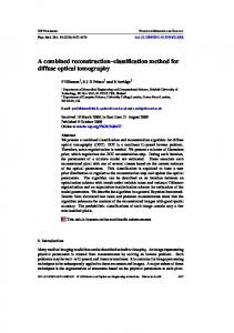
t is very difficult to find the independent components in BC FR S1 a very high dimensional feature space and it usually leads o no significant improvement over PCA. In [58], it is FR BC S 2 L shown how PCA and ICA are related as the feature ex  raction technique and under which conditions their perFR BC Sns ormance is completely equivalent. There are several suggestions to get better performance by ICA than by PCA S1 BC FR where using feature selection (a subset of the original feaBC FR S2 ure space to avoid searching in a very high dimensional Lx eature space, which is consistent with the conclusion in   BC FR Sns 10]) is one main possibility [58]. Considering the simplicty of PCA in comparison to ICA and to avoid an extra  eature selection step, which is not very obvious in our Abbreviations: S1 FR BC ask, PCA is adopted in this research for feature extracS: Scale ion. Its application to scale space texture classification S2 FR BC FR: Feature Reduction Lyy using combined classifiers is discussed in [16] and [19]. BC: Base Classifier   PCA can perform an adaptive feature extraction in mulSns FR BC : Combiner iscale texture classification in this sense that for higher scales the sizes of the patches need to be increased and Fig. 1. The structure of multiscale texture classification using onestage combined classifier proposed in thisclassification paper. hence more dimension reductionFigure is required. 1: PCA Theadapts structure of multiscale texture using one-stage combined tself according to scale as there are fewer details at highclassifier proposed in this paper. for the decisions made by the BCs, and er scales and thus fewer components are needed to main4. feature level, different feature subsets might be ain the same fraction of variance of the original space. applied to the BCs and the ensemble. By applying subsampling and PCA, the feature subsets For the second level of design, i.e., the classifier level, a (i) v , i = 1,…, m are mapped to anto uncorrelated space. This scale as there are fewer details at higher scales and thus fewer components are needed builds up new feature subsets u(i), i = 1,…, m by which a variety of parametric classifiers, e.g., the linear discrimifraction of variance of quadratic the original space.clasclassifier (LDC) and the discriminant (1) (2) ( m ) Tto maintain the same nant new DPR u [u , u , , u ] can be constructed. The (i) the sifier (QDC), as PCA, well as nonparametric Bymight applying subsampling and the feature classifiers, subsetsve.g., , i = 1, ..., m are mapped dimensionalities of new feature subsets be different k nearest neighbor (k-NN) and Parzen classifiers are exrom each other and depend ontotheannumber of compo- space. This builds up new feature subsets uncorrelated u(i) , i = 1, ..., m, which QDC nents needed by PCA to retain specific fraction of va- amined (1) among (2) which(m) > performed the best and hence yields a new DPR u = [u , u , ..., u ] . The dimensionalities of new feature subsets iance of the original space. The dimensionality of feature selected as the BC. this other paper, our is mainly andcomponents needed by might belower different each andfocus depend on on thecombination number of subsets at coarser scales is usually much than atfrom In levels.ofInvariance feature level, the feature sub-The dimensionality of iner scales [16], [19]. PCA to retain specificfeature fraction of although the original space. sets are always generated using multiscale differential Fig. 1 shows the overall structure of the scale spaceat texfeature subsets coarser scales is usually much lower than the finer scales [40]. ure classification system using combined classifiers de- operators to construct multiscale textures, different comFig. 1 shows the overall structure of the scaleare space texture classification system using binations of the feature subsets mainly investigated. signed so far. This is somewhat combined classifiers designed so far. different from the combination level, where our focus is on the type of combiner for the out3 COMBINED CLASSIFIERS IN THE CONTEXT OF puts of the classifier ensemble. These two different levels MULTISCALE TEXTURE CLASSIFICATION are discussed in the next subsections in more details.

3. Combined Classifiers in the Context of Multiscale Texture Classification

As described in the previous section, instead of fusion of 3.1 Combination Level - The Type of Combiner eature subsets obtained from different Eachprevious base classifier Di, i = instead 1,…, m, inof thefusion ensemble geAs described in the section, of feature subsets obtained scales/derivatives, it seems to be natural to submit each T nerates a c-dimensional vector . Two types [ d , , d ] i ,1 i , c different it seems to be natural to 2submitofeach feature subset to eature subset to one classifier from and combine theirscales/derivatives, decioutputs are produced by the classifier ensemble : sions. There are several reasonsone given in the literature classifier and combine decisions. 1. their Class labels. In this case, we can assume that the why an ensemble of classifiers may perform better than a The types of combined classifiers are: which is used in applications with the output of each basestacked, classifier D m, in the i, i = 1,…, single classifier. They can be summarized as statistical, ensemble generates ain c-dimensional binary vecsame feature space; parallel, with application different feature spaces; and sequential, computational and representational reasons [31]. tor [d , , di ,c ]T {0,1}c , where di, j = 1 if Di labels The types of combined classifiers are: the stacked, which is are appliedi ,1 sequentially where classifiers one after another. As the features subsets u in class ωj, and 0 otherwise. used in applications with the same feature space; parallel, generated from different2.scales/derivatives are different in our method, parallel combined Continuous values, i.e., each base classifier Di, i = with application in different feature spaces; and sequential, 1,…, m,choice. in the ensemble generates a cclassifiers seem to be the natural where the classifiers are applied sequentially one after vector [di ,1 , , di ,c ]T [0,1]c , where another. As the features subsets generated Therefrom aredifferent four levels of dimensional design related to the construction of the classifier ensembles each di, j represents the support for the hypothesis scales/derivatives are different [45], in ouri.e., method, data parallel level : different datasets to train theforBCs; classifier level : the different BCs that the DPR u submitted classification to the combined classifiers seem to be the natural choice. classifier ensemble belongs to the ω j, j = 1,…, c.for the decisions made in the ensemble; combination level : the construction of combiners There are four levels of design related to the construcThis can be, for example, the posterior probability byi.e., the BCs; and feature level : different feature subsets might be applied to the BCs and ion of the classifier ensembles [31], p(ωj|u). In this way, the whole classifier ensemble 1. data level, different datasets train the BCs,In this paper, our focus is mainly on combination and feature levels. theto ensemble. generates a matrix of di, j, i = 1,…, m, and j = 1,…, c, 2. classifier level, the different BCs in the ensemble For the second level of design, i.e., the classifier level, a variety of parametric classifiers, 3. combination level, the construction of combiners

2 PRTools is used for the Matlab implementation of the algorithms [11]. e.g., the linear discriminant classifier (LDC) and the quadratic discriminant classifier

8

(QDC), as well as nonparametric classifiers, e.g., the k nearest neighbor (k -NN) and Parzen classifiers are examined among which QDC performed the best and hence selected as the BC. In this paper, our focus is mainly on combination and feature levels. In feature level, although the feature subsets are always generated using multiscale differential operators to construct multiscale textures, different combinations of the feature subsets are mainly investigated. This is different from the combination level, where our focus is on the type of combiner for the outputs of the classifier ensemble. These two different levels are discussed in the next subsections in more details. 3.1. Combination Level - The Type of Combiner Each base classifier Di , i = 1, ..., m, in the ensemble ℘ generates a c-dimensional vector [di,1 , ..., di,c ]> . Two types of outputs are produced by the classifier ensemble2 : 1. Class labels. In this case, we can assume that the output of each base classifier Di , i = 1, ..., m, in the ensemble ℘ generates a c-dimensional binary vector [di,1 , ..., di,c ]> ∈ {0, 1}c , where di,j = 1 if Di labels u in class ωj , and 0 otherwise. 2. Continuous values, i.e., each base classifier Di , i = 1, ..., m, in the ensemble ℘ generates a c-dimensional vector [di,1 , ..., di,c ]> ∈ [0, 1]c , where each di,j represents the support for the hypothesis that the DPR u submitted for classification to the classifier ensemble belongs to the ωj , j = 1, ..., c. This can be, for example, the posterior probability p(ωj |u). In this way, the whole classifier ensemble generates a matrix of di,j , i = 1, ..., m, and j = 1, ..., c, which is called a decision profile DP(u) [45]:   d1,1 · · · d1,j · · · d1,c  .. .. ..  .. ..  . . . . .     DP(u) =  di,1 · · · di,j · · · di,c  (7)   . .. ..  . . . . .  . . . . .  dm,1 · · · dm,j · · · dm,c where the elements di,j of matrix DP(u) are also dependent on u. However, this dependency is not shown in (7) and in the text for the simplicity of notation. In (7), each row is the output of classifier Di (u) and each column is the support from BCs, Di , i = 1, ..., m, for class ωj . The main goal at the combination level is to design an aggregation function = to combine the decisions at the output of BCs into a single decision. The design of = depends on the type of the outputs of BCs. 3.1.1. Combiners Based on the Class Labels Here, the aggregation function = selects the overall class label of the ensemble δ℘ (u) based on the class labels generated at the output of each BC in the ensemble. The most common combiner based on class labels is majority voting. This combiner considers the 2 PRTools

is used for the Matlab implementation of the algorithms [46].

9

output of the ensemble as the class label appeared at the output of the BCs more than others: m X c δ℘ = {δk |k = arg max di,j }. (8) j=1

i=1

3.1.2. Combiners Based on the Continuous Outputs The first step to use the continuous valued outputs of the BCs (e.g. confidences) is to make sure that they are normalized so all the outputs have equal contribution towards the overall performance of the system. Consequently, the confidences are summed to one at the outputs of the base classifiers and can be considered as posterior probabilities. In other words, the sum of the elements on each row of DP(u) matrix is one after normalization. This, however, does not alter the class membership of the data samples submitted for classification in the maximum a posteriori (MAP) probability sense. Here, we assume that di,j values of DP(u) matrix given in (7) are normalized. Combiners based on continuous valued outputs of the BCs are divided into two groups: nontrainable and trainable combiners. In nontrainable combiners, the aggregation function = calculates the support for the hypothesis that the submitted DPR u belongs to class ωj , using only the j th column of DP(u) by µj (u) = =(d1,j , ..., dm,j ). (9) There is no additional parameter to train. As soon as the outputs of the BCs are available, the overall output of the combined classifier can be calculated. The most common nontrainable combiners are: m

min combiner prod combiner

: µj (u) = min di,j i=1 Q m : µj (u) = i=1 di,j m

median combiner mean combiner max combiner

: µj (u) = median di,j i=1 Pm 1 : µj (u) = m i=1 di,j m : µj (u) = max di,j

(10)

i=1

Among these combiners, the min combiner selects the class to which all classifiers object the least. It is thereby careful and not sensitive for possible overtrained classifiers. The max combiner selects the class chosen by the most confident classifier. This is good if all classifiers are well trained and none of them is overtrained. The other combiners are between these two extremes. The mean and product combiners are the most common ones in the literature and their properties have been more investigated. While it is still not clear which combiner is the best, the results from other researches show that mean and product combiner may perform well in many applications [45]. However, according to experiments done by Kittler et al. [39], the mean combiner is more resilient to noise than the product combiner. Among trainable combiners, decision templates (DTs) are the simplest one. The DT can be calculated by averaging the DP(u) for the whole DPR. Then by calculating the decision profile for a test object and finding the nearest distance from the DT to this DP, the class label for the test object can be decided. 10

3.2. Feature Level - Combining of Feature Subsets In the construction of multiscale textures, different scales and different derivatives are used and hence, the feature subsets in DPR come from different scales of different derivatives. Each feature subset u(i) is submitted to one BC. Combining the BCs can be done in two ways: by combining all of them in one stage, as already explained and illustrated in Fig. 1; and by combining in two stages. In the latter case, there are several ways of combining. However, two straightforward methods of combinations are: 1. Different scales of the same derivative in the first stage and different derivatives in the second. 2. Different derivatives at the same scale in the first stage and different scales in the second. It is also possible to combine different scales of different derivatives in various ways. However, the above methods of combining group the feature subsets in a natural way, i.e., different derivatives of the same scale or different scales of the same derivative. Since the paper is about multiscale texture classification, in presenting the results, we focus more on combining different derivatives of the same scale to better realize the contribution of different scales towards the overall performance of the system. Moreover, it is also possible that a technique between combined classifiers and CFS is used: Concatenation of feature subsets in the first stage, then submitting them to the BCs and combining their decisions in the second stage. There are again various ways of combination. However, two more natural possibilities are: 1. Fuse feature combine the 2. Fuse feature combine the

subsets from different scales of the same derivative in the first stage and decisions made by the BCs in the second stage, or subsets from different derivatives at the same scale in the first stage and decisions made by the BCs in the second stage.

The architectures of two-stage scale space texture classification using combined classifiers for each of the above combinations are shown in Fig. 2. 3.2.1. A Two-Stage Combiner: Different Scales in the First Stage and Derivatives in the Second First we show the formulation for the two-stage combined classifier shown in Fig. 2a, i.e., combining the outputs of BCs for different scales of the same derivative in the first stage and then different derivatives in the second stage. The starting point is the matrix DP(u) in (7). However, we need to rearrange it as shown in Fig. 3a, where ns is the number of scales and nd is the number of derivatives. The decision profile DP(u) in Fig. 3a is subdivided into some submatrices by the dashed lines. Each submatrix is generated from the outputs of the same derivative at different scales in the first stage of the classifier ensemble (see Fig. 2a). Two aggregation functions are needed here. One aggregation function = to combine the elements of one column in each submatrix and the second one ϕ to combine all submatrices, i.e., µj (u) = ϕ[=(dj0 ), =(dj1 ), ..., =(djnd−1 )], (11) 11


9


9

GANGEH ET AL.: A TWO-STAGE COMBINED CLASSIFIER IN Stage SCALE SPACE TEXTURE CLASSIFICATION First Stage First Stage Second

Second Stage

First Stage First Stage BC Second Stage L BC FR FR GANGEHS1ET AL.: First A TWO-STAGE IN SCALE SPACE TEXTURE L Lx CLASSIFICATION BC BC BC COMBINED CLASSIFIER FR FR Stage First Second Stage FR BC FRStage S2 L S1 L BC FR BC L S1 S1S2 Lx BC BC FR FRFR Lyy First Sns FR BCStage BC FR First Stage Second Stage Lyy x FRFR BC FR S2Sns FR BC BC L S1 S1 L BC BC FR FR L BC S1 FR BC FR LxL L Sns yy BC FRFR 2 LS1 SFR S1 FR BC BC BC BC FR FRBC L FR BC S2 Lx S2 LyyLx x FRFRFR BCBC BC ns FR FR BC BC Lx S1S2 SFR S 2 L BC FR BC Lyy FR Sns BC BC FR FR BC BC x LLyy BC BC FRFR S2Sns SFR 1 FR FRBC Lx S2 L

Snsx S1S

1

LyyLyy Lyy

S2S2 S1 S S2nsSns Lyy

Sns

BC BC FR BC FR  BC 

S2

FR FR

FR

BC

Sns FR FR BC BC

BC FR S1 FR BC BC FR BC FR BC FR BC FR S2 (a) (a) BC FR Sns BC FR (a)

  

L L

S2S2 S1

L

Sns SLns 2

Lx

SSns1S1 S2 SSL12x Sns 2 Sns

SnsSns

Sns

Sns

Lx

Lx

Sns S1 S1 S2 Lyy SS12 Sns S2 S ns

Second Stage

 BC BCBC      

FR

BC

FR

FRFR

BC

FR

BC

Lx

FRFR BC BC BC FR FR FR BC FR BC BC FR BC

LLyyyy

FRFR

LL

Second Stage Second Stage

BC BC

(b) (b)

(b)

Second StageStage Second

BC

S1S1

L L x Lx

L

FR

LL x yy

Lx Lyy

FRFR

Lyy

FR

S2

BC

BC

S2

BC

 FR   FR   S FR FR FR  BCBC FF S FR FF

FR

FR First Stage First Stage

S1

S1

S2

S2

9

Second Stage

First Stage First Stage (b) (b)

FR

FR FR FR S1 FR FR FF FR FF FR S2 FR FF FR FR SnsFR FR FF

FR

L

Lx Lx L L Lyy L Lyy x

Second SecondStage Stage

FR FR First Stage First Stage FR FF BC S1 FR FR FF BC FR S2 FR FR FF BC FR FR FF BC

Sns

Lyy

LyyL

FirstStage Stage(a) (a) First

S1S1

Lx

S2

9

Second Stage

S1

FRFR FR

SecondSecond Stage Stage

FF FF

FR FR FF FF

BC

BC BC

BC

FR LLyy L FR FR LLx FRFR FF BC L x FR FF BC LLx FRFR FF BC Lyy FR L FF BC Lyyx Lyy FRFR FR

Lyy L

 

  

FR Abbreviations: FR Abbreviations: Abbreviations: S: Scale FR Lx S: Scale FR 2 FF BC S ns L S: ScaleReduction x FR Lyy FR: Feature FR BC FF Sns FR BC Abbreviations: FR: Feature Reduction L Lx FR FR FF FF BC FR FR S ns FR: Feature Reduction BC: Base Classifier Sns yy S: Scale BC: Base Classifier LL Lyy FRFR FR FF BC FR Lyyx FR FR FF: Features FF BC: BaseFusion Classifier BC S L ns yy FF: Features Fusion (c) (c) FR: Feature Reduction FR and :Classifier Combiners Sns Fusion andBC: : FF: Combiners BaseFeatures (c) Lyy FR and Fusion : Combiners FF: Features (c) Fig. 2. The structure of multiscale texture classification using two-stage combined classifier proposed in this paper with (a) combining differ(c)texture classification using two-stage combined classifier proposed (d) in this paper with Fig. 2. The structure of multiscale (a): Combiners combining differand ent scales the same derivative in the first stageand and different different derivatives second stage, (b) combining different derivatives at the at the ent scales of theofsame derivative in the first stage derivativesininthe the second stage, (b) combining different derivatives Fig.same 2. The structure of stage multiscale texture classification using stage, two-stage combined classifier proposed thisdifferent paper (a)same combining same scale the first stage different scalesininthe thesecond second stage, (c) ofof feature subsets obtained frominfrom different scaleswith of the scale in theinfirst andand different scales (c)fusion fusion feature subsets obtained scales of the same differderivative insame the first stage andin combining BCs in the second stage,derivatives and (d) fusion of feature subsets obtained from different derivatives at ent scales of the derivative the first stage and different in the second stage, (b) combining different derivatives derivative in thescale firstof stage and combining BCs inBCs theinsecond stage, and (d) fusion of feature subsetsinobtained fromwith different derivatives at at the Fig. 2. The structure multiscale texture classification using two-stage combined classifier proposed this paper (a) combining differthe same in the first stage and combining the second stage. same scale inthe thein first and and different scales inand the second stage, featurestage, subsets from different scales ofatthe sameof scale thestage first stage combining BCs in the second stage.(c) fusion entthe scales same derivative in the first stage different derivatives in theofsecond (b)obtained combining different derivatives thesame derivative in the first stage and combining BCs in the second stage, and (d) fusion of feature subsets obtained from different derivatives same scale in the first stage and different scales in the second stage, (c) fusion of feature subsets obtained from different scales of the same at the same scale thestage firstscales stage andbe combining in the second working can found thatstage. tions andof2.5, in thesubsets proposed approach, pixelsderivatives in a derivative inThe thein first and combining BCsusing inBCs thealgorithms second stage, and (d) 2.4 fusion feature obtained fromthe different at The working canand bethe found using algorithms tions are 2.4 used and 2.5, in the proposed approach, theevery pixels in a the same scale inthe thescales first stage combining BCs inSIFT the second stage.patch specify keypoints in textures like [36] that and to construct the feature subsets at specify the keypoints in measuring the textures SIFT [36] and scale patch are used to There construct the patches featureofsubsets top-points [44] or by the like information content and derivative. are 1769 32 × 32 at at every The working scales can be found algorithms that scale tions 2.4derivative. and 2.5, for inThere the proposed approach, the× pixels top-points [44] or by measuring theusing information content and areand 1769thepatches of 32 32 at in a of scale spaces, e.g., using generalized entropy [51]. This each scale/derivative training same number The working can begeneralized found using algorithms tions 2.4 and 2.5, intothe proposed approach, the pixels in every a specify thespaces, keypoints in the textures like SIFT [36] and of patch are construct the feature subsets at means thatscales above certain scales, textures will not bethat dispatches for used testing. These patches are randomly orof scale e.g., using entropy [51]. This each scale/derivative for training and the same number specify the keypoints in not the textures like SIFT [36] and patch are used to construct the feature subsets at 32 every top-points [44] orand by measuring the to information content and derivative. There are 1769 patches of × 32 at will contribute thewill performance of dered and then astesting. many asThese needed are usedare for training meanscriminative that above certain scales, textures not be disofscale patches for patches randomly ortop-points [44] or by measuring the information content scale and derivative. There are 1769 patches of 32 × 32 at the overall system. Based on this observation, the Gausand testing. In CUReT dataset, the patches come from two of criminative scale spaces, generalized entropy [51]. This each and scale/derivative training the number ande.g., willusing not contribute to the performance of dered then as many for as needed areand used forsame training sian derivatives are calculated threeentropy scales, scales sets of images. There 1656 patches per are set. of the scale spaces, e.g.,certain using generalized [51]. This each scale/derivative forare training and the same number means that above textures willi.e., not be dis- disjoint of testing. patches testing. These patches randomly overall system. Basedscales, on thisat observation, theat Gausand Infor CUReT dataset, the patches come from two orS1, S2,above and S3certain with thescales, variance (σ2) of 1,will 4, and respecDifferent patch testing. sizes at different scales areare used in the means that not7at be dis-of of patches These orcriminative and will not contribute to scales, the performance dered andfor as many as needed are randomly used for training sian derivatives are calculated attextures three i.e., scales disjoint sets ofthen images. There arepatches 1656 patches per set. tively.and These scales chosen based on some preliminary Increasing patchas size with scale can improve criminative will notare contribute to performance of experiments. dered and then asCUReT many needed are used for training 2observation, S1,overall S2,experiments andsystem. S3 with the variance (σprovide ) ofthe 1, sufficiently 4, and the 7 respecDifferent patch sizes atdataset, different scales are trainused infrom the two the Based onthey this Gaustesting. In the patches come that showed differtheand performance of the system especially for larger thetively. overall system. Based on this observation, the at Gausand testing. InIncreasing CUReT dataset, the patches come two These scales are chosen based onscales, some experiments. size with scale can4, from improve sian derivatives are calculated at three i.e., scales ing disjoint of images. There are 1656 patches ent but still informative results. Hence, out ofpreliminary each patch, set sizes.sets However, duepatch to peaking phenomenon itper set. areshowed calculated atprovide three at7 scales disjoint sets images. There are 1656 patches per that they sufficiently differthe performance of the system especially for train-in the 6 (derivatives) × 3 (scales) texture obtained. the of performance in at smaller training setlarger sizes Ssian S2derivatives , and S3 with the variance (σ2 2) patches ofscales, 1, 4,arei.e., and respec- degrades Different patch sizes different scales are set. used 1,experiments S1,ent S2,but andstill S3 informative with the variance (σHence, ) of 1,out 4, and 7 respecDifferent patch sizes at different scales are used in4, the results. of each patch, ing set sizes. However, due to peaking phenomenon it and increases the computational load. So, as a comprotively. These scales are chosen based on some preliminary experiments. Increasing patch size with scale can improve 4.5 Construction of Training and Sets tively. These scales chosen based on Test some preliminary experiments. patch size with scale improve mise, all experiments patch of 18 ×training 18, 24can × 24, 6 (derivatives) 3are (scales) texture patches are obtained. degrades theIncreasing performance insizes smaller set sizestrainexperiments that× showed they provide sufficiently differtheinperformance ofthethe system especially for larger As mentioned in sections 4.2 to 4.4, in Brodatz album, the experiments that showed they provide sufficiently differ- the performance ofcomputational the system especially larger train- 4 So,for asphenomenon a comproent4.5 butns still informative results. Hence, out of from eachdifferpatch, and ingincreases set sizes.the However, due toload. peaking , it patches for training and testing areTest extracted 4, it of Training and 4 The ent butConstruction still informative results. Hence, out Sets of each patch, ing set However, due to observation: peaking phenomenon mise, insizes. all phenomenon experiments the patch sizes ofjwhile 18 ×increas18, 24 × 24, peaking is related to this 6 (derivatives) × halves, 3 (scales) texture patches obtained. degrades performance inthe smaller set sizes ent image preprocessed and thenare multiscale the numberthe ofthe features may first decrease classification error, set it k training As mentioned sections 4.2 to 4.4, in Brodatz album,texthe ing 6 (derivatives) × in 3 (scales) texture patches are obtained. degrades performance in smaller training sizes start degrading the performance of a classifier at certain the a comprotures are calculated on each patch. As discussed in sec- willand increases the computational load.point So,if as Lyy

L

1

L



FR



Figure 2: The structure of multiscale texture classification using two-stage combined classifier proposed in this paper with (a) combining different scales of the same derivative in the first stage and different derivatives in the second stage, (b) combining different derivatives at the same scale in the first stage and different scales in the second stage, (c) fusion of feature subsets obtained from different scales of the same derivative in the first stage and combining BCs in the second stage, and (d) fusion of feature subsets obtained from different derivatives at the same scale in the first stage and combining BCs in the second stage. where = : [0, 1]

→ R is the first aggregation function and the vector d is defined as

patches for training testing and are extracted from differ- training and increases computational load. So, aswhile a comproset size is not the increased. [24]. 4 The 4.5 Construction ofand Training TestSets Sets peaking phenomenon is related to this observation: increasmise, in experiments the patch sizes18 of×18 18, × 24, 4.5 Training and entConstruction image halves,of preprocessed andTest then multiscale tex- mise, allall experiments thefirst patch sizes 18,× 24 ×24 24, k thein number of features may decrease theof classification error, it As mentioned in1+k×ns,j sections 4.2totopatch. 4.4, in Brodatz album, the ing will start degrading the performance of a classifier at certain point if the Astures mentioned in sections 4.2 4.4, in Brodatz album, the are calculated on each As discussed in sec2+k×ns,j ns+k×ns,j j patches for training training and andtesting testingare areextracted extractedfrom fromdifferdiffer- training set size is not increased. [24]. patches for 4 peaking phenomenon is related to this observation: increasTheThe peaking phenomenon is related to this observation: whilewhile increasent halves, preprocessed preprocessedand andthen thenmultiscale multiscaletextex- 4ing number of features decrease the classification it ent image image halves, ing thethe number of features maymay firstfirst decrease the classification error,error, it will start degrading performance a classifier at certain tures are calculated on each patch. As discussed in secthe the performance of a of classifier at certain pointpoint if theif the tures are calculated on each patch. As discussed in sec- will start degrading

d = (d

,d

, ..., d

),

k = 0, ..., nd − 1.

(12)

If both = and ϕ are of the same type then for all size ofis not the nontrainable combiners in training increased. training set set size is not increased. [24].[24]. (10) except for the median combiner, µj (u) from (11) is the same as what is obtained from one stage combiner using the corresponding aggregation function as given in (9). For example, if both combiners are mean combiners then µj (u) =

nd−1 ns X X 1 di+k×ns,j , ns × nd i=1

(13)

k=0

Pm and since m = ns × nd, this is equivalent to µj (u) = ( i=1 di,j )/m, which is the mean combiner in one stage combined classifier given in (10). However, = and ϕ combiners are 12

d1,1

d1, j

d1,c

d1,1

d1, j

d1,c

d ns ,1

d ns , j

d ns ,c

d ns

d ns

d ns

L

d ns ,1

d ns , j

d ns ,c

d ns

d ns

d ns

1,1

1, j

1,c

Lx

DP (u)

d 2 ns ,1 d ns

( nd 1) 1,1

d 2 ns , j d ns

d 2 ns ,c

( nd 1) 1, j

d ns

L S1

1, j

1,c

Lx

DP (u)

d 2 ns ,1 d ns

( nd 1) 1,c

1,1

d 2 ns , j

( nd 1) 1,1

d ns

( nd 1) 1, j

d 2 ns ,c d ns

( nd 1) 1,c

Lyy

d ns

nd ,1

d ns

nd , j

d ns

Lyy

d ns

nd ,c

d ns

nd ,1

(a)

nd , j

d ns

nd ,c

(b)

Figure 3: The decision profile given in (7) rearranged to group (a) different scales of the same derivative and (b) different derivatives of the same scale. not necessarily the same. For example, the mean of product, i.e., = as mean combiner and ϕ as product combiner, can be formulated as follows: µj (u) =

nd−1 Y

(

k=0

ns

1 X di+k×ns,j ). ns i=1

(14)

Other combinations can be formulated similarly. 3.2.2. A Two-Stage Combiner: Different Derivatives in the first Stage and Scales in the Second The formulation of the combiner in this case (see Fig. 2b) is similar to what is shown before with some modifications. First, grouping has to be done in different way for decision profile matrix DP(u), as shown in Fig. 3b. Combining the derivatives at the same scale first and then combine all the results obtained is similar to applying the aggregation function ϕ used in (11) first and then apply = defined in the same equation µj (u) = =[ϕ(dj1 ), ϕ(dj2 ), ..., ϕ(djns )],

(15)

where ϕ : [0, 1]nd → R is the first aggregation function and the vector dji is defined as dji = (di,j , di+ns,j , ..., di+ns×(nd−1),j ),

i = 0, ..., ns.

(16)

Care must be taken that even if both aggregation functions = and ϕ are linear then the result of (15) will not be necessarily the same as what is obtained from (11) at the output of classifier ensemble. This is because, in general, the equation = ◦ ϕ = ϕ ◦ =, where ◦ is the composition operator on functions, does not hold. For example, if the same as what was formulated in (14), = is mean combiner and ϕ is product combiner then the output of combined classifier for Fig. 2b can be calculated using (15) as follows: µj (u) =

nd−1 ns 1 X Y [ di+k×ns,j ], nd i=1 k=0

which is not equivalent to µj (u) obtained from (14). 13

(17)

3.2.3. Fusion of Features in the First Stage and Combining Base Classifiers in the Second Concatenation of features in the first stage can be performed in two ways: fusion of features obtained from different scales of the same derivative or fusion of features obtained from the same derivative at different scales. After this fusion, obtained feature subsets can be applied to some BCs and a combiner can calculate the overall output of the system. Here, we only discuss the concatenation of features from different scales in the first stage and the discussion on the concatenation of features from different derivatives is similar. The feature subsets obtained from fusion of features at different scales of the same derivative can construct a new DPR z = [w(1) , ..., w(nd) ], where z is the new DPR constructed and w(i) , i = 1, ..., nd, are the fused feature subsets obtained from fusion of features at different scales of the same derivative. Each of these fused feature subsets w(i) , i = 1, ..., nd, is submitted to a BC and the decision profile DP(z) is as follows:   d1,1 · · · d1,c  ..  . .. (18) DP(z) =  ... . .  dnd,1

···

dnd,c

The combiner is applied to di,j (z) of each column µj (z) = =(d1,j , ..., dnd,j ).

(19)

For example, the mean combiner is nd

µj (z) =

1 X di,j . nd i=1

(20)

As before, normalization has to be applied before the combiner to ensure di,j ∈ [0, 1]. 4. Experiments To evaluate the performance of the proposed system in the classification of small image patches, a variety of tests are performed on a supervised classification of some test texture images from standard databases. 4.1. Dataset Brodatz album [47] is used to evaluate the performance of the proposed texture classification system. The textures used from Brodatz album are shown in Fig. 4. All textures in these texture combinations are homogeneous and have a size of 640 × 640 pixels with 8 bit/pixel intensity resolution. They are historically selected based on the experiments made in [24] for 4-class and in [19] for 5-, 10-, and 16-class problems to make the initial comparison easier. However, the comparison with the results in these two papers will not be provided in Section 6 despite of the superiority of our results. This is mainly because the test conditions and experimental set up are different and comparing the results directly may not be fair. 14

(a)

(b)

(c)

(d)

Figure 4: The texture images from Brodatz album used in the experiments with (a) 4-class including D4, D9, D19, and D57, (b) 5-class including D24, D53, D55, D77, and D84, (c) 10 class including D4, D9, D19, D21, D24, D28, D29, D36, D37, and D38, and (d) 16-class consisting of D3, D4, D5, D6, D9, D21, D24, D29, D32, D33, D54, D55, D57, D68, D77, and D84 textures. 4.2. Data Preparation and Patch Extraction As there is only one texture in each class in Brodatz album, the training and test sets are generated from the same image in each scale/derivative. Hence, they may spatially overlap in the image domain. To ensure that they are fully separated, the texture images are split spatially into an upper and lower half. Training and test sets are generated from these halves respectively. Further preparation for the experiments involves preprocessing, the computation of multiscale textures, and the extraction of patches. These three steps can be done in different orders. To prevent the influence of neighboring pixels on the computation of multiscale textures of each patch and to make this data preparation more realistic3 , we first extract the patches and then preprocess them and construct the textures. The 3 In real world data, we usually have a region of interest (ROI) on which the multiscale textures are calculated. Each ROI is considered as a sample in train or test set and they do not influence each other during the convolution process required for multiscale computation.

15

patches have size 32 × 32 pixels. In Brodatz, to generate sufficient patches for training and testing, the patches have some overlap. These patches are extracted from each half separately from top left to bottom right and in total 1769 patches are extracted from each half. 4.3. Preprocessing Preprocessing is performed on the patches separately. We made the patches indiscriminable to the mean and variance by DC cancellation and variance normalization before the construction of multiscale textures. This guarantees that the textures are indiscriminable to the average intensity level and contrast. 4.4. Computation of Multiscale Textures The N-jet of scaled derivatives up to the second order is used to compute multiscale textures on each patch. This yields L, Lx , Ly , Lxx , Lxy , and Lyy at multiple scales. The convolution of patches of 32 × 32 pixels with Gaussian derivatives are needed as given in (4). Some preliminary experiments showed that using cyclic or reflective techniques on the boundary of the patches for the computation of this convolution did not have any effect on the results. Hence, the reflective technique is used at the boundaries. The derivatives are to be calculated at some scales as given in (4). There are two important issues here, the number of scales, and the scales at which the derivatives are to be calculated, the working scales. The working scale is texture dependent, i.e., for finer textures lower scales and for coarser textures higher scales can be used. The number of scales is application dependent and affects the computational load of the algorithm. Practically, only three scales are included. The working scales can be found using algorithms that specify the keypoints in the textures like scale invariant feature transform (SIFT) [48] and top-points [49]. This means that above certain scales, textures will not be discriminative and will not contribute to the performance of the overall system. Based on this observation, the Gaussian derivatives are calculated at three scales, i.e., at scales S1 , S2 , and S3 with the variance (σ 2 ) of 1, 4, and 7 respectively. These scales are chosen based on some preliminary experiments that showed they provide sufficiently different but still informative results. Hence, out of each patch, 6 (derivatives) × 3 (scales) texture patches are obtained. 4.5. Construction of Training and Test Sets As mentioned in Sections 4.2 to 4.4, in Brodatz album, the patches for training and testing are extracted from different image halves, preprocessed and then multiscale textures are calculated on each patch. As discussed in Section 2.4 and 2.5, in the proposed approach, the pixels in a patch are used to construct the feature subsets at every scale and derivative. There are 1769 patches of 32 × 32 at each scale/derivative for training and the same number of patches for testing. These patches are randomly ordered and then as many as needed are used for training and testing. Different patch sizes at different scales are used in the experiments. Increasing patch size with scale can improve the performance of the system especially for larger training set sizes. However, due to peaking phenomenon4 , it degrades the performance in smaller 4 The peaking phenomenon is related to this observation: while increasing the number of features may first decrease the classification error, it will start degrading the performance of a classifier at certain point if the training set size is not increased [32].

16

training set sizes and increases the computational load. So, as a compromise, in all experiments the patch sizes of 18 × 18, 24 × 24, and 30 × 30 are used at scales S1 , S2 , and S3 respectively. These patches are taken from central part of multiscale patches. Test set size is fixed at 900. Training set size is increased from 10 to 1500 to construct the learning curves and to investigate the performance of the classification system at various training set sizes. 4.6. Feature Extraction PCA is used for feature extraction in the proposed approach and it is calculated over all classes in each scale/derivative separately. The number of components retained at the output of PCA, which in fact determines the dimensionality of each feature subset u(i) , i = 1, ..., m in transformed (uncorrelated) DPR u = [u(1) , u(2) , ..., u(m) ]> , is selected to preserve 95% of the variance in original feature subsets v(i) , i = 1, ..., m of DPR v = [v(1) , v(2) , ..., v(m) ]> . 4.7. Classifier One- or two-stage combined classifier is used. Among the BCs tested, quadratic discriminant classifier (QDC) performs the best and hence used in most of the experiments. One BC is used for every scale in one derivative. Care must be taken that even after applying PCA, the number of features retained at scale one is rather high (typically more than 150 components [40]). This degrades the performance of the BCs at this scale and thereby the overall performance of the classification system at small training set sizes. Hence, two regularization parameters are used for the estimation of covariance matrix in QDC [46] ˆ = (1 − η − λ)Σ + η(Σ In ) + λ tr(Σ) In , (21) Σ n where Σ is the class covariance matrix, η and λ are regularization parameters, In is the identity matrix, denotes elementwise product (the “·∗” notation of Matlab), and n is the dimension of Σ. A fixed regularization is performed at scale one with both parameters η and λ set to 0.01. The output of each BC in the first stage is normalized before applying the combiner at this stage to ensure that all outputs (di,j ) from different BCs have the same amount of significance on the overall output of the combiner. 4.8. Evaluation One of the main shortcomings of the papers in multiresolution texture classification is reporting the performance of the algorithm for one single training set size. This causes that the behavior of the algorithm for different training set sizes remains unrevealed. In this paper, to overcome this problem and to investigate the performance of the classifier, the learning curves are drawn by calculating the error for different training set sizes up to 1500. The experiments are repeated 5 times, each time using different set of random patches extracted from the multiscale textures, and the errors calculated are averaged.

17

L S1 L S2 L S3 Lx S1 Lx S2 Lx S3 Ly S1 Ly S2 Ly S3 Lxx S1 Lxx S2 Lxx S3 Lxy S1 Lxy S2 Lxy S3 Lyy S1 Lyy S2 Lyy S3 Combined classifier

0.8 0.7 0.6 0.5 0.4 0.3 0.2 0.1 0 1 10

2

10 Training set size

(a)

10

3

Average error (5 experiments)


0.9

1

L S1 L S2 L S3 Lx S1 Lx S2 Lx S3 Ly S1 Ly S2 Ly S3 Lxx S1 Lxx S2 Lxx S3 Lxy S1 Lxy S2 Lxy S3 Lyy S1 Lyy S2 Lyy S3 Combined classifier

0.9 0.8 0.7 0.6 0.5 0.4 0.3 0.2 0.1 1 10

2


10

3

(b)

Figure 5: The performance of one-stage combined classifier on (a) 4-class of Brodatz (Fig. 4a) and (b) 10-class of Brodatz (Fig. 4b) 5. Results A variety of tests are performed to evaluate the performance of the proposed multiscale texture classification system using combined classifiers under different conditions such as different parameters and input textures. To keep the paper short, only the most important results, which are essential in understanding this paper are included and many more can be found in the supplementary material provided. Fig. 5 shows the learning curves for classification using one-stage combined classifier (refer to Fig. 1 for the structure of the classification system). The mean combiner is used and regularization is performed on QDC at scale S1 for all derivatives. It clearly shows that the combined classifier (thick curve) performs much better than every single scale/derivative. This is especially significant in small training set sizes. For example, for a training set size of 100, improvements of more than 15% in the 4-class Brodatz problem and about 10% in the 10-class problem can be noticed over the best BC. For very small training set sizes (below 60), the error from each scale/derivative is still too high for the multiple classifier system to be useful. The poor performance of BCs at these very small training set sizes is due to peaking phenomenon at scales S2 and S3 as the number of components after applying PCA is comparable to the number of patches used for training and no regularization is used at these scales. If required, we can resolve this problem by any of these approaches: 1) using voting-mean combiner instead of mean-mean combiner as further discussed in Subsection 5.4, (2) using fewer components of PCA to avoid overtraining at these data samples, or (3) regularization at scale 2 to overcome the rather high dimensional feature space (comparing to the number of data samples available for training) at this scale after using PCA. 5.1. Classifier Level Design Fig. 6 shows the effect of the type of the BCs on the performance of the two-stage combined classifier. Both parametric and nonparametric density estimation classifiers are tested. The results shown in Fig. 6 are for 4-class problem (Fig. 4a) with QDC, k -NN, and Parzen classifiers as BCs. Regularization is performed at scale S1 for QDC. 18

0.7 0.6 0.5 0.4 0.3 0.2 0.1 0 1 10

Combined S1 Combined S2 Combined S3 Combined classifier

2


0.8 0.7 0.6 0.5 0.4 0.3 0.2 0.1

3

10

(a)

0 1 10


2


(b)

3

10




0.8

0.8 0.7 0.6 0.5 0.4 0.3 0.2 0.1 0 1 10


2


3

10

(c)

Figure 6: The effect of the type of BCs on the performance of scale space texture classification using two-stage combined classifier for 4-class problem of Brodatz album (refer to Fig. 4a). The BCs tested are: (a) QDC, (b) k -NN, and (c) Parzen. Thick curve is the overall combined classifier and thinner marked curves are the combined classifiers for different derivatives at the same scale (the outputs of first stage for the structure proposed in Fig. 2b). The optimum value k ∗ parameter in k -NN and h∗ (smoothing) parameter in Parzen is obtained for each scale/derivative using leave-one-out technique at each learning size. The structure of the system used is as what is shown in Fig. 2b, i.e., the system combines the different derivatives in the first stage and then combines the different scales in the second stage. Not shown are the results for LDC. As could be expected, its performance is almost the same as prior as we have removed the DC from the patches. QDC performs the best, which may be related to the use of PCA for feature extraction. PCA is a linear dimension reduction technique. The projection of high dimensional data to lower dimensional subspaces normalizes the distributions as follows from the central limit theorem. Since the performance of QDC is the best, we use it as the BC in all experiments. Moreover, optimizing and using non-parametric procedures like the Parzen classifier is computationally expensive. The results from other texture combinations are consistent with the results shown in Fig. 6 as shown in supplementary material. 5.2. The Effect of the Patch Size Fig. 7a shows the performance of two-stage combined classifiers using 4-class problem of Brodatz album (Fig. 4a) in case that the patch size is the same at all scales (18 × 18). Comparing this to Fig. 6a reveals the importance of increasing patch sizes at higher scales. The main reason as described before is the presence of coarser structures at higher scales. Hence, we need to look at these structures through larger windows. It can be seen from comparing Fig. 7a with Fig. 6a that the performance of the classifiers is degraded at higher scales, i.e., S2 and S3 . One may think that an alternative solution might be using the same patch size at all scales with the size of the patch according to the requirement from higher scales, i.e., 30 × 30. Fig. 7b shows the result of classification using this patch size at all scales for the same 4-class problem as in Fig. 7a and Fig. 6a. Increasing patch size at scales S1 19


0.7 0.6 0.5 0.4 0.3 0.2 0.1 0 1 10

2

10 Training set size (a)

3

10



0.8

0.8


0.7 0.6 0.5 0.4 0.3 0.2 0.1 0 1 10

2


3

10

(b)

Figure 7: The effect of patch size on the performance of two-stage combined classifier applied to 4-texture problem of Brodatz for (a) patch size of 18 × 18 at all scales and (b) patch size of 30 × 30 at all scales. and S2 to make it the same as scale S3 causes that the dimensionality of feature subsets at these scales goes even higher and this degrades the overall performance of the system for small training set sizes as can be seen from comparing Fig. 6a and Fig. 7b. This also increases the computational load and memory storage. Although, this may improve the performance at larger training set sizes as a compromise among all these factors, i.e., the performance at both small and large training set sizes and the complexity, using smaller patch sizes at scale S1 and larger ones at higher scales is concluded. 5.3. Feature Level Design Fig. 5a, Fig. 6a, and Fig. 8 show the learning curves for proposed structures of combined classifiers in scale space texture classification for 4-class problem of Brodatz album shown in Fig. 4a. Fig. 5a is one stage combined classifier using the mean combiner. Fig. 6a and Fig. 8 are the results for two-stage combined classifiers. In Fig. 6a, the different derivatives of the same scale are combined first and then different scales are combined in the second stage. In Fig. 8a, the different scales of the same derivative are combined and then different derivatives in the second stage. Mean combiners are used in both stages. As discussed in Section 3.2 and proved in (13), the overall performance in Fig. 5a, 6a and 8a are the same as the two-stage combined classifier performs the same as one-stage in this case. However, the intermediate results are different. Fig. 8b and Fig. 8c show the learning curves for the combined classifier with the structures shown in Fig. 2c and Fig. 2d, respectively. In these two figures, feature subsets from different scales/derivatives are fused in the first stage and then presented to the BCs. In the second stage, the mean combiner combines the decisions made by these BCs. As can be seen, the performance is especially degraded for small to medium training set sizes. This is mainly because fusion of feature subsets in the first stage enlarges the dimensionality of the feature subsets applied to the BCs. This, in turn, makes the training of the system more difficult as more data samples are needed for the training of 20

0.7 0.6 0.5 0.4 0.3 0.2 0.1 0 1 10

Combined L Combined Lx Combined Ly Combined Lxx Combined Lxy Combined Lyy Combined classifier

2


3

10

(a)

0.9




0.8

0.8 0.7 0.6 0.5 0.4 0.3 0.2 0.1 0 1 10

CFS on L CFS on Lx CFS on Ly CFS on Lxx CFS on Lxy CFS on Lyy Combined classifier

2


(b)

3

10

0.9 0.8 0.7 0.6 0.5 0.4 0.3 0.2 0.1 0 1 10

CFS at S1 CFS at S2 CFS at S3 Combined classifier

2


3

10

(c)

Figure 8: The effect of feature level design on 4-class problem of Brodatz: (a) two-stage combined classifier with combining scales in the first stage and derivatives in second stage with mean combiner at both stages (structure of Fig. 2a), (b) fuse feature subsets for different scales of the same derivative in first level and use combined classifiers with mean combiner in second level (structure of Fig. 2c), and (c) fuse feature subsets for different derivatives of the same scale in first level and use combined classifiers with mean combiner in second level (structure of Fig. 2d). the BCs. Asymptotically, the system may perform the same as what is obtained from Fig. 6a or Fig. 8a. The conclusion is that the earlier the feature subsets are submitted to the BCs the better for small training sets. To address the issue of which derivatives are the most influential ones, we excluded one of the derivatives out each time and the results were degraded for less than 2%. Important remark here is that excluding the derivatives out degrades the results more severely at small training set sizes. Thus, with sufficient number of data samples, including the information from other derivatives become less important. We believe that the contribution of different derivatives also depends on the structure of the images. One can imagine that, for example, in a texture containing horizontal stripes, Ly must have a large contribution whereas for a texture with vertical stripes, Lx must be important. In general, since we do not know which structures are prevalent in the textures a priori, we use N-jet of derivatives up to specific order (in our paper 2) such that we include all possible discriminative structures. As for the scales, we started from 6 scales and reduced the number of scales to see how the results are affected. The results are not very much degraded when we reduce the number of scales to three. But, if we exclude scale 3 as well, then the results are significantly degraded. This is the reason that we used three scales in our experiments. Here we just described the effect of method of combination of different feature subsets on the performance of the system. The results for using other types of combiners are shown in next subsection. 5.4. Combination Level Design The results presented in this paper are all based on using the mean combiner for both stages. Hence, the overall results in Fig. 5a, 6a, and 8a are identical. We also experimented with other fixed and trainable combining rules like the product, maximum, 21

0.7 0.6 0.5 0.4 0.3 0.2 0.1 0 1 10

2


(a)

3

10

1


0.9 0.8 0.7 0.6 0.5 0.4 0.3 0.2 0.1 1 10

2


(b)

3

10



0.8



0.9

1


0.9 0.8 0.7 0.6 0.5 0.4 0.3 0.2 1 10

2


3

10

(c)

Figure 9: The results of two stage combined classifier with mean combiner in both stages (structure of Fig. 2b) for (a) 5-class, (b) 10-class, and (c) 16-class problems of Brodatz album shown in Fig. 4. minimum, median, voting, and decision templates. Their relative performances are dependent on the size of the training set as some are sensitive to overtrained classifiers. We found that, for instance, in very small training sets (less than 60) voting and the mean rule may perform better for the two-stage combiners. A larger study can be found in the supplementary material with many more experiments and details. Since the mean-mean combiner performs the best consistently for all texture combinations used in this paper, the results for this combiner combination are shown in Fig. 9 for other textures from Brodatz. It shows that using the mean combiner at both stages also consistently improves the overall performance over each combined scale. 6. Comparison With Other Techniques The performance of the scale space texture classification system using combined classifiers is compared against other techniques as follows. First we compare the proposed technique with the most similar ones and then try to compare it with more different techniques. An important remark here is that the focus of this paper is on the classification of small patches not image classification as is done in the algorithms such as texton-based approach [50]. All our results are also presented in terms of patch classification (not image classification) error. Here, the goal is not image classification but it is small patch classification. In texton-based approach, many patches are extracted from each image (usually large) to build the histogram of textons as the model to represent this image. If the image itself is very small, the histogram of textons would have been too sparse to be reliable model for the image (see, for example, p. 977 of [12]). 6.1. Combined Classifier versus CFS To demonstrate the superiority of combined classifier to CFS, a comparison between learning curves in Fig. 6a and Fig. 8c is very useful. The learning curves in Fig. 6a are obtained by submitting the feature subset at each single scale to a BC. Next, the decisions by these base classifiers are combined in two stages. Whereas, in Fig. 8c, the feature subsets from different derivatives of the same scale are first concatenated 22



0.8 0.7 0.6 0.5 0.4 0.3 0.2 0.1 0 1 10

L S1 L S2 L S3 Combined Classifier Combined Feature Space

2


3

10

(a)

0.8 0.7 0.6 0.5 0.4 0.3 0.2 0.1 0 1 10

L S1 L S2 L S3 Combined Classifier Combined Feature Space

2


3

10

(b)

Figure 10: Combined classifier versus CFS for the zeroth order derivative on 4-class problem of Brodatz with regularization of BC at scale S1 for combined classifier approach and with (a) 95% and (b) 99% of retained variance for PCA in both approaches. to construct a CFS and then each of these fused feature subsets is submitted to a BC. Eventually these BCs are combined. As can be seen for all scales, the learning curves in Fig. 6a demonstrate a better performance than those in Fig. 8c especially for small training set sizes. This is particularly shown for the zeroth order derivative at multiple scales in Fig. 10. Fig. 10a compares combined classifiers and CFS for the case that PCA is used in such a way that 95% of the original variance is retained in the transformed space while Fig. 10b shows the same comparison for PCA with 99% retained variance. In Fig. 10a, CFS performs worse than combined classifiers for all training set sizes used in the experiments except for 10 and 20 where the overtraining at scale S2 deteriorates the results of the combined classifier because regularization is not applied in our experiments at scales S2 and S3 . When sufficient components are used, CFS asymptotically performs the same or even better than combined classifiers as shown in Fig. 10b. 6.2. Combined Classifier versus CFS Using Multiresolution Histograms As mentioned in Sections 1 and 2, the most common approach for the construction of DPR from the feature subsets is their fusion. Due to the high dimensionality of the constructed DPR, a severe feature reduction is usually deployed in these techniques. We compare here our proposed technique based on combined classifiers with multiresolution histograms (MH) as proposed by van Ginneken et al. [10]. The same as our approach, they use scale space theory and the N-jet of derivatives to construct the multiscale textures. Hence, the multiresolution technique is the same in both approaches. The difference is in the classification system as in our approach the feature subsets, which are the pixels in the patches extracted from multiscale texture after applying PCA, are directly submitted to the BCs, whereas in their approach, after extraction of the patches from multiscale textures, four histogram moments are calculated at each scale: mean, 23


0.6 0.5 0.4 0.3 0.2 0.1 0 1 10

CFS on L CFS on Lx CFS on Ly CFS on Lxx CFS on Lxy CFS on Lyy Overall CFS

2


3

10

Figure 11: The learning curves for the MH approach applied to the 4-class problem of Brodatz. standard deviation, skewness, and kurtosis. The obtained feature subsets are fused to construct a CFS and given to a 1-NN classifier. To make the two approaches comparable, the construction of multiscale textures has been done in the same manner as explained in the experiment section and patches of the same size are extracted in both approaches. As in the MH approach the CFS is applied to a 1-NN classifier, the features are normalized. This is not crucial in our approach as QDC is invariant to scaling [51]. The results for the MH approach on the 4-class problem of Brodatz (Fig. 4a) are shown in Fig. 11 that can be compared with the graphs in Fig. 8a, which are the results for the proposed approach in this paper for the same textures. The superiority of the proposed approach is obvious from this comparison. At small training set sizes, MH performs better and this is due to few features in this approach. However, the error is still too big and this means the training of the system is not yet adequate and more data samples are needed to achieve a reasonable performance. It is emphasized here that comparison of different techniques by learning curves reveals the relative performance of two approaches for both small and large training set sizes. This is usually missing in multiresolution approaches in the literature where only comparison for a specific training set size (usually large) is reported. 6.3. Combined Classifiers versus CFS using SVMs Kernel-based classifiers like SVMs are considered as the state-of-the-art classifier in pattern recognition. These classifiers particularly perform well in a high dimensional feature space (refer to [9, 24] for their application in texture classification). Hence, they can potentially perform well in multiresolution approaches where the feature subsets from different resolutions are concatenated. The crucial issue in using SVMs is finding a suitable kernel and the optimum trade-off parameter C. Radial basis function (RBF) is recommended in [52] as the first choice for the kernel. The optimum kernel width (here γ) and C can be found in a particular problem by grid search [52]. 24


0.8

SVM on combined feature space Combined classifier

0.7 0.6 0.5 0.4 0.3 0.2 0.1 1

10

2


3

10

Figure 12: The comparison between combined classifier and combined feature space using SVMs in multiscale zeroth order derivative on 4-class problem of Brodatz (Fig. 4a). To compare our technique with SVMs in multiscale, we limited our test to multiscale in the zeroth order derivative. The construction of feature subsets is performed in the same way in both approaches, i.e., by computation of multiscale textures in the zeroth order derivative, patch extraction from different scales, and applying PCA for feature extraction. However, the features obtained are normalized before submitting to SVMs while in our approach normalization of features is not needed. Fig. 12 displays the comparison between the performance of the SVMs on CFS and combined classifiers for the 4-class problem of Brodatz (Fig. 4a). For the SVM, the RBF kernel width and C are optimized by grid search. Since grid search is expensive, these optimal values are only calculated for four training set sizes, i.e., 10, 60, 500, and 1500. The same settings have been used in intervals around these sizes. The superiority of the combined classifier approach to SVMs is clear from Fig. 12. 7. Discussions and Conclusions A two-stage multiple classifier system is proposed for the classification of small texture patches. Linear scale space theory used in this paper constructs the multiscale textures using linear operators, i.e., convolution and differentiation as given in (4). Thus, from pattern recognition point of view, whatever can be done in multiscale space can be also performed in the original space. However, additional information provided from other scales/derivatives helps to train the classifiers faster and hence using smaller training set sizes. The combined classifiers in the multiscale context with the structures proposed in this paper can further help fast training of the classifiers by submitting the feature subsets obtained at each scale directly to BCs. This is in contrast to common trend in the literature that the feature subsets from different scales are fused first and then submitted to a classifier. By using combined classifiers, since the feature subsets can be presented directly to the BCs, the training of each BC can be done using fewer data samples as the dimensionality of feature space is less than fused feature space. 25

On the other hand, to overcome the problems of high dimensionalities of the fused feature space in multiscale approaches, severe feature reductions are usually applied in the literature to feature subsets of every scale, e.g. by calculating histogram moments or energy. This causes that significant information is lost from the original feature subset. The performance of the new feature subset is thereby highly application dependent. Using combined classifiers again lifts this requirement for severe feature reduction as the feature subsets are not fused. A general setup is considered in this research as our focus is on the design of a classifier/proposing a structure that can handle high dimensional feature space generated from multiresolution techniques in texture classification. Being invariant to lighting conditions or other variations is usually at the level of the design of features not classifiers. Our structure can be used with any multiresolution technique, which is designed for such variations. Also, the proposed structures can be used to combine different feature methods instead of combining the features obtained at multiscales. This can be further investigated in future research. The proposed two-stage combined classifier provides: 1. a versatile means for grouping feature subsets in a more sensible way, e.g., different scales of the same derivative or different derivatives of the same scale. 2. a versatile means to investigate the significance of different scales/derivatives in overall performance of the multiscale classification system. 3. more flexibility because the best pair of combiners for the two levels can be chosen, as explained in Section 5.3, that can perform better than one single combiner and the best combination of feature subsets can be investigated and selected. It is also shown that the proposed approach can perform better than SVMs in multiscale texture classification. References [1] M. Mirmehdi, X. Xie, E. J. Suri, Handbook of Texture Analysis, Imperial Collage Press, London, 2008. [2] E. Hadjidemetriou, M. Grossberg, S. Nayar, Multiresolution histograms and their use for recognition, IEEE Trans. Pattern Analysis and Machine Intelligence 26 (2004) 831–847. [3] B. Manjunath, W. Ma, Texture feature for browsing and retrieval of image data, IEEE Trans. Pattern Analysis and Machine Intelligence 18 (1996) 837–842. [4] K. Muneeswaran, L. Ganesan, S. Arumugam, K. Soundar, Texture classification with combined rotation and scale invariant wavelet features, Pattern Recognition 38 (2005) 1495–1506. [5] M. Petrou, P. G. Sevilla, Image Processing Dealing with Texture, John Wiley & Sons, West Sussex, 2006. [6] A. Smeulders, M. Worring, S. Santini, A. Gupta, R. Jain, Content-based image retrieval at the end of the early years, IEEE Trans. Pattern Analysis and Machine Intelligence 22 (2000) 1349–1380. [7] M. Tuceryan, A. Jain, Texture analysis, in: C. Chen, L. Pau, P. Wang (Eds.), Handbook of Pattern Recognition and Computer Vision, World Scientific Publishing Co., 1998, pp. 207–248. [8] T. Ahonen, M. Pietikainen, Image description using joint distribution of filter bank responses, Pattern Recognition Letters 30 (2009) 368–376. [9] S. Andra, Y. Wu, Multiresolution histograms for SVM-based texture classification, in: M. Kamel, A. Campilho (Eds.), Image Analysis and Recognition, volume 3656 of Lecture Notes in Computer Science, Springer-Verlag, Berlin, Heidelberg, 2005, pp. 754–761. [10] B. van Ginneken, B. ter Haar Romeny, Multiscale texture classification from generalized locally orderless images, Pattern Recognition 36 (2003) 899–911.

26

[11] Y. Kang, K. Morooka, H. Nagahashi, Scale invariant texture analysis using multiscale local autocorrelation features, in: R. Kimmel, N. Sochen, J. Weickert (Eds.), Scale Space and PDE Methods in Computer Vision, volume 3459 of Lecture Notes in Computer Science, Springer-Verlag, Berlin, Heidelberg, 2005, pp. 363–373. [12] T. Ojala, M. Pietik¨ ainen, T. M¨ aenp¨ aa ¨, Multiresolution gray-scale and rotation invariant texture classification with local binary patterns, IEEE Trans. Pattern Analysis and Machine Intelligence 24 (2002) 971–987. [13] H. Zhou, R. Wang, C. Wang, A novel extended local binary pattern operator for texture analysis, Information Sciences 178 (2008) 4314–4325. [14] H. Choi, R. Baraniuk, Multiscale image segmentation using wavelet-domain hidden Markov models, IEEE Trans. Image Processing 10 (2001) 1309–1321. [15] M. Shirazi, H. Noda, N. Takao, Texture classification based on Markov modeling in wavelet feature space, Image and Vision Computing 18 (2000) 967–973. [16] L. Wang, J. Liu, Texture classification using multiresolution Markov random field models, Pattern Recognition Letters 20 (1999) 171–182. [17] S. Zhu, Y. Wu, D. Mumford, Filters, random fields and maximum entropy (FRAME): Towards a unified theory for texture modeling, International Journal of Computer Vision 27 (1998) 107–126. [18] T. Nguyen, S. Oraintara, Multiresolution direction filter banks: Theory, design, and applications, IEEE Trans. Signal Processing 53 (2005) 3895–3905. [19] T. Randen, J. Husøy, Filtering for texture classification: A comparative study, IEEE Trans. Pattern Analysis and Machine Intelligence 21 (1999) 291–310. [20] D. Tsai, B. Hsiao, Automatic surface inspection using wavelet reconstruction, Pattern Recognition 34 (2001) 1285–1305. [21] R. Soulard, P. Carre, Quaternionic wavelets for texture classification, International Conference on Acoustics Speech and Signal Processing ICASSP, IEEE, 2010, pp. 4134–4137. [22] C. Loizou, V. Murray, M. Pattichis, M. Pantziaris, C. Pattichis, Multiscale amplitude-modulation frequency-modulation (AM-FM) texture analysis of ultrasound images of the intima and media layers of the carotid artery, IEEE Trans. Information Technology in Biomedicine 15 (2011) 178 –188. [23] A. Jain, F. Farrokhnia, Unsupervised texture segmentation using gabor filters, Pattern Recognition 24 (1991) 1167–1186. [24] K. Kim, K. Jung, S. Park, H. Kim, Support vector machines for texture classification, IEEE Trans. Pattern Analysis and Machine Intelligence 24 (2000) 1542–1550. [25] L. Loss, M. N. G. Bebis, A. Skurikhin, An iterative multiscale tensor voting scheme for perceptual grouping of natural shapes in cluttered backgrounds, Computer Vision and Image Understanding 113 (2009) 126–149. [26] W. Lee, Y. Chen, K. Hsieh, Unsupervised segmentation of ultrasonic liver images by multiresolution fractal feature vector, Information Sciences 175 (2005) 177–199. [27] I. Sluimer, P. van Waes, M. Viergever, B. van Ginneken, Computer-aided diagnosis in high resolution CT of the lungs, Medical Physics 30 (2003) 3081–3090. [28] I. Sluimer, M. Prokop, I. Hartmann, B. van Ginneken, Automated classification of hyperlucency, fibrosis, ground glass, solid, and focal lesions in high-resolution CT of the lung, Medical Physics 33 (2006) 2610–2620. [29] B. M. ter Haar Romeny, Front-End Vision and Multiscale Image Analysis: Multiscale Computer Vision Theory and Applications, Written in Mathematica, Kluwer Academic Publishers, Dordrecht, the Netherlands, 2003. [30] S. Li, J. Shawe-Taylor, Comparison and fusion of multiresolution features for texture classification, Pattern Recognition Letters 26 (2005) 633–638. [31] M. Garcia, D. Puig, Supervised texture classification by integration of multiple texture methods and evaluation windows, Image and Vision Computing 25 (2007) 1091–1106. [32] A. Jain, R. Duin, J. Mao, Statistical pattern recognition: A review, IEEE Trans. Pattern Analysis and Machine Intelligence 22 (2000) 4–37. [33] Y. Kadah, a. J. Z. A. Farag, A. Badawi, A. Youssef, Classification algorithms for quantitative tissue characterization of diffuse liver disease from ultrasound images, IEEE Trans. Medical Imaging 15 (1996) 466–478. [34] S. Li, J. Kwoka, H. Zhua, Y. Wang, Texture classification using the support vector machines, Pattern Recognition 36 (2003) 2883–2893. [35] A. Henriques, A. D. Neto, R. F. Amaral, Classification of multispectral images in coral environments using a hybrid of classifier ensembles, Neurocomputing 73 (2010) 1256 – 1264.

27

[36] C. Tsai, Image mining by spectral features: A case study of scenery image classification, Expert Systems with Applications 32 (2007) 135–142. [37] W. Freeman, E. Adelson, The design and use of steerable filters, IEEE Trans. Pattern Analysis and Machine Intelligence 13 (1991) 891–906. [38] L. Florack, B. ter Haar Romeny, J. Koenderink, M. Viergever, Cartesian differential invariants in scale space, Journal of Mathematical Imaging and Vision 3 (1993) 327–348. [39] J. Kittler, M. Hatef, R. Duin, J. Matas, On combining classifiers, IEEE Trans. Pattern Analysis and Machine Intelligence 20 (1998) 226–239. [40] M. Gangeh, B. ter Haar Romeny, C. Eswaran, The effect of sub-sampling in scale space texture classification using combined classifiers, in: International Conference on Intelligent and Advanced Systems (ICIAS), pp. 806 –809. [41] A. Hyv¨ arinen, J. Karhunen, E. Oja, Independent Component Analysis, John Wiley & Sons, New York, 2001. [42] M. Vicente, P. Hoyer, A. Hyv¨ arinen, Equivalence of some common linear feature extraction techniques for appearance-based object recognition tasks, IEEE Trans. Pattern Analysis and Machine Intelligence 29 (2007) 896–900. [43] D. de Ridder, Adaptive Methods of Image Processing, Ph.D. thesis, Information and Communication Theory Group, Delft University of Technology, Delft, the Netherlands, 2001. [44] M. J. Gangeh, B. M. T. H. Romeny, C. Eswaran, Scale-space texture classification using combined classifiers, in: Proceedings of the 15th Scandinavian Conference on Image Analysis, SCIA’07, Springer-Verlag, Berlin, Heidelberg, 2007, pp. 324–333. [45] L. I. Kuncheva, Combining Pattern Classifiers: Methods and Algorithms, John Wiley & Sons, Hoboken, New Jersey, 2004. [46] R. P. Duin, A Matlab toolbox for pattern recognition, Pattern Recognition Group, Delft University of Technology, 2006. [47] P. Brodatz, A Photographic Album for Artists and Designers, Dover Publications, 1966. [48] D. Lowe, Distinctive image features from scale-invariant keypoints, International Journal of Computer Vision 60 (2004) 91–110. [49] B. Platel, Exploring the Deep Structure of Images, Ph.D. thesis, Department of Biomedical Engineering, Eindhoven University of Technology, Eindhoven, the Netherlands, 2007. [50] M. Varma, A. Zisserman, A statistical approach to material classification using image patch exemplars, IEEE Trans. Pattern Analysis and Machine Intelligence 31 (2009) 2032 –2047. [51] A. Web, Statistical Pattern Recognition, John Wiley & Sons, West Sussex, second edition, 2002. [52] R. Fan, P. Chen, C. Lin, Working set selection using the second order information for training SVM, Journal of Machine Learning Research 6 (2005) 1889–1918.

28

A Two-Stage Combined Classifier in Scale Space Texture Classification

A Two-Stage Combined Classifier in Scale Space Texture Classification

Suggest Documents

Scale-Space Texture Classification Using Combined Classifiers

CLASSIFICATION IN SCALE-SPACE: APPLICATIONS TO TEXTURE ...

Texture Classification using Multi-Scale Scheme

Dynamic Texture Classification using Combined Co ... - CIPA DCU

Texture Classification in Pulmonary CT

Texture Image Classification Using Visual Perceptual Texture ...

TEXTURE CLASSIFICATION USING NEURAL

Texture Classification - IEEE Xplore

ACOUSTIC SCENE CLASSIFICATION: FROM A HYBRID CLASSIFIER ...

SCALE-SPACE TEXTURE ANALYSISy 1 INTRODUCTION 2 GREY ...

bayes classifier in multidimensional data classification - CiteSeerX

A Comparative Study for Texture Classification ... - CiteSeerX

Texture classification of anatomical structures using a

Significance in Scale Space

Texture Classification in Bioindicator Images Processing

Texture Segmentation and Classification in Biomedical Image ...

Wavelet Based Texture Classification - CiteSeerX

Contact type dependency of texture classification in a ... - Core

TwoStage Reimplantation in Infected Total Knee Arthroplasty

Texture classification through combination of sequential colour texture ...

A Statistical Combined Classifier and its Application to ... - CiteSeerX

A combined reconstruction--classification method ... - Semantic Scholar

Segmentation in Scale Space - CiteSeerX

Classifier Chains for Multi-label Classification - Computing ...